On the Achievable Information Rates of Finite-State Input Two-Dimensional Channels with Memory

Abstract

The achievable information rate of finite-state input two-dimensional (2-D) channels with memory is an open problem, which is relevant, e.g., for inter-symbol-interference (ISI) channels and cellular multiple-access channels. We propose a method for simulation-based computation of such information rates. We first draw a connection between the Shannon-theoretic information rate and the statistical mechanics notion of free energy. Since the free energy of such systems is intractable, we approximate it using the cluster variation method, implemented via generalized belief propagation. The derived, fully tractable, algorithm is shown to provide a practically accurate estimate of the information rate. In our experimental study we calculate the information rates of 2-D ISI channels and of hexagonal Wyner cellular networks with binary inputs, for which formerly only bounds were known.

Submitted to ISIT 2005

I introduction

Two-dimensional (2-D) finite-state input channels with memory exhibit an important class of channels, which appears extensively in a wide range of fields. For example, in inter-symbol interference (ISI) channels, which are applicable to magnetic and optical recording devices, finite-state symbols are ordered on a 2-D grid, causing interference in a limited neighborhood.

A second example concerns multiple-access channels in cellular networks. In a seminal work [1], Wyner has introduced a simple, yet insightful, analytically solvable model for cellular networks with Gaussian signaling, thus yielding a considerable insight into the ultimate information-theoretic limits of realistic cellular networks. In addition to a naive one-dimensional (1-D) extension of a single cell system, Wyner has also analyzed the traditional 2-D hexagonal topology, where interference is caused by neighboring cellular tiers. Hence, in case of binary signaling Wyner’s model can be viewed as an instance of a finite-state input dispersive channel.

The capacity of finite-state input dispersive channels is defined as the maximum mutual information rate over all input distributions. Computing this capacity for 1-D and 2-D channels is an open problem. Calculating the mutual information rate in the case of a predefined stationary input distribution is, in principle, a simpler problem. For example, for input symbols which are i.i.d. and equiprobable, this is termed the symmetric information rate (SIR), thus providing a limit on the achievable rate of reliable communication in this common case.

Various bounds, either rigorous [2, 3, 4], numerical [5, 6] or conjectured [7], on the capacity and SIR of certain finite-state input 1-D dispersive channels have been proposed. Recently several authors introduced simulation based methodologies for computing such information rates ([8] and references therein). In this approach, the forward recursion of the sum-product (BCJR) algorithm [9] is used for estimating the a-posteriori probability (APP) and consequently deriving the 1-D information rates. As for 2-D channels, due to their inherent complexity, only upper and lower bounds on the information rate are known [10].

In this paper we propose a simulation-based method for estimating the information rate of 2-D channels. This method can be viewed as an extension of its 1-D Monte-Carlo counterpart [8], where a fully tractable generalized belief propagation (GBP) receiver replaces the sum-product algorithm as an APP inference engine.

In a former work [11] we have shown that a GBP receiver serves excellently well as an APP detector of dispersive 2-D channels. In this work we utilize another aspect of GBP, i.e., its remarkable ability to approximate the free energy of 2-D channels, as we draw the connection between the information rate and the free energy [12].

The paper is organized as follows. Section II introduces the dispersive 2-D channel model, while section III derives the form of the information rate and draws its connection to the free energy. Since the free energy of 2-D channels is intractable, section IV presents a method for approximating it, which is then applied in the context of probabilistic graphical models in section V. Section VI evaluates the quality of the free energy approximation, as compared to its exact value. Next, simulation results for the information rate of a 2-D ISI channel and an hexagonal Wyner cellular network are provided. The results are discussed in section VII.

We shall use the following notations. The operator $\{\cdot\}^{T}$ stands for a vector or matrix transpose, $\{\cdot\}_{i}$ and $\{\cdot\}_{ij}$ denote entries of a vector and matrix, respectively.

II channel model

Consider a $N\times N$ 2-D finite-state input channel with memory in the form

$$y_{k,l}=d_{k,l}+v_{k,l}+\sum_{(i,j)\in\langle k,l\rangle}\alpha_{i,j}d_{i,j}\quad\forall k,l=1,\ldots,N,$$ (1)

where $y_{k,l}$, the channel’s output observation at symbol $(k,l)\in\mathbb{Z}^{2}$, is the sum of the finite-state alphabet input symbol $d_{k,l}$, assumed to be taken from a stationary process, and two additional terms. The first term $v_{k,l}$ represents ambient additive white Gaussian noise (AWGN), while the second term is the scaled interference caused by adjacent symbols to $(k,l)$, denoted by $\langle k,l\rangle$. The parameter $\alpha_{i,j}$ ($\left|\alpha_{i,j}\right|\leq 1$) controls the interference attenuation. The interference term is assumed to be spatially invariant (excluding boundary symbols), which together with assumptions regarding $d_{i,j}$ and $v_{i,j}$ guaranties that $y_{k,l}$ ($k,l=1,\ldots,N$) are stationary random variables. We also assume that the channel is perfectly known on the receiver’s side, which can jointly process all observations.

Stacking all the observations, data symbols and noise samples into $N^{2}\times 1$ vectors ${\bf y}$, ${\bf d}$ and ${\bf v}$, respectively, (1) can be rewritten as

$${\bf y}={\bf S}{\bf d}+{\bf v},$$ (2)

where the $N^{2}\times N^{2}$ matrix ${\bf S}$ encapsulates the memory/interference structure. Each 2-D channel is uniquely defined by its interference matrix ${\bf S}$. Our basic assumption, which later allows for a graphical model interpretation, is that interference is caused by neighboring symbols, i.e., ${\bf S}$ is a relatively sparse matrix. The upper pane in Fig. 1 represents the interference structure of two topologies: ISI (a) and an hexagonal Wyner cellular network (b). In the following derivations we assume real-space data signaling ${\bf d}$, interference ${\bf S}$ and noise ${\bf v}\sim\mathcal{N}(\mathbf{0},\sigma^{2}{\bf I}_{N})$ (an extension to the complex domain is straightforward.)

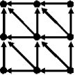
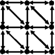
(a)	(b)
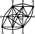
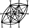
(c)	(d)

Figure 1: Upper pane: Interference structures for two types of $3\times 3$ 2-D channels: (a) ISI grid, (b) hexagonal Wyner cellular network. The arrows mark the direction of interference. Lower pane: The corresponding undirected graphical model representation of the channels in the upper pane: (c) ISI grid, (d) hexagonal Wyner cellular network. Full nodes represent (hidden) transmitted bits, while empty nodes correspond to the observations. Interaction couplings (compatibility function) $\psi_{ij}$ are denoted by a solid line connecting two full nodes, while the external field potential (evidence) $\phi_{i}$ is depicted by a solid line connecting a full node and an empty node. For clarity we use dotted edges in (d) to represent the extra edges added compared to the graph (c).

III Information rate

III-A Basic Definitions

The information rate, i.e. mutual information per symbol, between the channel’s input $\mathcal{X}$ and output $\mathcal{Y}$ is,

$$I(\mathcal{X};\mathcal{Y})=h(\mathcal{Y})-h(\mathcal{Y|X}),$$ (3)

where $h(\cdot)$ are (differential) entropy rates, where, by definition, the entropy rate $h(\mathcal{Q})$ of a stationary process ${\bf q}=\{q_{1},\ldots,q_{L}\}^{T}$ is given by $\lim_{L\rightarrow\infty}h({\bf q})/L$. Let us deal separately with the two terms in (3).

The second term, $h(\mathcal{Y|X})$, is given by $\lim_{N\rightarrow\infty}h({\bf y}|{\bf x})/N^{2}$, but since $h({\bf y}|{\bf x})=h({\bf v})$, and ${\bf v}$ is AWGN, it is straightforward to validate that $h(\mathcal{Y|X})=(\log{2\pi e\sigma^{2}})/2$.

In order to calculate $h(\mathcal{Y})$ we apply the Shannon-McMillan-Breiman theorem [13], which states that for a stationary and ergodic channel the entropy rate can be calculated by

$$-\frac{1}{N^{2}}\log p({\bf y})\stackrel{{\scriptstyle N\rightarrow\infty}}{{\longrightarrow}}h({\mathcal{Y}})~{}~{}\mbox{with probability}~{}~{}1,$$ (4)

where $p({\bf y})$ is the joint distribution of the channel’s output ${\bf y}$. Hence, in order to calculate the information rate one needs to calculate $p({\bf y})$ in the limit of large systems, as described in the next section.

III-B The Connection to Free Energy

Using Bayes’ law $p({\bf y})$ can be rewritten as

$$p({\bf y})=\sum_{{\bf x}}p({\bf y}|{\bf x})\Pr({\bf x})=\sum_{{\bf x}}p({\bf v})\Pr({\bf x}),$$ (5)

where $\sum_{{\bf x}}$ corresponds to a sum over all the possible values of the transmitted symbols ${\bf d}$. Hereinafter, for exposition purposes we consider the case of equiprobable i.i.d. binary-input alphabet, i.e., $d_{i}\in\pm 1$. Hence, using the distribution of ${\bf v}$, (5) can be rewritten as

$$p({\bf y})=\mathcal{Z}\cdot(2\mathcal{C})^{-N^{2}},$$ (6)

where $\mathcal{C}\triangleq(2\pi\sigma^{2})^{1/2}$, and

$$\mathcal{Z}\triangleq\sum_{{\bf x}}\exp{\bigg{(}-\frac{1}{2\sigma^{2}}||{\bf y}-{\bf S}{\bf x}||^{2}\bigg{)}},$$ (7)

is the partition function.

Inserting (6) into (4), the $I(\mathcal{X};\mathcal{Y})$ can be written as

$$\log{2}-1/2+\mathcal{F}\stackrel{{\scriptstyle N\rightarrow\infty}}{{\longrightarrow}}I({\mathcal{X}};{\mathcal{Y}})~{}~{}\mbox{with probability}~{}~{}1,$$ (8)

where

$$\mathcal{F}\triangleq-\frac{1}{N^{2}}\log(\mathcal{Z})$$ (9)

is recognized as the free energy per symbol [15, 12]. Hence, the problem of calculating the information rate boils down to estimating the free energy of an infinite system, as discussed in the next section. The information rate in (8) is termed the symmetric (a.k.a. uniform-input) information rate (SIR), due to the assumption regarding the uniformity of the input symbols. Similar analysis also holds for other stationary finite-state input distributions.

IV The Free Energy and the Cluster Variation Method

The free energy is a fundamental quantity in statistical mechanics which the physics literature has devoted a considerable effort in calculating. However, evaluating the free energy of infinitely large 2-D channels such as (1) is infeasible and, one must resort to approximate methods.

One of the classic approximation methods of free energies is the Kikuchi approximation, also known as the cluster variation method (CVM, [16]). The difficulty in exactly calculating the free energy results from the intractability of the probability distribution $p({\bf y})$. Hence, the CVM follows a variational principle: It defines the free energy as a functional of this probability distribution, $\mathcal{F}(p({\bf y}))$, replaces $p({\bf y})$ by a tractable trial belief vector $b({\bf y})$ , then minimizes $\mathcal{F}(b({\bf y}))$ w.r.t $b({\bf y})$, and considers the minimal value as its approximation to the free energy. Hence, our idea for estimating the information rate is to use the CVM over a large enough, yet finite, system, as the computed free energy per symbol is conjectured to converge to its exact value for infinite systems. This idea is empirically validated in section VI.

Recently, Yedidia et al. [16] have proved a correspondence between the stationary points of the CVM-based free energy and the fixed points of a message passing algorithm from the field of graphical models termed generalized belief propagation (GBP). GBP is an extension of the celebrated belief propagation algorithm (BP), that has been shown to provide better approximations than BP. Note, in passing, that Yedidia et al., have also shown that the fixed points of BP correspond to the stationary points of the Bethe free energy, which is a special case of the CVM, in the same way that BP is a special case of GBP. For an elaborate discussion of both CVM and GBP see [16]. In the following section we describe the channel from the perspective of graphical models, and shortly describe our application of the GBP algorithm.

V The connection to undirected graphical models

An undirected graphical model with pairwise potentials (a.k.a. pairwise Markov random fields), consists of a graph $G$ and potential (compatibility) functions $\psi_{ij}(\tilde{x_{i}},\tilde{x_{j}})$ and $\phi_{i}(\tilde{x_{i}})$ such that the probability of an assignment $\tilde{{\bf x}}$ is given by

$$\Pr(\tilde{{\bf x}})\propto\prod_{(i>j)}{\psi_{ij}(\tilde{x_{i}},\tilde{x_{j}})}\prod_{i}{\phi_{i}(\tilde{x_{i}})}.$$ (10)

The notation $(i>j)$ represents the set of all connected pairs $(\tilde{x_{i}},\tilde{x_{j}})$.

The joint posterior probability of the channel can be written as

$$\Pr({\bf x}|{\bf y})=\mathcal{Z}^{-1}\exp{\bigg{(}-\frac{1}{2\sigma^{2}}||{\bf y}-{\bf S}{\bf x}||^{2}\bigg{)}}.$$ (11)

Hence (11) defines the undirected graphical model

$$\Pr({\bf x}|{\bf y})\propto\prod_{(i>j)}{\psi_{ij}(x_{i},x_{j})}\prod_{i}{\phi_{i}(x_{i},h_{i})},$$ (12)

where

$$\psi_{ij}(x_{i},x_{j})=\exp\big{(}{-\frac{R_{ij}x_{i}x_{j}}{\sigma^{2}}}\big{)}$$ (13)

is a compatibility function representing the structure of the system and the potential

$$\phi_{i}(x_{i},y_{i})=\exp\big{(}{\frac{h_{i}x_{i}}{\sigma^{2}}}\big{)}$$ (14)

is the ’evidence’ or local likelihood, which describes the statistical dependency between the hidden variable $x_{i}$ and the observed variable $h_{i}$. The matrix ${\bf R}={\bf S}^{T}{\bf S}$ is the interference cross-correlation matrix and ${\bf h}={\bf S}^{T}{\bf y}$ is the output vector of a filter matched to the channel’s interference structure. The lower pane in Fig. 1 presents the resulting graphical models of the two channel examples considered in this work.

V-A Generalized Belief Propagation

The GBP algorithm is an extension of BP that has been shown to provide better approximations in many applications. The first step in applying GBP to a graph (10) is to define regions (clusters) of nodes which may intersect, and then pass messages between these regions in an analogous way to BP. Within each such region GBP performs exact inference, thus short cycles of nodes which are included in a region cause no problem.

Hence, a region that encompasses all nodes along the shortest cycles, might be a desired choice. Since the graphical models of our 2-D channel examples contain interactions between nearest neighbors and next nearest neighbors, as displayed in Fig. 1-(c,d), a natural choice of regions is a sliding $3\times 3$ square of nodes (e.g., see Fig 2). In all of our simulations the selected GBP regions were of size $3\times 3$. Surprisingly, the computations required for GBP are only slightly larger than the computations required for BP, and its complexity grows exponentially only with the size of the chosen regions.

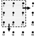
Figure 2: Covering a $4\times 4$ 2-D channel by $3\times 3$ regions used in GBP. Regions are defined by sliding a $3\times 3$ window along the channel. The result is four regions for this $4\times 4$ system:
$\{1,2,3,5,6,7,9,10,11\}$, $\{2,3,4,6,7,8,10,11,12\}$, $\{5,6,7,9,10,11,13,14,15\}$, $\{6,7,8,10,11,12,14,15,16\}$.

VI Simulation Results

VI-A Quality of the Free Energy Approximation

In order to evaluate the quality of our free energy approximation, we performed Monte-Carlo simulations of several channels. Fig. 3-(a) displays the root mean square (RMS) error per symbol, in percentage, between the approximated and exact free energies as a function of the channel’s size $N^{2}$ ($N=4,\ldots,9$, where a $9\times 9$ channel is the largest case for which exact computation was feasible.) The results were averaged over 500 realizations. As can be observed the difference between the approximated and exact free energies is minuscule (in the order of $10^{-4}\%$). These results were obtained for a specific channel, i.e., Wyner’s hexagonal cellular network, as depicted in Fig 1-(b), with $\alpha=0.5$ and signal to noise ratio (SNR) of $0$dB. Similar error performance was observed for all other channels, throughout the entire interference range and for a wide scope of SNR.

Fig. 3-(b) presents the CVM approximation of the free energy per symbol as a function of the channel’s size. The results were averaged over 500 channel realizations (for small channel size, $N\leq 9$, we used the same channel realizations as in Fig 3-(a).) It can be observed that the free energy per symbol converges with the size of the system, and that the differences among realizations become smaller. In principle, we could have simulated even larger systems, for which these differences would have been smaller. However, it seems that a $30\times 30$ system size suffices as an approximation of the exact free energy per symbol of infinite systems, thus can provide a proper estimate of the information rate.

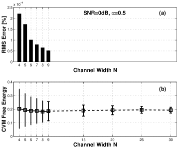
Figure 3: (a) Root mean square (RMS) error (in %) in computing the free energy per symbol, exactly and using the CVM, for $N\times N$ channels. The results were obtained using 500 realizations of Wyner’s hexagonal cellular networks (assuming a single user per cell), with $\alpha=0.5$ and SNR=$0$dB. (b) The corresponding CVM free energy per symbol as a function of $N$. For $N\leq 9$ we used the same realizations as in (a). For larger systems (dashed line) the exact free energy can not be calculated.

VI-B Information Rate Computation

The proposed GBP-based algorithm is used for estimating the SIR of two examples of dispersive 2-D channels: a 2-D ISI channel and an hexagonal Wyner cellular network. The results were obtained by averaging over $1000$ realizations of $30\times 30$ channels. The standard deviation of the results were small, thus are omitted from the figures.

2-D ISI Channel

We compute the SIR of a binary ISI channel with non-trivial ($\alpha=0.5$) interference structure as depicted in Fig. 1-(a). Fig. 4 presents the SIR, in terms of bit per symbol, computed using the GBP-based algorithm, as a function of SNR. Also drawn are the lower and upper bounds on the SIR, recently suggested by Chen and Siegel [10]. As can be seen the evaluated SIR agrees with these tight bounds.

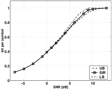
Figure 4: A 2-D ISI channel: SIR, in terms of bit per symbol, evaluated using GBP-based simulations (squares and a solid line), as a function of SNR. Also shown are upper (UB, dashed-dotted) and lower (LB, dashed) bounds on the SIR [10].

2-D Wyner Cellular Network

In a similar way, we computed the SIR of an hexagonal topology Wyner model [1], under binary signaling, with a single user within each cell (i.e. $K=1$ in Wyner’s notation). Fig. 5 displays the SIR calculated for the possible range of inter-cell interference scaling $\alpha$, for three SNR levels. For comparison we also present the Gaussian signaling capacity, as derived by Wyner. As may be expected for low SNR ($-10$dB) the SIR and Wyner’s capacity almost coincide. For the intermediate SNR level ($0$dB) Wyner’s capacity provides a tight upper bound on the SIR for $\alpha<0.5$. Note, in passing, that since the capacity of a binary channel is bounded between the SIR and Wyner’s Gaussian capacity, one can also infer the capacity in these low and intermediate SNR regimes. As for high SNR ($8$dB) the SIR saturates the $1$-bit bound, for almost all values of $\alpha$.

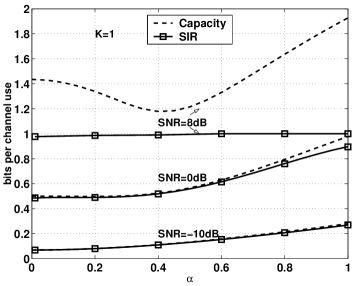
Figure 5: Hexagonal Wyner network: SIR (squares and solid line) and Gaussian signaling capacity (dashed), in bits per channel use, as a function of $\alpha$ for three SNR values: $-10$, $0$ and $8$ dB, and a single user within each cell ($K=1$).

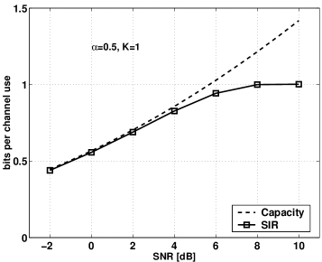
Figure 6: Hexagonal Wyner network: SIR (squares and solid line) and capacity (dashed), in bits per channel use, as a function of SNR for $\alpha=0.5$ and $K=1$.

In Fig. 6 we evaluated the SIR for a fixed $\alpha=0.5$ as a function of SNR. The SIR coincides with Wyner’s capacity for $\mbox{SNR}\lesssim 4$dB.

It should be emphasized that the analysis could have been performed, in a similar manner, for the case of several intra-cell users, i.e. $K>1$. This case corresponds to the case of $K=1$, where ($K+1$)-ary signaling from a binomial distribution, replaces the equiprobable binary signaling.

VII Discussion

In this paper we introduced a method for a simulation-based computation of the information rates of 2-D finite-state input channels with memory. Our method is established upon a connection between the information rate and the free energy, and on a graphical models based method of approximating this free energy. The quality of the approximation was compared to the exact free energy using small channels, and was found to exhibit practically accurate behavior, being consistent both as a function of the SNR and over the possible interference range. This behavior is then conjectured to hold for large, yet finite, systems, for which the information rate was estimated. In order to validate our method we compared the resulting information rate to formerly calculated bounds.

The physics and graphical models literature does not provide a rigorous explanation for this remarkable quality of approximation, as provided by the GBP-based CVM, thus research in this direction is currently underway.

References

- [1] A. D. Wyner, “Shannon-theoretic approach to a gaussian cellular multiple-access channel,” vol. 40, pp. 1713–1727, Nov. 1994.
- [2] W. Hirt, “Capacity and information rates of discrete-time channels with memory,” Ph.D. dissertation, Swiss Federal Inst. of Tech. (ETH), Zurich, Switzerland, 1998.
- [3] S. Shamai (Shitz), L. H. Ozarow, and A. D. Wyner, “Information rates for a discrete-time gaussian channel with intersymbol interference and stationary inputs,” vol. 37, no. 6, pp. 1527–1539, Nov. 1991.
- [4] J. Chen and P. H. Siegel, “Markov processes asymptotically achieve the capacity of finite state intersymbol interference channels,” To Appear.
- [5] A. Kavčić, “On the capacity of markov sources over noisy channels,” in Proc. IEEE Global Conference on Communications (GLOBECOM), San Antonio, Texas, USA, Nov. 2001, pp. 2997–3001.
- [6] S. Yang and A. Kavčić, “Markov sources achieve feedback capacity of finite-state machine channels,” in Proc. IEEE Int. Symp. Inform. Theory (ISIT), Lausanne, Switzerland, June 2002, p. 361.
- [7] S. Shamai (Shitz) and R. Laroia, “The intersymbol interference channel: lower bounds on capacity and precoding loss,” vol. 42, no. 5, pp. 1388–1404, Sept. 1998.
- [8] D. Arnold, H. A. Loeliger, P. O. Vontobel, A. Kavčić, and W. Zeng, “Simulation-based computation of information rates for channels with memory,” submitted for publication.
- [9] L. R. Bahl, J. Cocke, F. Jelinek, and J. Raviv, “Optimal decoding of linear codes for minimizing symbol error rate,” vol. 20, no. 3, pp. 284–287, Mar. 1974.
- [10] J. Chen and P. H. Siegel, “On the symmetric information rate of two-dimensional finite state ISI channels,” in Proc. IEEE Information Theory Workshop (ITW), Paris, France, Mar. 2003.
- [11] O. Shental, N. Shental, A. J. Weiss, and Y. Weiss, “Generalized belief propagation receiver for near-optimal detection of two-dimensional channels with memory,” in Proc. IEEE Information Theory Workshop (ITW), San Antonio, Texas, USA, Oct. 2004.
- [12] T. Tanaka, “A statistical-mechanics approach to large-system analysis of cdma multiuser detectors,” vol. 48, pp. 2888–2910, Nov. 2002.
- [13] T. M. Cover and J. A. Thomas, Elements of Information Theory. John Wiley and Sons, 1991.
- [14] B. G. Leroux, “Maximum-likelihood estimation for hidden markov models,” Stochastic Processes and their Applications, vol. 40, pp. 127–143, 1992.
- [15] M. Mézard, G. Parisi, and M. A. Virasoro, Spin Glass Theory and Beyond. Singapore: World Scientific Lecture Notes in Physics Vol. 9, 1987.
- [16] J. S. Yedidia, W. T. Freeman, and Y. Weiss, “Constructing free energy approximations and generalized belief propagation algorithm,” Mitsubishi Electric Laboratories, Cambridge, MA, Tech. Rep. TR-2004-40, May 2004. [Online]. Available: http://www.merl.com