Analysis of Second-order Statistics Based Semi-blind Channel Estimation in CDMA Channels

2005 Conference on Information Sciences and Systems, The Johns Hopkins University, March 16–18, 2005

Analysis of Second-order Statistics Based Semi-blind Channel Estimation in CDMA Channels
Husheng Li and H. Vincent Poor Department of Electrical Engineering
Princeton University
Princeton, NJ 08544
e-mail: {hushengl,poor}@princeton.edu

Abstract — The performance of second order statistics (SOS) based semi-blind channel estimation in long-code DS-CDMA systems is analyzed. The covariance matrix of SOS estimates is obtained in the large system limit, and is used to analyze the large-sample performance of two SOS based semi-blind channel estimation algorithms. A notion of blind estimation efficiency is also defined and is examined via simulation results.

I. Introduction

In practical wireless communication systems, the transmitted signals usually experience fading, which either attenuates the received power or causes dispersion. Usually, the channel state information is unknown to both the transmitter and the receiver in many practical applications, thus necessitating channel estimation at the frontend of the coherent receiver. In this paper, we focus on the long-code direct-sequence code division multiple-access (DS-CDMA) systems and frequency-selective fading channels.

A variety of channel estimation algorithms have been derived, based primarily on one of two aspects of random observations, namely, the distribution and the moments. When the distribution of the received signal conditioned on the channel state information is known, the maximum likelihood (ML) criterion can be applied to yield asymptotically optimal performance. Such ML channel estimation algorithms [3] are suitable for training-symbol-based systems, in which a fraction of the transmitted symbols is known to both the transmitter and receiver. However, the channel state information hidden in the information symbols is ignored, thus decreasing the spectral efficiency.

When only the information symbols are available (usually called blind channel estimation), the moment based channel estimation algorithms require substantially less computational cost than other methods, thus being feasible for practical applications. Thus, over the past two decades, a large number of blind channel estimation algorithms [1][7][11][13] have been developed using moment estimation, particularly the second order statistics (SOS). Typically, based on SOS estimation, the subspace method [1] and moment matching  [11] can be applied. The subspace technique is suitable only for stationary channels, e.g. short-code CDMA systems, since it requires the signal subspace to be time-invariant. However, in many practical CDMA systems, long codes are employed, thus making the overall channel non-stationary. Therefore, only the moment matching technique can be applied directly to long-code CDMA systems. When training symbols are available, both the training and information symbols can be used jointly to yield better estimates (usually called semi-blind channel estimation).

In this paper, we adopt the moment-matching-based algorithm of [11] for estimating the SOS of channel coefficients of each user. The following two SOS based semi-blind channel estimation algorithms are considered.

• Moment-matching-based estimation. The asymptotically optimal moment based estimator [8] is applied to the first order moment, estimated from the training symbols, and the SOS, estimated from the information symbols, thus resulting in moment-matching-based semi-blind channel estimation under some assumptions.

• Subspace-based estimation. The subspace spanned by the channel coefficient vector is obtained from the eigenstructure of SOS estimation. The channel estimates are obtained by projecting the training symbols onto the subspace followed by linear combining. It should be noted that the subspace here is different from that mentioned above, which is spanned by the signal.

The remainder of this paper is organized as follows. A discrete model of the frequency selective fading channels is explained in Section II. The performance of SOS estimation and semi-blind channel estimation is analyzed in Section III and Section IV, respectively. Simulation results and conclusions are given in Section V and Section VI, respectively. The details can be found in the journal version of this paper [6].

II. System Model

We consider a synchronous uplink DS-CDMA system operating over frequency selective fading channels of order $P$ (i.e, $P$ is the delay spread in chip intervals). Let $K$ denote the number of active users, $N$ the spreading gain and $\beta\triangleq\frac{K}{N}$ the system load. We model the frequency selective fading channels with discrete finite-impulse-response (FIR) filters. The $z$-transform of the channel response of user $k$ is thus given by

$$h_{k}(z)=\sum_{p=0}^{P-1}g_{k}(p)z^{p},$$ (1)

where $\{g_{k}(p)\}_{p=0,...,P-1}$ are the corresponding independent and identically distributed (i.i.d.) (with respect to both $k$ and $p$) channel coefficients with variance $\frac{1}{P}$. We adopt the block fading model, in which the channel coefficients, namely $\{{g}_{k}(p)\}$, remain unchanged during a coherent block, and we denote the coherence time by $M$, measured in channel symbol periods.

With the assumption $P\ll N$, we can ignore the effects of intersymbol interference (ISI). Thus, the chip matched filter output at the $l$-th chip period in the $m$-th symbol period can be written as

$$r(mN+l)=\sum_{k=1}^{K}x_{k}(m)h_{k}^{(m)}(l)+n(mN+l),$$ (2)

where $\{x_{k}(m)\}$ denotes the complex channel symbols, which are mutually independent with respect to $k$ and $m$. We assume that $x_{k}(m)$ is a complex random variable satisfying $E\left\{\left|x_{k}(m)\right|^{2}\right\}=1$ and $E\left\{x_{k}^{2}(m)\right\}=0$, which hold, for example, for quadratic phase shift keying (QPSK) modulation. $\{n(mN+l)\}$ is additive white complex Gaussian noise, which satisfies $E\{|n(mN+l)|^{2}\}=\sigma_{n}^{2}$ . $\{h_{k}^{(m)}(l)\}$ denote the convolution of the spreading code and the channel coefficients:

$$h_{k}^{(m)}(l)=s_{k}^{(m)}(l)\star g_{k}(l),$$ (3)

where $s_{k}^{(m)}(l)$ is the $l$-th chip of the original random spreading codes of user $k$ in symbol period $m$, which takes values $\frac{1}{\sqrt{N}}$ and $-\frac{1}{\sqrt{N}}$ equiprobably and independently with respect to $k$, $m$ and $l$.

When the channel coefficients are unknown to the receiver, channel estimation is necessary for coherent reception. For simplicity, we assume that $M_{t}$ training symbols, which are known to both transmitter and receiver, are transmitted at the beginning of each coherent block, and the proportion of training symbols is denoted by $\alpha=\frac{M_{t}}{M}$.

III. Performance of SOS Estimation

When discussing SOS estimation in this section, for notational simplicity, we assume that all $M$ channel symbols during the coherent block are unknown to the receiver. When analyzing the performance of semi-blind channel estimation, we can simply replace $M$ with $M-M_{t}$ in the conclusions for SOS estimation. It should be noted that our analysis on the performance of SOS estimation is based on the large system limit, namely $K,N\rightarrow\infty$ while keeping $\beta$ and $P$ constant.

A SOS Estimation Algorithm

We adopt the algorithm proposed in  [11] to estimate the channel coefficients in long-code CDMA systems. On defining $\mathbf{r}(m)=\left(r(mN+P),...,r((m+1)N)\right)^{T}$ as the signal unaffected by ISI during the symbol period $m$, we can rewrite (2) in vector form, which is given by

$$\mathbf{r}(m)=\sum_{k=1}^{K}C_{k}^{(m)}\mathbf{g}_{k}x_{k}(m)+\mathbf{n}(m),$$ (4)

where $\mathbf{g}_{k}=\left(g_{k}(0),...,g_{k}(P-1)\right)^{T}$, $\mathbf{n}_{k}(m)=\left(n(mN+P),...,n((m+1)N)\right)^{T}$ and $C_{k}^{(m)}$ is the truncated Sylvester matrix, which is given by

$$C_{k}^{(m)}=\left(\begin{array}[]{llll}s_{k}^{(m)}(P)&s_{k}^{(m)}(P-1)&\ldots&s_{k}^{(m)}(1)\\ s_{k}^{(m)}(P+1)&s_{k}^{(m)}(P)&\ldots&s_{k}^{(m)}(2)\\ \vdots&\vdots&\ldots&\vdots\\ s_{k}^{(m)}(N)&s_{k}^{(m)}(N-1)&\ldots&s_{k}^{(m)}(N-P+1)\\ \end{array}\right).$$ (9)

We define a cost function for moment matching, which is given by

$$J=\left\|\sum_{m=1}^{M}\left(E\left\{\mathbf{R}_{r}(m)\right\}-\mathbf{R}_{r}(m)\right)\right\|_{F},$$ (10)

where $\mathbf{R}_{r}(m)=\mathbf{r}(m)\mathbf{r}(m)^{H}$ and $\|\cdot\|_{F}$ denotes the Frobenius norm. The optimal SOS is obtained by minimizing the cost function $J$,

$$\hat{\mathbf{d}}=\arg\min_{d}J,$$

where $\mathbf{d}=\left(\mathbf{d}_{1}^{H},...,\mathbf{d}_{k}^{H}\right)^{H}$, $\mathbf{d}_{k}=\mbox{vec}\left(\mathbf{g}_{k}\mathbf{g}_{k}^{H}\right)$ and $\mbox{vec}(X)$ denotes a vector formed by stacking the columns of matrix $X$ into one column vector. An explicit expression for $\hat{\mathbf{d}}$ is obtained in  [11], which is given by

$$\hat{\mathbf{d}}=\mathbf{T}^{-1}\mathbf{y},$$ (11)

where

$$\mathbf{T}_{P^{2}K\times P^{2}K}=\frac{1}{M}\sum_{m=1}^{M}Q^{T}(m)Q(m),$$

$$\mathbf{y}_{P^{2}K\times 1}=\frac{1}{M}\sum_{m=1}^{M}Q^{T}(m)\mbox{vec}\left(\mathbf{r}(m)\mathbf{r}^{H}(m)\right)-\sigma_{n}^{2}Q^{T}(m)\mbox{vec}(\mathbf{I}),$$

$$Q(m)_{(N-P+1)^{2}\times P^{2}K}=\left(Q_{1}(m),Q_{2}(m),...,Q_{K}(m)\right),$$

and

$$Q_{k}(m)_{(N-P+1)^{2}\times P^{2}}=C_{k}^{(m)}\otimes C_{k}^{(m)},$$

where $\otimes$ denotes the Kronecker product. In practical implementations, $\hat{\mathbf{d}}$ can be obtained by solving (11) iteratively.

B Identifiability and Consistency

On analyzing the elements of $\mathbf{T}$, we obtain the following lemma.

Lemma III.1

$\mathbf{T}$ converges elementwise to $\mathbf{I}$ almost surely as $M\rightarrow\infty$ and $N\rightarrow\infty$.

In  [11], it is shown that the channel is identifiable and that SOS based channel estimation is consistent if $\mathbf{T}$ is nonsingular. We cannot draw the conclusion that $\mathbf{T}$ is nonsingular as $M\rightarrow\infty$ and $N\rightarrow\infty$ merely from Lemma III.1, since the corresponding convergence is elementwise and not in norm. However, we can show the following proposition, which states a sufficient condition for the non-singularity of $E\{\mathbf{T}\}$.

Proposition III.2

Suppose $K$ and $N$ are such that $KP<N-P+1$. Then $E\{\mathbf{T}\}$ is nonsingular and $\left\|E\{\mathbf{T}\}^{-1}-\mathbf{I}\right\|_{1}$ is finite.

As $K$ and $N$ become sufficiently large, the condition that $KP<N-P+1$ is equivalent to $\beta<\frac{1}{P}$. Since $\mathbf{T}$ converges to $E\{\mathbf{T}\}$ almost surely as $M\rightarrow\infty$, $\mathbf{T}$ is nonsingular with large probability when $M$ is sufficiently large. Since $\left\|E\{\mathbf{T}\}^{-1}-\mathbf{I}\right\|_{1}$ is finite as $K,N\rightarrow\infty$, most of the elements of $E\{\mathbf{T}\}^{-1}$ converge to the corresponding elements of $\mathbf{I}$. Thus it is reasonable to approximate $\mathbf{T}^{-1}$ with $\mathbf{I}$ when $K$ and $N$ are sufficiently large. For the case $\beta>\frac{1}{P}$, numerical simulation indicates that the non-singularity of $\mathbf{T}$ still typically holds. Thus, in the following analysis of SOS estimation error, we assume that $\mathbf{T}=\mathbf{I}$, which will be validated later by simulation results.

C SOS Estimation Error

The SOS estimation error $\delta\mathbf{d}_{k}\triangleq\hat{\mathbf{d}}_{k}-\mathbf{d}_{k}$ is due to the multiple-access interference (MAI) and noise. The following proposition gives an explicit expression for the covariance matrix of $\delta\mathbf{d}_{k}$, where the assumptions can be shown to hold in elementwise convergence as $K,N\rightarrow\infty$.

Proposition III.3

Assume

$$\sum_{i,j=1,i\neq j}^{K}Q_{ij}(m)\mathbf{d}_{ij}\mathbf{d}_{ij}^{H}Q_{ij}^{T}(m)=\beta^{2}\mathbf{I}_{(N-P+1)^{2}\times(N-P+1)^{2}}.$$

$$\sum_{k=2}^{K}\left(C_{k}^{(m)}\otimes\mathbf{n}(m)\right)\mathbf{g}^{*}_{k}\mathbf{g}^{T}_{k}\left(C_{k}^{(m)}\otimes\mathbf{n}(m)\right)^{H}=\beta\sigma_{n}^{2}$$

and

$$\sum_{k=1}^{K}\left(\mathbf{n}^{*}(m)\otimes C_{k}^{(m)}\right)\mathbf{g}_{k}\mathbf{g}^{H}_{k}\left(\mathbf{n}^{*}(m)\otimes C_{k}^{(m)}\right)^{H}=\beta\sigma_{n}^{2}.$$

Then we have, for $k=1,...,K$, as $K,N\rightarrow\infty$,

$$\Sigma^{k}_{\delta\mathbf{d}} \triangleq ME\left\{\delta\mathbf{d}_{k}\delta\mathbf{d}_{k}^{H}\right\}$$ (12)

$$\rightarrow \left(2\beta\sigma_{n}^{2}+(\sigma_{n}^{2})^{2}+\beta^{2}+\frac{2\beta}{P}\right)\mathbf{I}_{P^{2}\times P^{2}}+\sigma_{n}^{2}{\bf{\Omega}}_{k}.$$

where

$$\left(\bf{\Omega}_{k}\right)_{ij}=\left\{\begin{array}[]{llll}\left|\left(\mathbf{g}_{k}\right)_{\left\lceil\frac{i}{P}\right\rceil}\right|^{2}+\left|\left(\mathbf{g}_{k}\right)_{\mbox{mod}(i,P)}\right|^{2},\qquad\mbox{if }i=j\\ \left(\mathbf{g}_{k}\right)^{*}_{\left\lceil\frac{i}{P}\right\rceil}\left(\mathbf{g}_{k}\right)_{\left\lceil\frac{j}{P}\right\rceil},\qquad\mbox{otherwise, if }\mbox{mod}(i,P)=\mbox{mod}(j,P)\\ \left(\mathbf{g}_{k}\right)_{\mbox{mod}(i,P)}\left(\mathbf{g}_{k}\right)^{*}_{\mbox{mod}(j,P)},\qquad\mbox{otherwise, if }\left\lceil\frac{i}{P}\right\rceil=\left\lceil\frac{j}{P}\right\rceil\\ 0,\qquad\mbox{otherwise}\end{array}\right..$$ (17)

An interesting observation on (12) is that the SOS estimation errors are mutually correlated and the covariance matrix is dependent on the realization of channel coefficients. However, when $\beta$ is moderate or large, the correlation is weak, compared with the error variance. We can apply the asymptotic results in (12) to finite systems as approximations.

For the average SOS estimation variance of all users, we have

$$\sigma_{d}^{2} \triangleq \frac{1}{KP^{2}}\sum_{k=1}^{K}\Sigma_{\delta d}^{k}$$

$$\rightarrow 2\beta\sigma_{n}^{2}+\left(\sigma_{n}^{2}\right)^{2}+\beta^{2}+\frac{2(\beta+\sigma_{n}^{2})}{P},$$

from which we can see that the performance of SOS estimation is determined by the system load and noise variance.

It should be noted that it is not sufficient to obtain $E\left\{\delta\mathbf{d}_{k}\delta\mathbf{d}_{k}^{H}\right\}$ for the performance analysis of semi-blind channel estimation, since the channel coefficients are complex. $E\left\{\delta\mathbf{d}_{k}\delta\mathbf{d}_{k}^{T}\right\}$ is also necessary for the analysis in the next section. However, it is easy to check that, for all $1\leq i,j\leq P^{2}$,

$$\left(E\left\{\delta\mathbf{d}_{k}\delta\mathbf{d}^{T}_{k}\right\}\right)_{i,j}=\frac{1}{M}\left(\Sigma^{k}_{\delta\mathbf{d}}\right)_{i,\left(\small\mbox{mod}(j,P)-1\right)P+\left\lceil\frac{j}{P}\right\rceil}.$$

Then, it is further easy to check that $\left(E\left\{\delta\mathbf{d}_{k}\delta\mathbf{d}^{T}_{k}\right\}\right)_{i,i}=0$, $i=1,...,P^{2}$, except for $\left\lceil\frac{i}{P}\right\rceil=\mbox{mod}(i,P)$ which means that $\left(\mathbf{d}_{k}\right)_{i}$ are the diagonal elements of $\mathbf{g}\mathbf{g}^{H}$, and thus are real. Therefore, we can conclude that the real and imaginary parts of the SOS estimation error are uncorrelated and have identical variances.

IV. Performance of Semi-blind Channel Estimation

In this section, we consider two approaches to semi-blind channel estimation, namely moment-matching-based and subspace-based algorithms. In semi-blind channel estimation, $M_{t}$ training symbols are available (thus, the number of information symbols is $M-M_{t}$) and the corresponding received training signal, which is represented by a $NM_{t}$-vector, is given by

$$\mathbf{r}_{t}=\sum_{k=1}^{K}C_{t}(k)\mathbf{g}_{k}+\mathbf{n}_{t},$$ (18)

where, similarly to (4), $C_{t}(k)$ is the Sylvester matrix constructed by

$$\tilde{\mathbf{s}}_{k}=\left(\left(\mathbf{s}_{k}^{(1)}x_{k}(1)\right)^{H},...,\left(\mathbf{s}_{k}^{(M_{t})}x_{k}(M_{t})\right)^{H}\right)^{H}.$$

By multiplying $\frac{1}{M_{t}}C_{t}^{T}(k)$ on both sides of (18), the MAI for user $k$ can be completely cancelled, as $M_{t}\rightarrow\infty$ since $\frac{1}{M_{t}}C_{t}^{T}(k)C_{t}(k)\rightarrow\mathbf{I}$. Therefore, a sufficient statistic for $\mathbf{g}_{k}$ is given by $\bar{\mathbf{g}}_{k}\triangleq\frac{1}{M_{t}}C_{t}^{T}(k)\mathbf{r}_{t}$. Thus, the equivalent training signal for user $k$ is given by

$$\bar{\mathbf{g}}_{k}=\mathbf{g}_{k}+\tilde{\mathbf{n}}_{k},$$ (19)

where $\tilde{\mathbf{n}}_{k}=\frac{1}{M_{t}}C_{t}^{T}(k)\mathbf{n}_{t}$ is additive white complex Gaussian noise with variance $\frac{\sigma_{n}^{2}}{M_{t}}$. As $M_{t}\rightarrow\infty$, $\left(\tilde{\mathbf{n}}_{k}\right)_{l}$ become mutually independent with respect to $k$ and $l$.

Since both $\left\{\bar{\mathbf{g}}_{k}\right\}$ and $\left\{{\mathbf{d}}_{k}\right\}$ across different users are weakly correlated when $M$ is sufficiently large , we can carry out the channel estimation for each user separately, thereby reducing considerably the computational complexity at cost of marginal performance loss. For notational simplicity, we drop the subscripts of user index throughout this section. The elements in $\mathbf{g}$ and $\mathbf{d}$ are denoted by $g_{p}$, $p=1,...,P$, and $d_{p}$, $p=1,...,P^{2}$, respectively.

A Moment Matching

A.1 Moment-matching-based estimator

For applying the asymptotically optimal estimator in  [8] and the corresponding analysis, it is necessary to discuss the moment based channel estimation in $\mathbb{R}$. For any complex vector $\mathbf{v}$, we denote the corresponding real vector by $\mathsf{v}\triangleq\left(\Re\left(\mathbf{v}\right)^{T},\Im\left(\mathbf{v}\right)^{T}\right)^{T}$, where $\Re\left(\mathbf{v}\right)$ and $\Im\left(\mathbf{v}\right)$ represent the real and imaginary parts of $\mathbf{v}$.

It should be noted that there are only $\frac{P(P+1)}{2}$ free variables in $\hat{\mathbf{d}}$ and $P^{2}$ free variables in $\hat{\mathsf{d}}$ (note that there are $P$ real elements in $\hat{\mathbf{d}}$, corresponding to the diagonal elements in $\mathbf{g}\mathbf{g}^{T}$) since $\hat{\mathbf{d}}$ is the vectorization of a Hermite matrix. We denote the real vector of these free variables by $\hat{\mathsf{d}}_{f}$, where the subscript f means free.

On defining the observation vector $\hat{\mathsf{z}}\triangleq\left(\bar{\mathsf{g}}^{T},\hat{\mathsf{d}}_{f}^{T}\right)^{T}$, $\mathsf{z}\triangleq\left(\mathsf{g}^{T},\mathsf{d}_{f}^{T}\right)^{T}$ and $\delta\mathsf{z}\triangleq\hat{\mathsf{z}}-\mathsf{z}$, the asymptotically optimal estimator using estimates of the first and second moments [8] is obtained by minimizing a cost function, which is given by

$$J_{{opt}}\left(\hat{\mathbf{g}}\right)=\left(\tilde{\mathsf{z}}\left(\hat{\mathbf{g}}\right)-\hat{\mathsf{z}}\right)^{T}\left(\Sigma_{\delta{\mathsf{z}}}\right)^{-1}\left(\tilde{\mathsf{z}}\left(\hat{\mathbf{g}}\right)-\hat{\mathsf{z}}\right),$$ (20)

where $\Sigma_{\delta{\mathsf{z}}}\triangleq E\left\{\delta{\mathsf{z}}\delta{\mathsf{z}}^{T}\right\}$ and the function $\tilde{\mathsf{z}}$ maps $\mathbf{g}$ to $\mathsf{z}$.

It is easy to check that

$$\Sigma_{\delta\mathsf{z}}=\left(\begin{array}[]{ll}\frac{\sigma_{n}^{2}}{2M_{t}}\mathbf{I}_{2P\times 2P}&0\\ 0&\frac{1}{M-M_{t}}\Sigma_{\delta\mathsf{d}_{f}}\end{array}\right),$$

where the covariance matrix $\Sigma_{\delta\mathsf{d}_{f}}$ can be obtained from Prop. III.3.

However, due to the conclusion of Prop. III.3, $\Sigma_{\delta\mathsf{d}_{f}}$ is dependent on the realization of $\mathbf{g}$, thus being unknown to the estimator. Therefore, the optimal estimator is infeasible for practical applications. Since the cross correlation of different elements in $\mathbf{d}_{f}$ is small for moderate or large $\beta$, we can assume that $\Sigma_{\delta\mathsf{d}_{f}}=\sigma_{d}^{2}\mathbf{I}$, thus resulting in the cost function given by

$$J\left(\hat{\mathbf{g}}\right)=w\left\|\mbox{vec}\left(\hat{\mathbf{g}}\hat{\mathbf{g}}^{H}\right)-\hat{\mathbf{d}}\right\|^{2}+(1-w)\left\|\hat{\mathbf{g}}-\bar{\mathbf{g}}\right\|^{2},$$ (21)

where the weighting factor $w=\frac{(1-\alpha)\sigma_{n}^{2}}{(1-\alpha)\sigma_{n}^{2}+\alpha\sigma_{d}^{2}}$. Since minimizing (21) is equivalent to obtaining $\hat{\mathbf{g}}$, which optimally matches the first and second moment estimates in $\hat{\mathsf{z}}$, we call it moment matching based channel estimation.

A.2 Performance analysis

Practically, the cost function (21) can be minimized with iterative optimization methods. For theoretical analysis, the optimal $\mathbf{g}$ can also be obtained by taking derivatives of the cost function (21) with respect to $\hat{\mathsf{g}}$, resulting in $2P$ equations denoted by $F_{i}=0$, $i=1,...,2P$. These equations determine a mapping ${\bf{\Psi}}$ from the observation $\hat{\mathsf{z}}$ to $\hat{\mathsf{g}}$ in a neighborhood of $\mathsf{z}$. Thus, by applying the implicit function theorem [9], we can obtain the Jacobian matrix of ${\bf{\Psi}}$ at $\mathsf{z}$, which is given by

$$\frac{\partial{\bf{\Psi}}}{\partial\hat{\mathsf{z}}}\bigg{|}_{\hat{\mathsf{z}}=\mathsf{z}}=-\left(\frac{\partial\mathbf{F}}{\partial\hat{\mathsf{g}}}\right)^{-1}\bigg{|}_{\hat{\mathsf{g}}=\mathsf{g}}\frac{\partial\mathbf{F}}{\partial\hat{\mathsf{z}}}\bigg{|}_{\hat{\mathsf{z}}=\mathsf{z}},$$ (22)

where $\mathbf{F}\triangleq\left(F_{1},...,F_{2P}\right)^{T}$, provided that $\frac{\partial\mathbf{F}}{\partial\hat{\mathsf{g}}}$ is non-singular.

Therefore, for the channel estimation error $\delta\mathsf{g}=\hat{\mathsf{g}}-\mathsf{g}$, we have the following proposition, whose proof is essentially the same as that of Theorem 3.16 in  [8] and is omitted in this paper.

Proposition IV.1

In moment-matching-based semi-blind channel estimation, if $\sqrt{M}\delta\mathsf{z}$ converges weakly to a random vector with zero mean and a covariance matrix $\Sigma_{\delta\mathsf{z}}$ as $M\rightarrow\infty$, then $M\delta\mathsf{g}$ converges weakly to a random vector with zero mean and covariance matrix given by

$$\Sigma_{\delta\mathsf{g}}=\left(\frac{\partial{\bf{\Psi}}}{\partial\hat{\mathsf{z}}}\Sigma_{\delta\mathsf{z}}\left(\frac{\partial{\bf{\Psi}}}{\partial\hat{\mathsf{z}}}\right)^{T}\right)\bigg{|}_{\hat{\mathsf{z}}=\mathsf{z}},$$ (23)

provided that the Jacobian matrix $\frac{\partial{\bf{\Psi}}}{\partial\hat{\mathsf{z}}}\big{|}_{\hat{\mathsf{z}}=\mathsf{z}}$ is nonsingular.

A.3 Performance bound

Using Lemma 3.1 in [8], the asymptotic performance of SOS based blind channel estimation can be lower bounded by that of the asymptotically optimal estimator, which is given by

$$\Sigma_{\delta\mathsf{g}}\geq\left(\left(\frac{\partial\hat{\mathsf{z}}}{\partial\hat{\mathsf{g}}}\right)^{T}\Sigma_{\delta\mathsf{z}}^{-1}\frac{\partial\hat{\mathsf{z}}}{\partial\hat{\mathsf{g}}}\right)^{-1}\bigg{|}_{\hat{\mathsf{g}}=\mathsf{g}},$$ (24)

where

$$\frac{\partial\hat{\mathsf{z}}}{\partial\hat{\mathsf{g}}}\bigg{|}_{\hat{\mathsf{g}}=\mathsf{g}}=\left(\begin{array}[]{ll}\mathbf{I}_{2P\times 2P}\\ \frac{\partial\hat{\mathsf{d}}_{f}}{\partial\hat{\mathsf{g}}}\bigg{|}_{\hat{\mathsf{g}}=\mathsf{g}}\end{array}\right),$$ (27)

B Subspace-based Approach

B.1 Subspace-based estimator

Another methodology for semi-blind channel estimation is to make use of the subspace estimated from the SOS estimates. In this section, we adopt a simple subspace algorithm, which can be carried out in the following three steps:

1. The one-dimensional subspace spanned by $\mathbf{g}$ is obtained from the unit eigenvector $\mathbf{u}$ of matrix $\mbox{vec}^{-1}\left(\hat{\mathbf{d}}\right)$ corresponding to its largest eigenvalue.

2. The channel estimate from the training symbols, namely $\bar{\mathbf{g}}$, is projected onto the subspace, thus decreasing the noise power and obtaining a tentative channel estimate, which is given by

   $$\tilde{\mathbf{g}}={\mathbf{u}}^{H}\bar{\mathbf{g}}{\mathbf{u}}.$$ (28)

3. The final channel estimate is obtained by combining $\bar{\mathbf{g}}$ and $\tilde{\mathbf{g}}$ linearly:

   $$\hat{\mathbf{g}}=\omega\tilde{\mathbf{g}}+(1-\omega)\bar{\mathbf{g}},$$

   where $\omega$ is a weighting factor, which will be optimized later.

This algorithm can also be regarded as tackling the phase ambiguity incurred by SOS based blind channel estimation by making use of the training symbols.

B.2 Perturbation on signal subspace

On denoting the acute angle between the subspace spanned by $\mathbf{g}$ and the unit eigenvector ${\mathbf{u}}$ by $\theta=\arccos\left(\frac{\left|\mathbf{g}^{H}{\mathbf{u}}\right|}{\left\|\mathbf{g}\right\|}\right)$, we can obtain an explicit asymptotic expression for $E\left\{\sin^{2}\theta\right\}$, which is given in the following Proposition.

Proposition IV.2

As $K,N,M\rightarrow\infty$,

$$\sigma_{\theta}^{2} \triangleq ME\left\{\sin^{2}\theta\right\}$$ (29)

$$\rightarrow \frac{(P-1)\left(\left(2\beta+\|\mathbf{g}\|^{2}\right)\sigma_{n}^{2}+\left(\sigma_{n}^{2}\right)^{2}+\beta^{2}+\frac{2\beta}{P}\right)}{\|\mathbf{g}\|^{4}}.$$

C Performance of channel estimation

On defining $\delta{\mathbf{u}}\triangleq\frac{-\mathbf{g}+{\mathbf{u}}^{H}\mathbf{g}{\mathbf{u}}}{\|\mathbf{g}\|}$, (28) can be rewritten as

$$\tilde{\mathbf{g}}=\frac{\|\mathbf{g}\|^{2}}{\left|\mathbf{u}^{H}\mathbf{g}\right|^{2}}\left(\frac{\mathbf{g}}{\|\mathbf{g}\|}+\delta{\mathbf{u}}\right)^{H}\left(\mathbf{g}+\tilde{\mathbf{n}}\right)\left(\frac{\mathbf{g}}{\|\mathbf{g}\|}+\delta{\mathbf{u}}\right),$$

where $\tilde{\mathbf{n}}$ is defined in (19). It is easy to check that $\delta{\mathbf{u}}^{H}\delta{\mathbf{u}}\approx\sin^{2}\theta$, which becomes tight as $\theta\rightarrow 0$. We assume that the different elements in $\delta{\mathbf{u}}$ are mutually independent, and the real and imaginary parts of each element are also mutually independent with identical variances. These assumptions can be validated by simulation.

By ignoring the higher order terms and applying $\left|\mathbf{u}^{H}\mathbf{g}\right|^{2}\rightarrow\|\mathbf{g}\|^{2}$, we can obtain

$$\sigma_{g}^{2} \triangleq \frac{ME\left\{\delta\mathbf{g}^{H}\delta\mathbf{g}\right\}}{P}$$ (30)

$$= \frac{\omega^{2}\|\mathbf{g}\|^{2}\left(1+\frac{1}{P}\right)\sigma_{\theta}^{2}}{(1-\alpha)P}+\frac{(1-\omega)^{2}(P-1)\sigma_{n}^{2}}{P\alpha}+\frac{\sigma_{n}^{2}}{P\alpha},$$

where the optimal $\omega$ is given by

$$\omega_{opt}=\frac{\frac{(P-1)\sigma_{n}^{2}}{\alpha}}{\frac{\|\mathbf{g}\|^{2}\left(1+\frac{1}{P}\right)\sigma_{\theta}^{2}}{1-\alpha}+\frac{(P-1)\sigma_{n}^{2}}{\alpha}}.$$ (31)

When $\omega=0$, $\sigma_{g}^{2}=\frac{\sigma_{n}^{2}}{\alpha}$, which equals the performance of training-symbol-based estimation. Thus, the subspace-based channel estimation with optimal $\omega$ surely attains better performance than training symbol based estimation. When the subspace estimation is perfect and $\omega=1$, $\sigma_{g}^{2}=\frac{\sigma_{n}^{2}}{\alpha P}$, which means that noise level is lowered by a factor of $\frac{1}{P}$. Therefore, the last term in (30) is the performance with perfect SOS estimation and the first term in (30) represent the penalty incurred by imperfect SOS estimation.

V. Simulation results

A Moment-matching-based Channel Estimation

We define the blind estimation efficiency as

$$\eta\triangleq\frac{\frac{\sigma_{n}^{2}}{\sigma_{g}^{2}}-\alpha}{1-\alpha}.$$ (32)

Intuitively, $\eta$ quantifies how many training symbols each information symbol is equivalent to for the purpose of semi-blind channel estimation. Figure 1 shows the efficiency $\eta$ obtained from Prop. IV.1 versus $\beta$ and $\sigma_{n}^{2}$ when $P=3$ and $\alpha=0.2$. We observe that $\eta$ decreases monotonically with $\beta$ since larger $\beta$ implies more MAI for SOS estimation. An interesting observation is that the efficiency is small for both high and low noise levels and achieves a maximum (around 0.3) for moderate noise power (around $\sigma_{n}^{2}=1$). An intuitive explanation is that, when $\sigma_{n}^{2}$ is large, the SOS estimation performance is poor since the SOS error variance contains a term proportional to $\left(\sigma_{n}^{2}\right)^{2}$; when $\sigma_{n}^{2}$ is small, the SOS estimation error is dominated by the MAI, thus achieving much lower efficiency than training-symbol-based estimation.

Figure 2 shows the efficiency versus $P$ and $\alpha$ when $\sigma_{n}^{2}=0.5$ and $\beta=0.5$. An important observation from this figure is that, for large $\alpha$ and $P$, the efficiency $\eta<0$, which means that it is harmful to incorporate the information symbols into the channel estimation. This arises from the suboptimality of the channel estimator in (21) since the exact covariance matrix of the SOS estimation error is unknown and the estimated weighting factor $w$ is also suboptimal. Thus, the unreliable SOS estimation may have negative impact on the reliable estimation from the training symbols, when $\alpha$ is large. When $\alpha$ is small, the efficiency achieves its maximum for small $P$; however, the efficiency does not change much with respect to $P$.

From the simulation results of Fig. 1 and Fig. 2, we can draw a conclusion that moment-matching-based channel estimation is suitable for systems with small system load, small numbers of training symbols, small channel order and moderate noise power.

B Subspace-based Channel Estimation

The blind estimation efficiency is shown in Fig. 3 (versus $\beta$ and $\sigma_{n}^{2}$ when $\alpha=0.1$ and $P=3$) and in Fig. 4 (versus $\alpha$ and $P$ when $\beta=0.5$ and $\sigma_{n}^{2}=0.5$). Similar to that of moment-matching-based channel estimation, the optimal efficiency is attained at moderate noise levels (around $\sigma_{n}^{2}=1$), and the efficiency decreases with respect to $\beta$. However, unlike moment-matching-based channel estimation, the efficiency of subspace-based channel estimation increases with $\alpha$ and $P$. Thus, subspace-based channel estimation is suitable for systems with large channel order and large numbers of training symbols, which are opposite to the desirable conditions for moment-matching-based channel estimation. Also, we see that the blind estimation efficiency of subspace-based channel estimation is always positive, indicating that this technique is more robust than moment-matching-based channel estimation.

VI. Conclusions

In this paper, we have analyzed the performance of SOS based semi-blind channel estimation in long-code CDMA systems. The main results include the following:

• An explicit expression for the covariance matrix of the SOS estimation error has been obtained in the large system limit within some assumptions.

• Expressions for the performance of two types of semi-blind channel estimation have been obtained. Particularly, we have obtained an asymptotic expression characterizing the perturbation of the eigenvectors of covariance matrices, which can be applied to other problems as well.

• The blind estimation efficiency has been obtained from simulation results, which show that the SOS based semi-blind channel estimation attains high efficiency for systems operating in the moderate noise region. Moment-matching-based estimation is suitable for systems with small channel order and small numbers of training symbols, while subspace-based estimation achieves good performance in systems with large channel order and large numbers of training symbols.

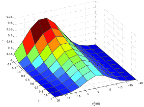
Figure 1: Blind channel estimation efficiency versus noise power and system load in moment-matching-based channel estimation

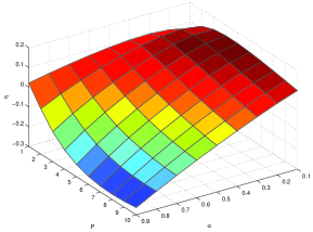
Figure 2: Blind channel estimation efficiency versus channel order and training symbol proportion in moment-matching-based channel estimation

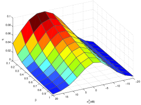
Figure 3: Blind channel estimation efficiency versus noise power and system load in subspace-based channel estimation

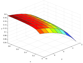
Figure 4: Blind channel estimation efficiency versus channel order and training symbol proportion in subspace-based channel estimation

References

References

- [1] S. E. Bensley and B. Aazhang, “Subspace-based channel estimation for code division multiple acess communication systems,” IEEE Trans. Commun., Vol. 44, pp. 1009-1020, Aug. 1996.
- [2] V. Buchoux, O. Cappe, E. Moulines and A. Gorokhov, “On the performance of semi-blind subspace-based channel estimation,” IEEE Trans. Signal Processing, Vol. 48, pp. 1750-1759, June 2000.
- [3] S. Buzzi and H. V. Poor, “Channel estimation and multiuser detection in long-code DS/CDMA systems,” IEEE J. Select. Areas Commun., Vol. 19, pp. 1476-1487, Aug. 2001.
- [4] B. Hassibi and B. M. Hochwald, “How much training is needed in multiple-antenna wireless links?,” IEEE Trans. Inform. Theory, Vol. 49, pp. 951-963, Apr. 2003.
- [5] H. Li and H. V. Poor, “Impact of channel estimation error on multiuser detection via the replica method ,” Proc. 2004 IEEE Global Telecomm. Conf., Dallas, TX, Nov. 30 - Dec. 2, 2004.
- [6] H. Li and H. V. Poor, “Performance analysis of semi-blind channel estimation in fading DS-CDMA channels,” submitted to IEEE Trans. Signal Process..
- [7] H. Liu, G. Xu, L. Tong and T. Kailath, “Recent developments in blind channel equalization: From cyclostationarity to subspaces,” Signal Processing, Vol. 50, pp. 83-99, Jan. 1996.
- [8] B. Porat, Digital Processing of Random Signals. Prentice Hall, Upper Saddle River, NJ, 1994.
- [9] W. Rudin, Principles of Mathematical Analysis. McGraw-Hill Inc., New York, NY, 1976.
- [10] J. Sun, Analysis of Matrix Perturbation. Science Press, Beijing, China, 2001.
- [11] Z. Xu and M. K. Tsatsanis, “Blind channel estimation for long code multiuser CDMA systems,” IEEE Trans. Signal Processing, Vol. 48, pp. 988-1001, Apr. 2000.
- [12] Z. Xu, “Effects of imperfect blind channel estimation on performance of linear CDMA receivers,” IEEE Trans. Signal Processing, Vol. 52, pp. 2873-2884, Oct. 2004.
- [13] H. H. Zeng and L. Tong, “Blind channel estimation using the second order statistics: Algorithms,” IEEE Trans. Signal Processing, Vol. 45, pp. 1919-1930, Aug. 1997.