Limits of Rush Hour Logic Complexity

Abstract

Rush Hour Logic was introduced in [2] as a model of computation inspired by the “Rush Hour” toy puzzle, in which cars can move horizontally or vertically within a parking lot. The authors show how the model supports polynomial space computation, using certain car configurations as building blocks to construct boolean circuits for a cpu and memory. They consider the use of cars of length 3 crucial to their construction, and conjecture that cars of size 2 only, which we’ll call Size 2 Rush Hour, do not support polynomial space computation. We settle this conjecture by showing that the required building blocks are constructible in Size 2 Rush Hour. Furthermore, we consider Unit Rush Hour, which was hitherto believed to be trivial, show its relation to maze puzzles, and provide empirical support for its hardness.

1 Introduction

Sliding block puzzles are among the simplest kind of motion planning problems. They involve moving rectangular pieces around inside a bigger rectangle with the goal of moving a specific piece to a specific target location. Problems of this kind were first proved to be PSPACE hard in [1] for arbitrarily large blocks, and later in [3] (or its journal version [4]) for fixed size blocks.

A collection of interactive sliding puzzles can be found at

http://johnrausch.com/SlidingBlockPuzzles/default.htm.

This paper focuses on the Rush Hour puzzle, featured at

http://www.puzzles.com/products/rushhour.htm,

and quoted as “one of the most elegant and fun sliding block puzzles to come on the market in years”. Its distinguishing characteristic is that the pieces, which are shaped as cars, can move only in their lengthwise direction, not sideways. The playing field is a ’parking lot’ of size 6 by 6, with only one exit, and with cars of size 2 by 1 and 3 by 1. The goal is to get a particular target car out of the lot through the exit. In [2], the computational complexity of ‘Generalized Rush Hour’, played on an arbitrarily large $m$ by $n$ board, is studied.

2 Rush Hour Computing

Flake and Baum hit upon the brilliant idea of partitioning the whole board into ‘blocks’ of constant size $k$ by $k$, which are bordered by walls of interlocking cars, leaving only one gap between adjacent blocks. Figure 1 shows four such blocks, each of size 11 by 11 (with some cars sticking out at the corners). Empty space is shown around the cars to make the cars stand out, which would not be present in the sliding block puzzle. The four black cars in the center, for example, are completely jammed in and unable to move. In fact we use black to denote cells that are always occupied by a car. Cars that can move back and forth one step only, are black at one end, and gray or striped at the other. The latter is used for chains of cars connecting the gaps.

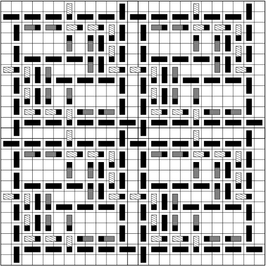
Figure 1: four blocks

Flake and Baum designed particular single block car configurations that behave as logical gates, imposing certain constraints on the 4 cars occupying the top, left, right, and bottom gaps of the block.

2.1 Functional vs Constraint Gates

Yet these gates are subtly different in behavior from classical boolean gates, which distinguish one or more inputs from the output. In classical circuits, the state of a gate’s output is uniquely determined by the state of its inputs, and wires must always connect an output of one gate to an input of another.

A Rush Hour block instead puts constraints on the combined states of its ‘ports’. Each port can be ‘in’ or ‘out’. The blocks in Figure 1 forbid the top and right port from both being ‘in’, and also the left and bottom port from both being ‘in’.

Consider two adjacent ports, $P$ and $Q$, of two adjacent blocks, for example the right port of the top-left block and the left port of the top-right block.

We can consider $P$ an output and $Q$ an input. The ‘in’ state of $P$ allows $Q$ to be in state ‘out’, which corresponds to an active wire $P\rightarrow Q$, since the top-right block now has more freedom of movement than if $Q$ were ‘in’.

On the other hand, if we consider $Q$ an output and $P$ an input, then the ‘out’ state of $Q$ forces $P$ to be in state ‘in’, which corresponds to an inactive wire $Q\rightarrow P$.

3 Nondeterministic Constraint Logic

Hearn and Demaine, in [3], abstracted the notion of constraining gates into the ‘Nondeterministic Constraint Logic’ model of computation. They propose a somewhat abstract graph formulation, as well as a more concrete circuit formulation for machines, and establish translations between the two. Below I introduce a new formulation which combines the formal rigor of the graph formulation with the concreteness of the circuit formulation. I believe the few extra definitions required in this formalism are offset by the conceptual simplicity and flexibility in gate design.

Basically, a machine is a circuit of gates and wires, where gates are nodes with labeled half-edges, and wires are a matching on half-edges. The half-edges take on the role of ports, and the ‘in’ or ‘out’ state of a port is naturally represented by directing the half-edge in or out.

3.1 Gate types

Definition 1

A gate type is a tuple $<L,S,E,o>$, where $L$ is a set of labels, $S$ a set of states, $E\subseteq S\times S$ a symmetric set of possible state transitions, and $o:S\rightarrow 2^{L}$ gives for each state $s$, an orientation of all half-edges. Transitions are only allowed between states that differ in the orientation of exactly one half-edge.

Figure 2: a WIRE gate

The simplest non-trivial type is the WIRE gate shown in Figure 2, which merely forbids its two half-edges to both be inward.

Figure 3: (a) gate type AND (b) usual representation (c) viewed as SPLIT

A more interesting type is the AND gate $<\{x,y,z\},S,E,o>$ whose states, transitions, and orientations are shown in Figure 3 (a). The usual representation of an AND gate in Figure 3 (b) emphasizes the role of $z$ as an output that can be active only when both inputs $x,y$ are, while the splitting wire emphasizes the role of $x,y$ as outputs that can be active only when input $z$ is.

Figure 4: (a) gate type OR (b) usual representation (c) symmetric view

Another type is the OR gate shown in Figure 4 (a). The usual representation in Figure 4 (b) arbitrarily shows $x,y$ as inputs and $z$ as output, but from (a) we can see that $x,y,z$ play equal roles, so a symmetric representation as in (c) is perhaps more appropriate.

Figure 5: (a) gate type HALF-OR (b) representation

Our last example is the HALF-OR gate shown in Figure 5 (a). This differs from the OR in having two states with both inputs and the output active. Consider the middle state where both inputs are active but the output inactive. Then to activate the output, a choice must be made of which input the output will depend on. That input then needs to remain active as long is the output is. For this reason it was called a ‘Latch’ in [3]. The next section shows the use of the HALF-OR gate.

3.2 Machines

A machine is basically a bunch of gates connected together:

Definition 2

A machine is an augmented graph in which all half-edges are labeled, and each node has a gate type consistent with the labels on its incident half-edges. Half-edges may remain unconnected; these are the input/output ports of the machine.

Definition 3

A machine state orients all half-edges, consistent across paired half-edges (one being ‘in’ and the other ‘out’), and assigns to each node a state of its gate type consistent with the incident half-edge orientations.

Figure 6: machine with one SPLIT and two HALF-OR gates.

A very simple machine, combining two HALF-ORs with a SPLIT gate, is shown in Figure 6. The fact that we matched same-labeled half-edges is done just for convenience, so that we may refer to the edges as $xx$, $yy$, or $zz$. We may wonder in what state the three unmatched half-edges can be, among all valid machine states. If $z$ is ‘in’, then the split requires both the $xx$ and $yy$ edges to be oriented downward to the half-ors. Since one HALF-OR must have an in-going $z$, this gate will require an out-going $x$ or $y$. This argument shows that not all three machine ports can be ‘in’. If this were the only restriction, then this machine would seem to behave as an OR gate. Figure 7 shows that this is indeed the case. To distinguish the two similarly oriented HALF-OR states, a line is drawn indicating the input on which the output is dependent. All 7 states of the OR gate can be achieved as part of states of the machine, and all 9 transitions are possible as a sequence of machine transitions. For example, from the middle top state, we can flip edge $zz$ twice to make the left HALF-OR dependent on $x$ instead of on $y$, allowing us to flip $yy$, and next flipping $xx$ yields the machine state at the middle left.

Figure 7: possible machine states and multi-step transitions

Machines thus allow us to compose new gate types from other ones. The fact that 2 HALF-ORs and a SPLIT make an OR was first noticed in an earlier version of this paper, and occurs in [3] as Lemma 5. Their convention about edge orientation is the opposite of ours though; a directed edge $s\rightarrow t$ in their paper means that the wire from output $s$ to input $t$ is active, while in our model it means that cars have moved out at $a$ and in at $t$, which, considered as a wire from output $s$ to input $t$, is inactive.

The main result of [3] is that Nondeterministic Constraint Logic, in particular the question of whether one machine state can change into another through a series of edge flips, is PSPACE complete. They even strengthen this to hold for ternary (degree 3) planar machines, by showing how a CROSSOVER, essentially a cross product of two WIREs as embedded in a plane, can be composed of ANDs and ORs.

This general result allows them to give an alternative proof to the [2] result that Rush Hour is PSPACE complete. They exhibit 7x7 blocks corresponding to gate types AND and HALF-OR, and then put 5x5 of these together to make superblocks for AND, HALF-OR, straight wire, and turning wire, from which arbitrary ternary planar machines may be built.

4 Size 2 Rush Hour

In this section we show our main result that

Theorem 1

Size 2 Rush Hour is PSPACE complete.

Just as [3] did for Size 2-or-3 Rush Hour, we prove this result by providing the building blocks to implement any planar ternary Nondeterministic Constraint Logic machine as an instance of Size 2 Rush Hour.

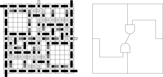
Figure 8: AND/SPLIT block

The block in Figure 8 implements 2 AND gates with their outputs matched. Omiting the car marked ’A’ has the effect of short-circuiting the top-right AND, leaving one with a single AND and one unconstrained port.

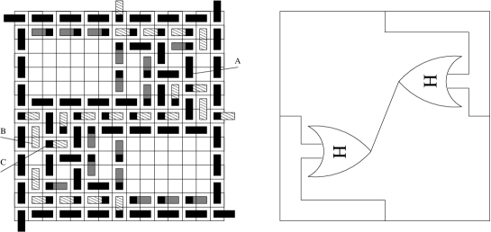
Figure 9: HALF-OR block

The block in Figure 8 implements 2 HALF-OR gates with their outputs matched. Note that car ‘C’ can be moved to the left only by locking in car ‘B’, either above or below it. This corresponds to the dependency we see in the HALF-OR state diagram.

Putting the car marked ’A’ in a horizontal position has the effect of short-circuiting the top-right HALF-OR, while leaving the top port unconstrained.

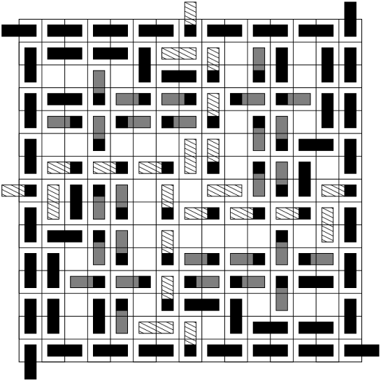
Figure 10: CROSSOVER block

The CROSSOVER block in Figure 10 was designed before the author learned of its redundancy. Still, it is rather amazing that it can be made to work in such limited space. In any case it provides us with a straight WIRE block, which, together with a stretched out version of the turning WIRE block in Figure 1, provides us with all the necessary plumbing to connect the logical gates together.

The proof is completed by verifying the correct operation of each block, which is greatly facilitated by the coloring. In particular, if it were possible to vacate any black colored cell, then one such cell would need to be vacated before any other, and it’s easy to manually verify that this is not possible.

A computer enumeration of all possible states of each block was used to verify correct operation.

5 Unit Size Rush Hour

Taking the constraint on car size to its extreme, we arrive at Unit Size Rush Hour, where every car occupies exactly one cell. An example instance is

||=
|-|
-.|

where ‘—’ denotes a vertical car, ‘-’ and ‘=’ denote horizontal cars, and ‘.’ an empty cell. The ‘=’ is the unique target car. The question is whether some sequence of car moves allows the target car to reach the left end of its row where it may exit the parking lot. For our example the answer is yes, as witnessed by the sequence of moves

 12   11   10    9    8    7    6    5    4    3    2    1    0
||=  ||=  ||=  ||=  |.=  |=.  |=|  |=|  |=|  |=|  |=|  .=|  =.|
|-|  |-|  .-|  -.|  -||  -||  -|.  -||  -||  -.|  .-|  |-|  |-|
-.|  .-|  |-|  |-|  |-|  |-|  |-|  |-.  |.-  ||-  ||-  ||-  ||-

Above each diagram is shown its distance-to-solve. In this case there is only one empty cell, which necessarily swaps places with a car on every move. This gives it the feel of a maze problem. In fact, consider

Definition 4

A Rush Hour Maze is a rectangular grid of cells one of which is the starting location for the player. The player can move either horizontally to a cell he last left horizontally, or vertically to a cell he last left vertically. Every cell except the start is oriented to restrict the first arrival. The exit of the maze is between two specified neighboring cells.

Then every Unit Rush Hour instance with one empty cell, in which the target is the leftmost horizontal car in its row is equivalent to a Rush Hour Maze instance. The exit is between the two leftmost cells on the target row. Having the maze player move between these two cells is equivalent to moving a horizontal car between the two cells. By assumption, this must be the target car reaching the exit.

Having the exit of a Rush Hour Maze between cells is important for ensuring non-triviality, since the question of whether the player can reach a given exit cell reduces to the following question:

In the directed graph that connects from each cell to neighbors of appropriate orientation, does there exist a path from the player to the exit cell?

This question can be answered with a straightforward depth-first search, thus all mazes with exit cells are rather trivial.

Similarly, the question of whether a specific car can be moved at all reduces to the existence of a path from the player to that car.

6 Right-hand rule

In plain mazes, one can sometimes follow a simple rule in order to find the exit. The Right-Hand Rule says to always take the rightmost turn, as pictured in Figure 11. It works in any maze whose underlying graph is acyclic.

Figure 11: solving a 4x4 maze using the right-hand rule

Also in Rush Hour Mazes, the right-hand rule is well defined. And indeed it is guaranteed to lead to the exit in case the state graph is acyclic. But whereas the states of a plain maze are readily apparent as the possible positions of the player, a Rush Hour Maze can have multiple states with the same player position, such as positions 3 and 9, or 22 and 32, below.

  0     3     9    12    14    22    32    36    44
||=-  ||=-  |=-|  |=-|  |=-|  |=-|  ||=-  .|=-  ||=-
|-|.  |-.|  ||.-  |.|-  |||-  |||-  |-||  |-||  |-|.
|--|  |-|-  |-|-  ||--  |-.-  --.|  --.|  |--|  |--|
---|  ---|  ---|  ---|  ---|  |---  |---  |---  ---|

The right-hand rule fails to find the “exit” here, having pushed the target car back between moves 22–32 leaving it out of reach in position 36.

7 Empirical Results

The most straightforward way to get a feel for the hardness of puzzles is to study how the worst-case solution length grows with the problem size. Superpolynomial growth is a prerequisite for hardness. In order to study solution length in small cases, we implemented an exhaustive state-space search program for Unit Rush Hour, focusing on instances with a single empty cell. Consider the graph $G$ of all possible configurations of width $w$ height $h$ and an exit on row $e$. With $wh$ possibilities for the location of the empty cell, and $2^{wh-1}$ possible orientations of the cars in the other cells, $G$ has $wh2^{wh-1}$ nodes, or states. Searching $G$ requires knowing which states we’ve visited before. Storing even one bit per state is undesirable since it would put the case $w=h=6$ out of reach at 144 Gbyte. Instead we partition $G$ as follows. First, we remove from $G$ all states with no horizontal cars on the exit row. In all remaining states, the leftmost car on the exit row is the target car. Depending on whether this car in the leftmost cell, a state is either solved or unsolved. Of the solved states, we only keep the justsolved ones, where the empty cell is right next to the target car. This partitions $G$ into many connected components, and preserves the largest distance to solution. We can now enumerate all justsolved states, checking if we’ve visited it before, and if not, search the whole connected component marking all encountered justsolved states as visited. This takes only $2^{wh-2}$ bits, which amounts to a feasible 2 Gbyte for $w=h=6$. Searching each component in a breadth first manner further helps to conserve space. The following table lists the worst-case solution length for each width and height, over all possible exit rows and states.

width	2	3	4	5	6	7	8	9	10
height
2	3	6	8	10	12	14	16	18	20
3	5	12	21	32	43	54	65	76	87
4	7	21	40	87	132	194	286	435
5	9	31	75	199	336	699
6	11	41	167	339	732
7	13	51	215	578
8	15	62	309
9	17	73	650
10	19	84

This limited data suggests an exponential growth rate. It is interesting to analyze these worst-case solutions in detail.

Figure 12 visualizes the 199 step solution of the hardest 5x5 instance.

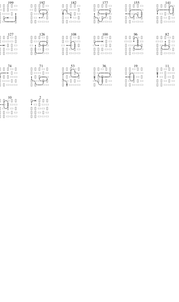
Figure 12: solution to hardest 5x5 instance

The thick lines indicate the changing position of the empty cell. Curiously, the solution can be broken down into segments each of which is either a simple path, or a path followed by a circuit, followed by the path in reverse. In the latter case, the effect of the segment is limited to flipping the orientation of all circuit corners, which somewhat resembles the flipping of a bit.

Figure 13 visualizes the 732 step solution of the hardest 6x6 instance.

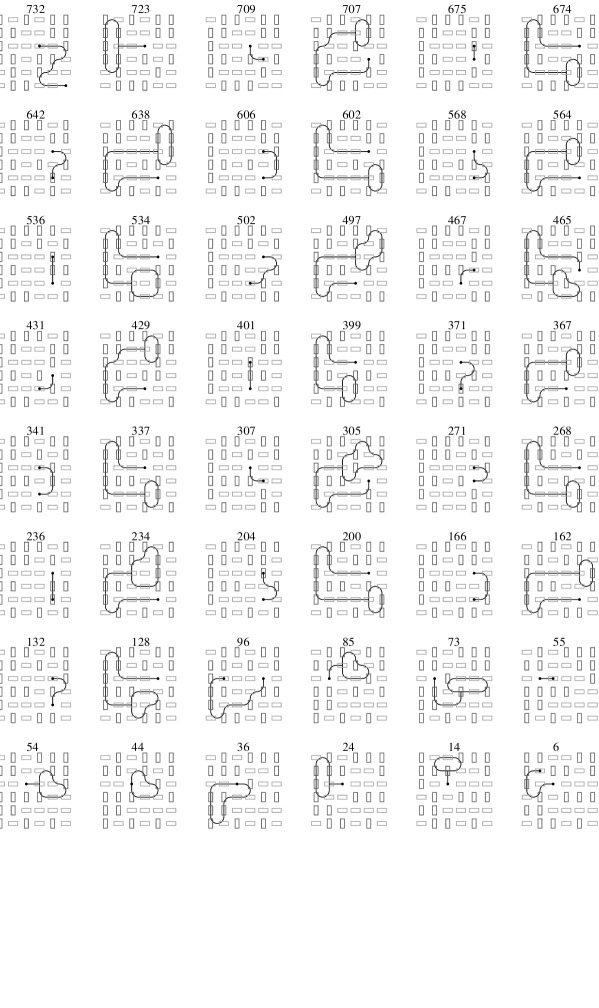
Figure 13: solution to hardest 6x6 instance

Here, we can also make out ‘virtual’ bit flips on a larger scale. Comparing the states at distances 674 and 268, we see that they differ in only the 4 corners of a ‘virtual’ circuit, taking no less than 406 steps to complete.

There’s little hope of exhaustively searching all 7x7 instances using our approach, as it would take $2^{49-2}$ bits, or 16 Tbyte. But already in the 6x6 case, a great deal of complexity is apparent.

What is far from apparent though, is how to harness this complexity in constructing particular circuits, such as binary counters that would prove the existence of exponential length solutions, or even the AND and OR gates that provide a basis for Nondeterministic Constraint Logic. This leaves us with many questions about the complexity of Unit Rush Hour.

8 Open Problems

While Size 2 Rush Hour was shown to be PSPACE complete, the complexity of Unit Rush Hour eludes us. It’s not clear if limiting the number of empty spaces to one reduces the complexity of Unit Rush Hour. Empirical results suggest that the hardest instances do in fact have only one empty space. Finally, it is possible that Unit Rush Hour becomes more complex if we can designate some of the cars as being neither horizontal nor vertical but plain immobile, which is equivalent to saying the parking lot can have arbitrarily shaped walls. Let’s call this generalization Walled Unit Rush Hour. Obviously, Rush Hour Maze is no harder than Unit Rush Hour, which in turn is no harder than Walled Unit Rush Hour. But this leaves us with a big open

Question 1

What is the complexity of Rush Hour Maze, Unit Rush Hour, and Walled Unit Rush Hour? Are they in P, PSPACE complete, or in between?

References

- [1] J.E. Hopcroft, J.T. Schwartz, and M. Sharir. On the Complexity of Motion Planning for Multiple Independent Objects: PSPACE-Hardness of the ’Warehouseman’s Problem’. International Journal of Robotics Research, 3(4):76–88, 1984.
- [2] Gary. W. Flake and Eric. B. Baum. Rush Hour is PSPACE-complete. Theoretical Computer Science, 270(1-2): 895–911, January 2002.
- [3] Robert A. Hearn and Erik D. Demaine. The Nondeterministic Constraint Logic Model of Computation: Reductions and Applications. in Proceedings of the 29th International Colloquium on Automata, Languages and Programming (ICALP 2002), Lecture Notes in Computer Science, volume 2380, Malaga, Spain, July 8-13, 2002, pages 401-413.
- [4] Robert A. Hearn and Erik D. Demaine. PSPACE-Completeness of Sliding-Block Puzzles and Other Problems through the Nondeterministic Constraint Logic Model of Computation. Theoretical Computer Science, to appear in 2004.