Nonlinear MMSE Multiuser Detection Based on
Multivariate Gaussian Approximation

Abstract

In this paper, a class of nonlinear MMSE multiuser detectors are derived based on a multivariate Gaussian approximation of the multiple access interference. This approach leads to expressions identical to those describing the probabilistic data association (PDA) detector, thus providing an alternative analytical justification for this structure. A simplification to the PDA detector based on approximating the covariance matrix of the multivariate Gaussian distribution is suggested, resulting in a soft interference cancellation scheme. Corresponding multiuser soft-input, soft-output detectors delivering extrinsic log-likelihood ratios are derived for application in iterative multiuser decoders. Finally, a large system performance analysis is conducted for the simplified PDA, showing that the bit error rate performance of this detector can be accurately predicted and related to the replica method analysis for the optimal detector. Methods from statistical neuro-dynamics are shown to provide a closely related alternative large system prediction. Numerical results demonstrate that for large systems, the bit error rate is accurately predicted by the analysis and found to be close to optimal performance.

1 Introduction

It is well-known that the computational complexity of individually optimal detection for direct-sequence code-division multiple-access (CDMA) grows exponentially with the number of users [1], as the computation of the marginal posterior-mode (MPM) distribution is required. Maximum a posteriori probability (MAP) detection for each user is therefore far too complex for practical CDMA systems with even a moderate number of users. The exponentially growing complexity has inspired a considerable effort in finding low complexity suboptimal alternatives capable of resolving the detrimental effects of multiple-access interference (MAI).

Interference cancellation (IC) strategies have been subject to particular attention due to low complexity, a simple modular structure and competitive performance [2]. Early work was focused on linear cancellation and hard decision cancellation [3, 4]. More recently, soft decision cancellation have been shown to provide performance improvements. In [5] it was shown that soft decision cancellation based on convex projections provides an iterative solution to the convex-constrained multiuser maximum-likelihood problem. The well-known result that the optimal nonlinear minimum mean squared error (MMSE) estimate is the conditional posterior-mode mean was used in [6] for a decision-feedback receiver. Similar arguments were used in [7] to arrive at a soft decision IC structure, and the same structure was derived in [8] based on neural networks arguments. Even though this cancellation structure has a low complexity of order $\mathcal{O}(K^{2})$, numerical examples show that near single-user performance can be achieved for large systems [8].

In [9], the probabilistic data association (PDA) method was introduced for multiuser detection as a low complexity nonlinear alternative. The decision statistics of the users are modelled as binary random variables where the MAI is approximated as multivariate Gaussian noise. The a posteriori probability (APP) for the data symbols of each user is updated sequentially given the associated APPs of all other users. Although this scheme has a low computational complexity of order $\mathcal{O}(K^{3})$, it can achieve near single-user performance for systems with a moderate number of users [9].

The most celebrated multiuser detectors applied for iterative multiuser decoding of coded CDMA are based on linear filtering, e.g., [10, 11, 12, 13, 14, 15, 16, 17]. Parallel IC (PIC) and linear MMSE filtered PIC were investigated in [10, 11, 12] and [13, 14], respectively. In [15], it was observed that for low-complexity detectors, information combining over iterations can be rewarding, providing performance and system load gains. The partial cancellation structure in [15] was justified in [16] as recursive maximal ratio combining over all previous iterations, while a more complicated vector Kalman filter applied across iterations was presented in [17]. Nonlinear multiuser detectors based on list detection have been developed for iterative multiuser decoding and shown to provide equally impressive performance gains at low complexity [18]. As the PDA detector generates APPs directly, it has been applied for iterative multiuser decoding with only minor modifications, also demonstrating competitive gains [19].

Large system performance analysis techniques from statistical mechanics and statistical neuro-dynamics have been applied successfully for performance analysis of some multiuser detectors. In [20], the performance of the optimal multiuser detector was analyzed based on the replica method. This approach has further been developed in [21], and in [22] for coded CDMA. A different approach inspired by statistical neuro-dynamics was used in [23] to arrive at a large system analysis for a belief propagation (BP) multiuser detector. Methods from statistical neuro-dynamics [24, 25] have also been applied in [26] for large system analysis of PIC.

In this paper, a class of nonlinear MMSE (NMMSE) multiuser detectors are derived based on a multivariate Gaussian approximation of the MAI. The computation of the NMMSE estimate requires a sum of terms, which grows exponentially in numbers with the number of users. Using the multivariate Gaussian approximation, this summation is replaced by integration, reducing the complexity significantly. The expressions describing this approach is shown to be identical to the description of the PDA detector in [9], thus providing an alternative analytical justification.

A simplification to the NMMSE/PDA detector, based on approximating the covariance matrix of the multivariate Gaussian distribution with a diagonal, is suggested. The corresponding soft interference cancellation scheme is similar to the IC structure of the detectors in [7, 8]and can be implemented in parallel or serially. The corresponding complexity is of the order of IC, namely $\mathcal{O}(K^{2})$ as compared to the PDA with an order of complexity of $\mathcal{O}(K^{3})$.

Multiuser soft-input, soft-output (SISO) detectors delivering extrinsic log-likelihood ratios (LLRs) at the output are derived from the class of NMMSE-based detectors. The multiuser SISO detectors are applied for iterative multiuser decoding of coded CDMA and found to converge to single-user performance at loads larger than linear multiuser SISO alternatives.

Finally, a large system performance analysis is conducted for the simplified PDA. In the large system limit, the bit error rate performance of this detector can be accurately predicted and related to the replica method analysis for the optimal detector [20]. Methods from statistical neuro-dynamics can also be used for a closely related alternative large system prediction [23, 24]. It follows that the simplified PDA has the same predicted large system performance as the optimal detector. Numerical results show that for large systems, the bit error rate (BER) is accurately predicted by the analysis and found to be close to optimal performance.

The paper is organized as follows. In Section 2, the uncoded and coded CDMA discrete-time models are presented together with the standard iterative multiuser decoding structure. In Section 3 nonlinear minimum mean squared error estimation, leading to the marginal posterior-mode (MPM) decision, is briefly reviewed providing the setting for the multivariate Gaussian approximation considered in Section 4. The simplified PDA is derived in Section 5, while the corresponding NMMSE-based multiuser SISO detectors are detailed in Section 6. The large system analysis of the simplified PDA is derived in Section 7, numerical results are presented in Section 8 and concluding remarks are summarized in Section 9.

2 System Model

An elaborate discrete-time system model for CDMA is developed from first principles in [27]. The discrete-time model described below is a simplified, special case of this general model. For simplicity, assume a symbol-synchronous CDMA system with $K$ users, binary data symbols and binary spreading with processing gain $N$. Random spreading is assumed where each binary chip is modulated onto a common chip waveform for transmission. The output of a bank of $K$ chip-matched filters is given by

$${\mathbf{r}}=[{\mathbf{s}}_{1},...,{\mathbf{s}}_{k},...,{\mathbf{s}}_{K}]\;{\mathbf{d}}+{\mathbf{n}}={\mathbf{S}}{\mathbf{d}}+{\mathbf{n}},$$ (1)

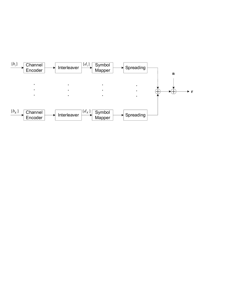
where ${\mathbf{S}}\in\{\pm 1/\sqrt{N}\}^{N\times K}$ is the spreading matrix, ${\mathbf{d}}\in\{\pm 1\}^{K}$ is the data symbol vector, ${\mathbf{n}}$ is a zero-mean additive white Gaussian noise (AWGN) vector with covariance matrix $\sigma^{2}{\mathbf{I}}$, and $N_{0}=2\sigma^{2}$ is the one-sided spectral density of the white Gaussian noise. The model is illustrated in Figure 1 within the error control coded model.

Figure 1: Discrete-time model for coded CDMA.

Some notation that will prove useful later on. At chip interval $\mu$, the received signal is described by $r_{\mu}=\sum_{k=1}^{N}s_{\mu k}d_{k}+n_{\mu}$, where $r_{\mu}$, $s_{\mu k}$ and $n_{\mu}$ are corresponding elements of the vectors ${\mathbf{r}}$, ${\mathbf{s}}_{k}$ and ${\mathbf{n}}$, respectively. In addition, let ${\mathbf{S}}_{k}=[{\mathbf{s}}_{1},...,{\mathbf{s}}_{k-1},{\mathbf{s}}_{k+1},...,{\mathbf{s}}_{K}]$ be the spreading matrix with column $k$ removed. The model in (1) can be further developed to include bit-level matched filtering as ${\mathbf{y}}={\mathbf{S}}^{\scriptscriptstyle\text{T}}{\mathbf{r}}={\mathbf{R}}{\mathbf{d}}+{\mathbf{z}}$, where $\mathsf{E}\{{\mathbf{z}}{\mathbf{z}}^{\scriptscriptstyle\text{T}}\}=\sigma^{2}{\mathbf{R}}$. It follows that $y_{k}=\sum_{j=1}^{K}R_{kj}d_{j}+z_{k}$, where $y_{k}$ and $z_{k}$ are respective elements of vectors ${\mathbf{y}}$ and ${\mathbf{z}}$, while $R_{kj}$ is the corresponding element of the matrix ${\mathbf{R}}$.

When error control coding is introduced, the model is extended as shown in Figure 1. Now the binary data symbols are encoded, interleaved and mapped onto a binary phase-shift keying constellation in order to arrive at the code symbol vector ${\mathbf{d}}$, which corresponds to the data symbol vector in the model for the uncoded case. 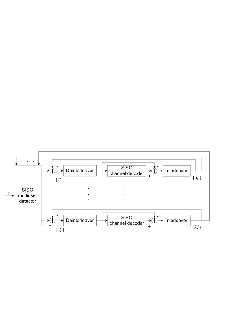In this paper, we consider iterative multiuser decoding for the coded case with the corresponding decoding structure shown in Figure 2.

Figure 2: General structure for iterative multiuser decoding.

A multiuser SISO detector computes extrinsic LLRs of the code bits for all the users based on the received signal and a priori LLRs of the code bits. The extrinsic LLRs of user $k$ are deinterleaved and input to an APP decoder for the error control code applied by user $k$. This single-user decoder outputs extrinsic LLRs, which are interleaved and, together with extrinsic LLRs of all the other users, forwarded to the multiuser SISO as a priori LLRs for the next iteration. This type of iterative multiuser decoder is a direct application of the turbo decoding principle and commonly used for iterative multiuser decoding [13, 19, 22, 17].

3 Nonlinear MMSE Estimation

Let the nonlinear MMSE data estimate for user $k$ be denoted as $m_{k}=\mathsf{g}^{*}(d_{k},{\mathbf{r}})$, where $\mathsf{g}^{*}(d_{k},{\mathbf{r}})$ is the nonlinear function that minimizes the mean squared error $\mathsf{E}\{(d_{k}-\mathsf{g}(d_{k},{\mathbf{r}}))^{2}\}$. In order to find the optimal nonlinear function, the mean squared error is expressed as an expectation of a conditional expected value $\mathsf{E}\{\mathsf{E}\{(d_{k}-\mathsf{g}(d_{k},{\mathbf{r}}))^{2}|{\mathbf{r}}\}\}$ [28]. Since the inner expectation is always positive, the minimum is achieved by:

$$\min_{\mathsf{g}(d_{k},{\mathbf{r}})\in\mathbb{G}}\mathsf{E}\{[d_{k}-\mathsf{g}(d_{k},{\mathbf{r}})]^{2}|{\mathbf{r}}\}=\min_{\mathsf{g}(d_{k},{\mathbf{r}})\in\mathbb{G}}\sum_{d_{k}=\pm 1}[d_{k}-\mathsf{g}(d_{k},{\mathbf{r}})]^{2}\mathsf{Pr}(d_{k}|{\mathbf{r}}),$$ (2)

where $\mathbb{G}$ is the relevant set of nonlinear functions. The solution is the conditional mean $\mathsf{E}\{\mathsf{Pr}(d_{k}|{\mathbf{r}})\}$ [28], leading to

$$m_{k}=\mathsf{g}^{*}(d_{k},{\mathbf{r}})=\sum_{d_{k}=\pm 1}d_{k}\mathsf{Pr}(d_{k}|{\mathbf{r}})=\sum_{{\mathbf{d}}\in\{-1,+1\}^{K}}d_{k}\mathsf{Pr}({\mathbf{d}}|{\mathbf{r}}).$$ (3)

Note that the polarity of $m_{k}$ in eqn. (3) is in fact the marginal posterior-mode decision, i.e.,

$$d_{k}^{*}=\arg\,\,\max_{d_{k}=\pm 1}\mathsf{Pr}(d_{k}|{\mathbf{r}})=\mathsf{sign}\left\{\sum_{{\mathbf{d}}\in\{-1,+1\}^{K}}d_{k}\mathsf{Pr}({\mathbf{d}}|{\mathbf{r}})\right\}.$$

Based on eqns. (2) and (3), the NMMSE data estimates for all the users can be described by a set of $K$ optimization problems:

$$m_{k}=\arg\min_{\tilde{m}_{k}\in\mathbb{R}}\sum_{d_{k}}(d_{k}-\tilde{m}_{k})^{2}\mathsf{Pr}(d_{k}|{\mathbf{r}}),\hskip 14.22636pt\text{for }k=1,2,...,K,$$

where $m_{k}$ is the NMMSE data estimate for user $k$. The $K$ problems can be solved independently since $\mathsf{Pr}(d_{k}|{\mathbf{r}})$ can be computed independently for each user.

Following Bayes’ rule, the marginal posterior-mode distribution can be found as

$$\mathsf{Pr}(d_{k}|{\mathbf{r}})=\frac{\mathsf{Pr}(d_{k})\mathsf{p}({\mathbf{r}}|d_{k})}{\sum_{d_{k}}\mathsf{Pr}(d_{k})\mathsf{p}({\mathbf{r}}|d_{k})}.$$ (4)

Here, the probability density function (pdf) $\mathsf{p}({\mathbf{r}}|d_{k})$ is found as a sum over $2^{K-1}$ terms as follows:

$$\mathsf{p}({\mathbf{r}}|d_{k})=\sum_{{\mathbf{d}}\backslash d_{k}\in\{-1,+1\}^{K-1}}\mathsf{p}({\mathbf{r}}|{\mathbf{d}})\mathsf{Pr}({\mathbf{d}}\backslash d_{k}),$$ (5)

where ${\mathbf{d}}\backslash d_{k}$ denotes a vector containing all the elements in ${\mathbf{d}}$ except $d_{k}$. This approach is however impractical for large system loads, as the computational complexity grows exponentially with the number of users. As an alternative, a multivariate Gaussian approximation is introduced below.

4 Multivariate Gaussian Approximation

Consider the received signal at chip level. The conditional pdf at chip interval $\mu$ is

$$\mathsf{p}(r_{\mu}|{\mathbf{d}})=\frac{\mathsf{exp}\left[-\frac{1}{2\sigma^{2}}\left(r_{\mu}-s_{\mu k}d_{k}-\Delta_{\mu k}\right)^{2}\right]}{\sqrt{2\pi\sigma^{2}}},$$

where $\Delta_{\mu k}=\sum_{l\neq k}s_{\mu l}d_{l}$ is the corresponding MAI. The conditional symbol-level pdf in (5) can then be expressed as

$$\mathsf{p}({\mathbf{r}}|d_{k}) = \sum_{{\mathbf{d}}\backslash d_{k}\in\{-1,+1\}^{K-1}}\prod_{\mu=1}^{N}\mathsf{p}(r_{\mu}|{\mathbf{d}})\mathsf{Pr}({\mathbf{d}}\backslash d_{k})$$ (6)

$$= \sum_{{\mathbf{d}}\backslash d_{k}\in\{-1,+1\}^{K-1}}\mathsf{Pr}({\mathbf{d}}\backslash d_{k})\frac{\mathsf{exp}\left[-\frac{1}{2\sigma^{2}}\left\|{\mathbf{r}}-{\mathbf{s}}_{k}d_{k}-\Delta_{k}\right\|^{2}\right]}{(2\pi\sigma^{2})^{N/2}},$$

where ${\mathbf{\boldsymbol{\Delta}}}_{k}=[\Delta_{1k},...,\Delta_{Nk}]^{\scriptscriptstyle\text{T}}$ is a vector for user $k$, containing the MAI contributions for each chip interval.

To reduce complexity, the probability distribution function of the random variable vector ${\mathbf{\boldsymbol{\Delta}}}_{k}$ is approximated by a multivariate Gaussian pdf. The summation in (6) can thus be replaced by an $N$-fold integration over the support of ${\mathbf{\boldsymbol{\Delta}}}_{k}$

$$\mathsf{p}({\mathbf{r}}|d_{k})\approx\int_{-\infty}^{\infty}\ldots\int_{-\infty}^{\infty}\mathsf{p}({\mathbf{r}},{\mathbf{\boldsymbol{\Delta}}}_{k}|d_{k})\,d{\mathbf{\boldsymbol{\Delta}}}_{k}=\int_{-\infty}^{\infty}\ldots\int_{-\infty}^{\infty}\prod_{\mu=1}^{N}\mathsf{p}(r_{\mu}|\Delta_{\mu k},d_{k})\mathsf{p}({\mathbf{\boldsymbol{\Delta}}}_{k})\,d{\mathbf{\boldsymbol{\Delta}}}_{k},$$ (7)

where $d{\mathbf{\boldsymbol{\Delta}}}_{k}=\prod_{\mu=1}^{N}d\Delta_{\mu k}$ denotes differentials for integration. The multivariate Gaussian pdf is described as follows. Since $\Delta_{\mu k}=\sum_{l\neq k}s_{\mu l}d_{l}$, it is reasonable to assume that the corresponding mean and covariance are

$$u_{\mu k}=\mathsf{E}\left\{\Delta_{\mu k}\right\}=\sum_{l\neq k}s_{\mu l}m_{l}$$

and

$$\mathsf{Cov}\left\{\Delta_{\mu k}\Delta_{\nu k}\right\} = \mathsf{E}\left\{\Delta_{\mu k}\Delta_{\nu k}\right\}-\mathsf{E}\left\{\Delta_{\mu k}\right\}\mathsf{E}\left\{\Delta_{\nu k}\right\}$$ (8)

$$= \sum_{j\neq k}s_{\mu j}s_{\nu j}(1-m_{j}^{2})+\sum_{j\neq k}\,\sum_{l\neq j,k}s_{\mu j}s_{\nu l}\left(\mathsf{E}\left\{d_{j}d_{l}\right\}-m_{j}m_{l}\right).$$

In the second term in (8), the expectation $\mathsf{E}\left\{d_{j}d_{l}\right\}$ must be computed. This computation has a complexity of the order of $\mathcal{O}(K^{2})$. To reduce complexity, the second term is omitted in the following. As $K$ grows large, it is expected that $\mathsf{E}\left\{d_{j}d_{l}\right\}\rightarrow m_{j}m_{l}$ and thus, the second term becomes negligible. The effect of removing this term is considered in Section 8 using numerical examples. With this simplification, the covariance matrix of ${\mathbf{\boldsymbol{\Delta}}}_{k}$ is reduced to

$${\mathbf{\boldsymbol{\Omega}}}_{k}=\mathsf{Cov}\{{\mathbf{\boldsymbol{\Delta}}}_{k}{\mathbf{\boldsymbol{\Delta}}}_{k}^{\scriptscriptstyle\text{T}}\}=\sum_{l\neq k}(1-m_{l}^{2}){\mathbf{s}}_{l}{\mathbf{s}}_{l}^{\scriptscriptstyle\text{T}}={\mathbf{S}}_{k}\mathsf{Diag}[{\mathbf{1}}-{\mathbf{m}}_{k}\circ{\mathbf{m}}_{k}]{\mathbf{S}}_{k}^{\scriptscriptstyle\text{T}},$$

where $\mathsf{Cov}\{\Delta_{\mu k}\Delta_{\nu k}\}=\sum_{l\neq k}s_{\mu l}s_{\nu l}(1-m_{l}^{2})$, ${\mathbf{m}}_{k}=[m_{1},m_{2},...,m_{k-1},m_{k+1},...,m_{N}]^{\scriptscriptstyle\text{T}}$ and ${\mathbf{a}}\circ{\mathbf{b}}$ denotes the Hadamard-product [29] of vectors ${\mathbf{a}}$ and ${\mathbf{b}}$, respectively. The multivariate Gaussian pdf of ${\mathbf{\boldsymbol{\Delta}}}_{k}$ is then

$$\mathsf{p}({\mathbf{\boldsymbol{\Delta}}}_{k})=\frac{\mathsf{exp}\left[-\frac{1}{2}({\mathbf{\boldsymbol{\Delta}}}_{k}-{\mathbf{u}}_{k})^{\scriptscriptstyle\text{T}}{\mathbf{\boldsymbol{\Omega}}}_{k}^{-1}({\mathbf{\boldsymbol{\Delta}}}_{k}-{\mathbf{u}}_{k})\right]}{(2\pi)^{N/2}\sqrt{\mathsf{det}[{\mathbf{\boldsymbol{\Omega}}}_{k}]}},$$

where ${\mathbf{u}}_{k}=[u_{1k},u_{2k},...,u_{Nk}]^{\scriptscriptstyle\text{T}}={\mathbf{S}}_{k}{\mathbf{m}}_{k}$.

Substituting this into (7) and performing the $N$-fold integration yields

$$\mathsf{p}({\mathbf{r}}|d_{k}) \varpropto \exp\left\{-\frac{1}{2}\left({\mathbf{r}}-{\mathbf{s}}_{k}d_{k}-{\mathbf{u}}_{k}\right)^{\scriptscriptstyle\text{T}}({\mathbf{\boldsymbol{\Omega}}}_{k}+\sigma^{2}{\mathbf{I}})^{-1}\left({\mathbf{r}}-{\mathbf{s}}_{k}d_{k}-{\mathbf{u}}_{k}\right)\right\}$$ (9)

$$\varpropto \exp\left\{d_{k}\left({\mathbf{r}}-{\mathbf{u}}_{k}\right)^{\scriptscriptstyle\text{T}}{\mathbf{C}}_{k}^{-1}{\mathbf{s}}_{k}\right\}=\mathsf{exp}\left\{d_{k}{\mathbf{s}}^{\scriptscriptstyle\text{T}}_{k}{\mathbf{C}}_{k}^{-1}\left({\mathbf{r}}-{\mathbf{S}}_{k}{\mathbf{m}}_{k}\right)\right\},$$

where ${\mathbf{C}}_{k}={\mathbf{\boldsymbol{\Omega}}}_{k}+\sigma^{2}{\mathbf{I}}$. It follows that the NMMSE estimate is given by

$$m_{k} = \sum_{d_{k}=\pm 1}d_{k}\mathsf{Pr}(d_{k}|{\mathbf{r}})=\sum_{d_{k}=\pm 1}d_{k}\frac{\mathsf{Pr}(d_{k})\mathsf{p}({\mathbf{r}}|d_{k})}{\sum_{d_{k}}\mathsf{Pr}(d_{k})\mathsf{p}({\mathbf{r}}|d_{k})}$$ (10)

$$= \mathsf{tanh}\left[\lambda_{k}^{p}/2+{\mathbf{s}}^{\scriptscriptstyle\text{T}}_{k}{\mathbf{C}}_{k}^{-1}\left({\mathbf{r}}-{\mathbf{S}}_{k}{\mathbf{m}}_{k}\right)\right],$$

where $\lambda_{k}^{p}=\mathsf{log}[\mathsf{Pr}(d_{k}=1)/\mathsf{Pr}(d_{k}=-1)]$ is the a priori log-likelihood ratio (LLR).

The above detector is know as the PDA detector, first suggested in [9]. Our contribution is to relate the PDA detector to the NMMSE estimation problem, which shows that the corresponding output is an approximation to the conditional a posteriori mean. Also, it is clear from (10) that the PDA detector corresponds to a nonlinear, filtered IC structure.

Solving the nonlinear system of equations in (10) requires a computational complexity of the order of ${\mathcal{O}}(K^{3})$ [9], where the complexity is dominated by the inversion of ${\mathbf{C}}_{k}$. A simplified approach is suggested below, approximating ${\mathbf{C}}_{k}$ with a diagonal matrix.

5 Simplified Probabilistic Data Association Detection

For large systems, the diagonal elements of ${\mathbf{C}}_{k}$ are dominant, encouraging the following approximation ${\mathbf{C}}_{k}=({\mathbf{\boldsymbol{\Omega}}}_{k}+\sigma^{2}{\mathbf{I}})\approx(\sigma_{k}^{2}+\sigma^{2}){\mathbf{I}}$, where $\sigma_{k}^{2}=\alpha(1-Q)$ with $\alpha=K/N$ being the system load and $Q=(1/K)\sum_{k}m_{k}^{2}$. The conditional pdf (9) is then simplified to

$$\mathsf{p}({\mathbf{r}}|d_{k}) = \prod_{\mu=1}^{N}\frac{\mathsf{exp}\left[-\frac{(r_{\mu}-s_{\mu k}d_{k}-u_{\mu k})^{2}}{2(\sigma_{k}^{2}+\sigma^{2})}\right]}{\sqrt{2\pi(\sigma_{k}^{2}+\sigma^{2})}}=\frac{\mathsf{exp}\left[-\frac{\left\|{\mathbf{r}}-{\mathbf{s}}_{k}d_{k}-{\mathbf{S}}_{k}{\mathbf{m}}_{k}\right\|^{2}}{2(\sigma_{k}^{2}+\sigma^{2})}\right]}{\left[(2\pi(\sigma_{k}^{2}+\sigma^{2})\right]^{N/2}}$$ (11)

$$\varpropto \mathsf{exp}\left[\frac{d_{k}{\mathbf{s}}^{\scriptscriptstyle\text{T}}_{k}\left({\mathbf{r}}-{\mathbf{S}}_{k}{\mathbf{m}}_{k}\right)}{\sigma_{k}^{2}+\sigma^{2}}\right],$$

which leads to

$$m_{k}=\mathsf{tanh}\left[\frac{\lambda_{k}^{p}}{2}+\frac{{\mathbf{s}}^{\scriptscriptstyle\text{T}}_{k}\left({\mathbf{r}}-{\mathbf{S}}_{k}{\mathbf{m}}_{k}\right)}{\sigma_{k}^{2}+\sigma^{2}}\right]=\mathsf{tanh}\left[\frac{\lambda_{k}^{p}}{2}+\frac{y_{k}-\sum_{j\neq k}R_{kj}m_{j}}{\sigma_{k}^{2}+\sigma^{2}}\right].$$ (12)

Note that (12) is similar to the iterative soft-decision multi-stage interference cancellation (MIC) scheme suggested independently in [6, 8, 7]. The MIC is described by

$$m_{k}=\mathsf{tanh}\left[\frac{\lambda_{k}^{p}}{2}+\frac{y_{k}-\sum_{j\neq k}R_{kj}m_{j}}{\sigma^{2}+\sum_{j\neq k}R_{kj}^{2}(1-m_{j}^{2})}\right].$$ (13)

For large $K$ and $N$, the term $\sum_{j\neq k}R_{kj}^{2}(1-m_{j}^{2})$ is well approximated by $\alpha(1-Q)$, using the fact that $\mathsf{E}\left\{R_{kj}^{2}\right\}=1/N$.

A simple way to solve (12) is by iteration over all users from an initial solution ${\mathbf{m}}^{0}$. This can be done in parallel as

$$m_{k}^{t+1}=\omega m_{k}^{t}+(1-\omega)\mathsf{tanh}\left[\frac{\lambda_{k}^{p}}{2}+\frac{y_{k}-\sum_{j\neq k}R_{kj}m_{j}^{t}}{\sigma^{2}+\alpha(1-Q^{t})}\right],$$ (14)

where superscript $t$ denotes the corresponding variable at iteration $t$. Also, $0\leq\omega<1$ is a weighting factor which improves the convergence properties of the parallel iteration in (14). Similar weighting factor approaches have been applied to linear cancellation and convex-constrained cancellation in [30, 5].

The fixed-point problem in (12) can also be solved with a serial iteration as

$$m_{k}^{t+1}=\omega m_{k}^{t}+(1-\omega)\mathsf{tanh}\left[\frac{\lambda_{k}^{p}}{2}+\frac{y_{k}-\sum_{j=1}^{k-1}R_{kj}m_{j}^{t+1}-\sum_{j=k+1}^{K}R_{kj}m_{j}^{t}}{\sigma^{2}+\alpha\left\{1-\frac{1}{K}\left[\sum_{j=1}^{k-1}(m_{j}^{t+1})^{2}+\sum_{j=k}^{K}(m_{j}^{t})^{2}\right]\right\}}\right].$$ (15)

It should be noted that convergence is not assured in general. However, for a series of numerical experiments, it has been observed that the serial implementation with $\omega=0$ always converged while a nonzero weighting factor is required for the parallel case to ensure convergence.

In the following, the parallel implementation in (14) is denoted as the parallel simplified PDA (PSPDA) and the serial implementation in (15) is denoted as the serial simplified PDA (SSPDA).

6 Multiuser Decoding

The multiuser detectors considered in this paper are based directly on estimating the marginal-mode probability distribution function. This feature makes these detectors well suited for low-complexity iterative multiuser decoding, requiring only minor modifications. Based on the general iterative multiuser decoding approach in [13, 19, 22], the extrinsic LLRs of the detectors developed above are derived.

¿From (4), the LLR for user $k$ based on the marginal mode probability distribution is

$$\Lambda^{\text{APP}}_{k}=\mathsf{log}\frac{\mathsf{Pr}(d_{k}=1|{\mathbf{r}})}{\mathsf{Pr}(d_{k}=-1|{\mathbf{r}})}=\mathsf{log}\frac{\mathsf{Pr}(d_{k}=1)\mathsf{p}({\mathbf{r}}|d_{k}=1)}{\mathsf{Pr}(d_{k}=-1)\mathsf{p}({\mathbf{r}}|d_{k}=-1)}=\lambda^{p}_{k}+\lambda^{e}_{k},$$

where $\lambda^{p}_{k}$ is the a priori LLR and $\lambda^{e}_{k}=\mathsf{log}\frac{\mathsf{p}({\mathbf{r}}|d_{k}=1)}{\mathsf{p}({\mathbf{r}}|d_{k}=-1)}$ is the extrinsic LLR for user $k$. A multiuser SISO based on the PDA detector is determined from (9). The corresponding LLR is $\lambda^{e}_{k}=2{\mathbf{s}}^{\scriptscriptstyle\text{T}}_{k}{\mathbf{C}}^{-1}_{k}\left({\mathbf{r}}-{\mathbf{S}}_{k}{\mathbf{m}}_{k}\right)$, following a sufficient number of iterations of the PDA detector, according to (10) either in parallel or serially. This is to arrive at as good an approximation as possible to the conditional a posteriori mean. Considering the approximate conditional pdf in (11), the corresponding LLR for a multiuser SISO based on the simplified PDA detector is $\lambda^{e}_{k}=\frac{2{\mathbf{s}}^{\scriptscriptstyle\text{T}}_{k}\left({\mathbf{r}}-{\mathbf{S}}_{k}{\mathbf{m}}_{k}\right)}{\sigma_{k}^{2}+\sigma^{2}}$, again assuming sufficient iterations of (14) or (15) to get a good approximation to ${\mathbf{m}}_{k}$ for all $k$.

Note that we now have two separate iterations, namely the overall multiuser decoding iteration, exchanging LLRs between the multiuser SISO and the bank of single-user APP decoders, and the internal NMMSE-detector iteration, improving the NMMSE estimate. A further design parameter is the choice of the initial solution ${\mathbf{m}}^{0}$. Typical choices are ${\mathbf{m}}^{0}=\mathbf{0}$, ${\mathbf{m}}^{0}={\mathbf{S}}^{\scriptscriptstyle\text{T}}{\mathbf{r}}$ or $m^{0}_{k}=\mathsf{tanh}\left[\lambda_{k}^{p}/2\right]$, $k=1,2,...,K$, using the most recent prior LLR for user $k$.

The performance of the proposed multiuser SISO detectors within an iterative multiuser decoder is evaluated based on numerical examples in Section 8.

7 Large System Performance Analysis

In this section, large system analysis is considered for the uncoded case. The BER performance of the PSPDA detector in (14) with uniform binary priors (i.e., $\lambda^{p}_{k}/2=0$) and ${\mathbf{m}}^{0}={\mathbf{0}}$ is investigated using an approach similar to [23, 26].

Let $h_{k}^{t}=A^{t}\left(y_{k}-\sum_{j\neq k}R_{kj}m_{j}^{t}\right)$, where $A^{t}=[\sigma^{2}+\alpha\left(1-Q^{t}\right)]^{-1}$. We can then express (14) as

$$m_{k}^{t+1}=\omega m_{k}^{t}+(1-\omega)\mathsf{tanh}\left[h_{k}^{t}\right]=\sum_{\kappa=0}^{t}\rho^{t-\kappa}\mathsf{tanh}\left[h_{k}^{\kappa}\right],$$ (16)

where the recursion in (14) has been repeatedly applied such that,

$$\rho^{t-\kappa}=\left\{\begin{array}[]{cl}\omega^{t-1}&\mbox{if $\kappa=0$}\\ (1-\omega)\omega^{t-\kappa}&\mbox{if $\kappa\neq 0$}\end{array}\right..$$ (17)

The corresponding decision at iteration $t+1$ is given as

$$\hat{d}_{k}^{t+1}=\mathsf{sign}(m_{k}^{t+1})=\mathsf{sign}\left[\sum_{\kappa=0}^{t}\rho^{t-\kappa}\mathsf{tanh}(h_{k}^{\kappa})\right],$$

and the BER at iteration $t+1$ can subsequently be determined as

$$P_{b}^{t+1} = \frac{1}{2}\mathsf{E}\left\{1-d_{k}\hat{d}_{k}^{t+1}\right\}=\frac{1}{2}\mathsf{E}\left\{1-d_{k}\mathsf{sign}\left[\sum_{\kappa=0}^{t}\rho^{t-\kappa}\mathsf{tanh}(h_{k}^{\kappa})\right]\right\}$$ (18)

$$= \frac{1}{2}\mathsf{E}\left\{1-\mathsf{sign}\left[\sum_{\kappa=0}^{t}\rho^{t-\kappa}\mathsf{tanh}(d_{k}h_{k}^{\kappa})\right]\right\},$$

Assuming that $d_{k}h_{k}^{t}$ is a random variable, independently sampled from a Gaussian distribution with mean value $E^{t}$ and variance $F^{t,t}$, respectively, and corresponding pdf $\mathsf{p}_{dh}(\beta^{t})$, it follows that the BER in (18) can be determined through a $t$-fold integration as

$$P_{b}^{t+1}=\frac{1}{2}\int_{-\infty}^{\infty}\cdots\int_{-\infty}^{\infty}\left(1-\mathsf{sign}\left[\sum_{\kappa=0}^{t}\rho^{t-\kappa}\mathsf{tanh}(d_{k}h_{k}^{\kappa})\right]\right)\prod_{\iota=0}^{t}\mathsf{p}_{dh}(\beta^{\iota})d\beta^{\iota}.$$

When $\omega=0$, (18) simplifies to

$$P_{b}^{t+1} = \frac{1}{2}\mathsf{E}\left\{1-\mathsf{sign}\left[\tanh(d_{k}h_{k}^{t})\right]\right\}=\frac{1}{2}\mathsf{E}\left\{1-\mathsf{sign}(d_{k}h_{k}^{t})\right\}$$ (19)

$$= \int_{-\infty}^{0}\mathsf{p}_{dh}(\beta^{t})d\beta^{t}=\int_{-\infty}^{-E^{t}/\sqrt{F^{t,t}}}\,Dz,$$

where the third equality in (19) follows from

$$1-\mathsf{sign}(x)=\left\{\begin{array}[]{cl}0&x\geq 0\\ 2&x<0\\ \end{array}\right.$$

and $Dz=dz\exp(-z^{2}/2)/\sqrt{2\pi}$. Under the assumption that the tentative decision statistics $\{m_{k}^{t}\}$ in (14) converges to a fixed-point as $t\rightarrow\infty$, $m_{k}^{t+1}=m_{k}^{t}=m_{k}$, and thus, $m_{k}=\mathsf{tanh}\left[h_{k}\right]$. Consequently, the BER in steady-state can be determined by (19) for any weighting factor $0\leq\omega\leq 1$ using the steady-state distribution $\mathsf{p}_{dh}(\beta)$ with mean value $E$ and variance $F$.

The task is therefore to derive useful recursive expressions for $E^{t}$ and $F^{t,t}$. For this purpose, we define the following parameters, $M^{t}$ and $Q^{t}$. These parameters turn out to be closely related to $E^{t}$ and $F^{t,t}$.

$$M^{t+1} = \mathsf{E}\{d_{k}m_{k}^{t+1}\}=\omega\mathsf{E}\{d_{k}m_{k}^{t}\}+(1-\omega)\mathsf{E}\{\mathsf{tanh}(d_{k}h_{k}^{t})\}=\omega M^{t}+(1-\omega)I^{t},$$ (20)

and

$$Q^{t+1} = \mathsf{E}\{(m_{k}^{t+1})^{2}\}$$ (21)

$$= \omega^{2}\mathsf{E}\{(m_{k}^{t})^{2}\}+(1-\omega)^{2}\mathsf{E}\{\mathsf{tanh}^{2}(d_{k}h_{k}^{t})\}+2\omega(1-\omega)\mathsf{E}\{m_{k}^{t}\mathsf{tanh}(h_{k}^{t})\}$$

$$= -\omega^{2}Q^{t}+2\omega Q^{t+1,t}+(1-\omega)^{2}J^{t},$$

where

$$I^{t} = \mathsf{E}\{\mathsf{tanh}(d_{k}h_{k}^{t})\}=\int_{-\infty}^{\infty}\mathsf{tanh}(\beta^{t})\mathsf{p}_{dh}(\beta^{t})d\beta^{t}=\int_{-\infty}^{\infty}\mathsf{tanh}(z\sqrt{F^{t,t}}+E^{t})\,Dz,$$

$$J^{t} = \mathsf{E}\{\mathsf{tanh}^{2}(d_{k}h_{k}^{t})\}=\int_{-\infty}^{\infty}\mathsf{tanh}^{2}(\beta^{t})\mathsf{p}_{dh}(\beta^{t})d\beta^{t}=\int_{-\infty}^{\infty}\mathsf{tanh}^{2}(z\sqrt{F^{t,t}}+E^{t})\,Dz.$$

The correlation $Q^{t+1,\tau}$ is given by

$$Q^{t+1,\tau} = \omega\mathsf{E}\{m_{k}^{t}m_{k}^{\tau}]+(1-\omega)\mathsf{E}\{m^{\tau}\mathsf{tanh}(h_{k}^{t})\}$$ (22)

$$= \omega Q^{t,\tau}+(1-\omega)\sum_{\kappa=0}^{\tau-1}\rho^{\tau-1-\kappa}\,\mathsf{E}\left\{\mathsf{tanh}(h_{k}^{t})\mathsf{tanh}(h_{k}^{\kappa})\right\}.$$

In order to get an expression for $Q^{t+1,\tau}$, we need to derive an expression for $\mathsf{E}\{\mathsf{tanh}(h_{k}^{t})\mathsf{tanh}(h_{k}^{\kappa})\}$. We first note that $(d_{k}h_{k}^{t},d_{k}h_{k}^{\kappa})$ has a joint Gaussian probability distribution function with

$$\mathsf{E}\left\{d_{k}h_{k}^{t},d_{k}h_{k}^{\kappa}\right\}=(E^{t},E^{\kappa}),\hskip 8.53581pt\mathsf{Cov}\left(d_{k}h_{k}^{t},d_{k}h_{k}^{\kappa}\right)=\begin{bmatrix}F^{t,t}&F^{t,\kappa}\\ F^{t,\kappa}&F^{\tau,\tau}\end{bmatrix}.$$

Rewriting $d_{k}h_{k}^{t}$ and $d_{k}h_{k}^{\kappa}$ in terms of three independent, zero-mean, unit-variance Gaussian random variables $\{a,b,c\}$, and the statistics above, we get

$$d_{k}h_{k}^{t}=\sqrt{F^{t,t}}\left(a\Gamma_{1}^{t,\kappa}+c\Gamma_{2}^{t,\kappa}\right)+E^{t}\hskip 11.38109pt\text{and}\hskip 11.38109ptd_{k}h_{k}^{\kappa}=\sqrt{F^{\kappa,\kappa}}\left(b\Gamma_{1}^{t,\kappa}+c\Gamma_{2}^{t,\kappa}\right)+E^{\kappa},$$

where

$$\Gamma_{1}^{t,\kappa}=\sqrt{1-\frac{F^{t,\kappa}}{\sqrt{F^{t,t}F^{\kappa,\kappa}}}}\hskip 11.38109pt\text{and}\hskip 11.38109pt\Gamma_{2}^{t,\kappa}=\sqrt{\frac{F^{t,\kappa}}{\sqrt{F^{t,t}F^{\kappa,\kappa}}}}.$$

It follows that

$$\mathsf{E}\{\mathsf{tanh}(h_{k}^{t})\mathsf{tanh}(h_{k}^{\kappa})\} = \int_{\infty}^{\infty}\int_{\infty}^{\infty}\int_{\infty}^{\infty}\mathsf{tanh}\left[\sqrt{F^{t,t}}\left(a\Gamma_{1}^{t,\kappa}+c\Gamma_{2}^{t,\kappa}\right)+E^{t}\right]$$

$$\hskip 42.67912pt\times\mathsf{tanh}\left[\sqrt{F^{\kappa,\kappa}}\left(b\Gamma_{1}^{t,\kappa}+c\Gamma_{2}^{t,\kappa}\right)+E^{\kappa}\right]\,Da\,Db\,Dc.$$

Thus, in order to determine $Q^{t+1}$, we need to determine the covariance between $d_{k}h_{k}^{t}$ and $d_{k}h_{k}^{\tau}$ denoted by $F^{t,\tau}$.

In the large-system limit, the sample mean converges to the ensemble expectation. Exploring that at stage $t$, $d_{k}h_{k}^{t}$ is independently sampled, we can then determine the mean, variance and covariance as

$$E^{t} =\mathsf{E}\left\{d_{k}h_{k}^{t}\right\}=\frac{1}{K}\sum_{k=1}^{K}d_{k}h_{k}^{t},\text{ for }K\rightarrow\infty$$

$$F^{t,t} =\mathsf{Var}\left\{d_{k}h_{k}^{t}\right\}=\frac{1}{K}\sum_{k=1}^{K}\left(h_{k}^{t}\right)^{2}-\left(E^{t}\right)^{2},\text{ for }K\rightarrow\infty$$

$$F^{t,\tau} =\mathsf{Cov}\left(d_{k}h_{k}^{t},d_{k}h_{k}^{\tau}\right)=\frac{1}{K}\sum_{k=1}^{K}h_{k}^{t}h_{k}^{\tau}-\frac{1}{K^{2}}\sum_{j=1}^{K}\sum_{l=1}^{K}h_{j}^{t}h_{l}^{\tau},\text{ for }K\rightarrow\infty$$

Considering the correlation between $d_{j}$, $R_{kj}$ and $m_{k}^{t}$, we can use methods from statistical neuro-dynamics [25, 24] to determine $E^{t}$, $F^{t,t}$ and $F^{t,\tau}$. Recently, this method has been applied to analyze the performance of the parallel cancellation detector in [26]. The output $h_{k}^{t}$ can be expressed as

$$h_{k}^{t} = A^{t}{\mathbf{s}}^{\scriptscriptstyle\text{T}}_{k}\left({\mathbf{r}}-{\mathbf{S}}_{k}{\mathbf{m}}_{k}^{t}\right)=A^{t}\sum_{\mu=1}^{N}s_{\mu k}\left(r_{\mu}-\sum_{j\neq k}s_{\mu j}m_{j}^{t}\right)=A^{t}d_{k}\frac{1}{\sqrt{N}}\sum_{\mu}z_{\mu k}^{t},$$ (23)

where

$$z_{\mu k}^{t} = \sqrt{N}d_{k}s_{\mu k}\left(r_{\mu}-\sum_{j\neq k}s_{\mu j}m_{j}^{t}\right)=\sqrt{N}d_{k}s_{\mu k}r_{\mu}-\sqrt{N}d_{k}s_{\mu k}\sum_{j\neq k}s_{\mu j}m_{j}^{t}$$ (24)

$$= \sqrt{N}d_{k}s_{\mu k}r_{\mu}-\omega\sqrt{N}d_{k}s_{\mu k}\sum_{j\neq k}s_{\mu j}m_{j}^{t-1}-(1-\omega)\sqrt{N}d_{k}s_{\mu k}\sum_{j\neq k}s_{\mu j}\mathsf{tanh}\left(h_{j}^{t-1}\right)$$

$$= \omega z_{\mu k}^{t-1}+(1-\omega)\left[\sqrt{N}d_{k}s_{\mu k}r_{\mu}-\sqrt{N}d_{k}s_{\mu k}\sum_{j\neq k}s_{\mu j}\mathsf{tanh}\left(h_{j}^{t-1}\right)\right].$$

As we aim for using (23) in determining $E^{t}$ and $F^{t,t}$, the derivations are complicated by $s_{\mu j}$ and $\mathsf{tanh}\left(h_{j}^{t-1}\right)$ being statistically dependent. To obtain a recursive relation, the terms $\mathsf{tanh}\left(h_{j}^{t-1}\right)$ are therefore expanded to separate the dependence of $\mathsf{tanh}\left(h_{j}^{t-1}\right)$ and $s_{\mu j}$. This can be achieved via a Taylor expansion, $\mathsf{f}(x)\thickapprox\mathsf{f}(x_{0})+\mathsf{f}^{\prime}(x_{0})(x-x_{0})$, as follows

$$\mathsf{tanh}\left(h_{j}^{t-1}\right) \thickapprox \mathsf{tanh}\left(h_{\mu j}^{t-1}\right)+\mathsf{sech}^{2}\left(h_{\mu j}^{t-1}\right)\left(h_{j}^{t-1}-h_{\mu j}^{t-1}\right)$$

$$= \mathsf{tanh}\left(h_{\mu j}^{t-1}\right)+\mathsf{sech}^{2}\left(h_{\mu j}^{t-1}\right)A^{t-1}\left[\sum_{i\neq j}s_{\mu i}s_{\mu j}\left(d_{i}-m_{i}^{t-1}\right)+s_{\mu j}n_{\mu}\right],$$

where $h_{\mu j}^{t-1}$ is chosen such that it contains no terms with $s_{\mu j}$,

$$h_{\mu j}^{t-1} = A^{t-1}\left[d_{k}+\sum_{\nu\neq\mu}\sum_{j\neq k}s_{\nu k}s_{\nu j}\left(d_{j}-m_{j}^{t-1}\right)+\sum_{\nu\neq\mu}s_{\nu k}n_{\nu}\right],$$

and $\mathsf{sech}(x)=\mathsf{cosh}^{-1}(x)$. The term $\sum_{j\neq k}s_{\mu j}\mathsf{tanh}\left(h_{j}^{t-1}\right)$ in (24) can now be expressed as

$$\sum_{j\neq k}s_{\mu j}\mathsf{tanh}\left(h_{j}^{t-1}\right) \thickapprox \sum_{j\neq k}s_{\mu j}\mathsf{tanh}\left(h_{\mu j}^{t-1}\right)$$ (25)

$$+\sum_{j\neq k}s_{\mu j}\mathsf{sech}^{2}\left(h_{\mu j}^{t-1}\right)A^{t-1}\left[\sum_{i\neq j}s_{\mu i}s_{\mu j}\left(d_{i}-m_{i}^{t-1}\right)+s_{\mu j}n_{\mu}\right]$$

$$\thickapprox \sum_{j\neq k}s_{\mu j}\mathsf{tanh}\left(h_{\mu k}^{t-1}\right)+\alpha U^{t}A^{t-1}\left[r_{\mu}-\sum_{i}s_{\mu i}m_{i}^{t-1}\right],$$ (26)

where

$$U^{t} = \frac{1}{K}\sum_{j}\mathsf{sech}^{2}\left(h_{j}^{t-1}\right).$$ (27)

In the second term in the step from (25) to (26), the two summations have been extended over all $j$ and $i$, respectively, simplifying the derivations below. In the large system limit, these few extra terms included in the summations do not affect the final results.

Substitute (26) into (24), we have

$$z_{\mu k}^{t} \thickapprox \omega z_{\mu k}^{t-1}+(1-\omega)\left[\sqrt{N}d_{k}s_{\mu k}r_{\mu}-\sqrt{N}d_{k}s_{\mu k}\sum_{j\neq k}s_{\mu j}\mathsf{tanh}\left(h_{\mu j}^{t-1}\right)\right.$$ (28)

$$\left.\hskip 113.81102pt-\alpha U^{t}A^{t-1}\left(\sqrt{N}d_{k}s_{\mu k}r_{\mu}-\sqrt{N}d_{k}s_{\mu k}\sum_{i\neq k}s_{\mu i}m_{i}^{t-1}\right)\right]$$

$$= \omega z_{\mu k}^{t-1}+(1-\omega)\left[\bar{z}_{\mu k}^{t}-\alpha U^{t}A^{t-1}z_{\mu k}^{t-1}\right],$$

where

$$\bar{z}_{\mu k}^{t} = \sqrt{N}d_{k}s_{\mu k}r_{\mu}-\sqrt{N}d_{k}s_{\mu k}\sum_{j\neq k}s_{\mu j}\mathsf{tanh}\left(h_{\mu j}^{t-1}\right).$$

With ${\mathbf{m}}^{0}={\mathbf{0}}$, we can find $z_{\mu k}^{0}=\sqrt{N}d_{k}s_{\mu k}r_{\mu}$, and then using (28) recursively, we can determine $z_{\mu k}^{t}$. Letting $B^{t}=\mathsf{E}\left\{\sqrt{N}z_{\mu k}^{t}\right\}$, we can also use (28) to arrive at the following recursive relationship

$$B^{t} = \omega B^{t-1}+(1-\omega)\left[1-\alpha U^{t}A^{t-1}B^{t-1}\right],$$ (29)

where $\mathsf{E}\left\{\sqrt{N}\bar{z}_{\mu k}^{t}\right\}=1$, since $s_{\mu j}$ and $\mathsf{tanh}\left(h_{\mu j}^{t-1}\right)$ are approximately independent.

Finally, using (28), the covariance of $z_{\mu k}^{t}$ and $z_{\mu k}^{\tau}$ is given as

$$C^{t,\tau} = \mathsf{Cov}\left\{z_{\mu k}^{t}z_{\mu k}^{\tau}\right\}$$ (30)

$$= \omega^{2}C^{t-1,\tau-1}+\omega(1-\omega)\left[\mathsf{E}\left\{z_{\mu k}^{t-1}\bar{z}_{\mu k}^{\tau}\right\}-\alpha U^{\tau}A^{\tau-1}C^{t-1,\tau-1}\right]$$

$$+\omega(1-\omega)\left[\mathsf{E}\left\{z_{\mu k}^{\tau-1}\bar{z}_{\mu k}^{t}\right\}-\alpha U^{t}A^{t-1}C^{t-1,\tau-1}\right]$$

$$+(1-\omega)^{2}\left[V^{t,\tau}-\alpha U^{\tau}A^{\tau-1}\mathsf{E}\left\{z_{\mu k}^{\tau-1}\bar{z}_{\mu k}^{t}\right\}\right.$$

$$\hskip 71.13188pt\left.-\alpha U^{t}A^{t-1}\mathsf{E}\left\{z_{\mu k}^{t-1}\bar{z}_{\mu k}^{\tau}\right\}+\alpha^{2}U^{t}A^{t-1}U^{\tau}A^{\tau-1}C^{t-1,\tau-1}\right],$$

where

$$V^{t,\tau} = \mathsf{E}\left\{\bar{z}_{\mu k}^{t}\bar{z}_{\mu k}^{\tau}\right\}=\alpha+\sigma^{2}-\alpha I^{t-1}-\alpha I^{\tau-1}+\alpha\mathsf{E}\left\{\mathsf{f}\left(h_{\mu j}^{t-1}\right)\mathsf{f}\left(h_{\mu j}^{\tau-1}\right)\right\}.$$ (31)

The two remaining terms $\mathsf{E}\left\{z_{\mu k}^{t-1}\bar{z}_{\mu k}^{\tau}\right\}$ and $\mathsf{E}\left\{z_{\mu k}^{\tau-1}\bar{z}_{\mu k}^{t}\right\}$ can be determined recursively from $\mathsf{E}\left\{z_{\mu k}^{0}\bar{z}_{\mu k}^{t}\right\}$. These derivations are straightforward and have been omitted to save space.

Now we have all the terms required to determine the mean $E^{t}$ and the covariance $F^{t,\tau}$. Since $h_{k}^{t}=A^{t}d_{k}\sum_{\mu}z_{\mu k}^{t}/\sqrt{N}$, it follows that $E^{t}$ and $F^{t,\tau}$ are given by

$$E^{t} = \mathsf{E}\left\{d_{k}h_{k}^{t}\right\}=\mathsf{E}\left\{A^{t}\sum_{\mu}z_{\mu k}^{t}/\sqrt{N}\right\}=A^{t}B^{t},$$ (32)

and

$$F^{t,\tau} = \mathsf{Cov}\left\{d_{k}h_{k}^{t}d_{k}h_{k}^{\tau}\right\}=\mathsf{Cov}\left\{h_{k}^{t}h_{k}^{\tau}\right\}=A^{t}A^{\tau}\mathsf{Cov}\left\{\sum_{\mu}\sum_{\nu}z_{\mu k}^{t}z_{\mu k}^{\tau}\right\}/N$$ (33)

$$= A^{t}A^{\tau}\mathsf{Cov}\left\{z_{\mu k}^{t}z_{\mu k}^{\tau}\right\}=A^{t}A^{\tau}C^{t,\tau},$$

respectively. Note that for $\omega=0$ and as $U^{t}\rightarrow 0$, (32) and (33) tend to

$$E^{t} = \frac{1}{\sigma^{2}+\alpha(1-Q^{t})},$$ (34)

$$F^{t,t} = \frac{\alpha(1-2M^{t}+Q^{t})+\sigma^{2}}{[\sigma^{2}+\alpha(1-Q^{t})]^{2}},$$ (35)

respectively. It has been observed that $U^{t}\rightarrow 0$ when $E^{t}$ and $F^{t,t}$ increase. More importantly, equations (20), (21), (34) and (35) are identical to the fixed point iterations of the saddle point equations found by the replica method analysis for optimal detection [20]. Hence, the expressions obtained above link the simplified PDA detector to the replica analysis of the equilibrium state presented in [20] for uniform binary priors. Based on the large system analysis in this section, we conclude that the simplified PDA detector approaches the performance of the optimal detector as $K$ and $N$ grows large with $\alpha=K/N$ and transmission is conducted at a sufficiently large $E_{b}/N_{0}$.

Finally, under the assumption that the tentative decisions $\{m_{k}^{t}\}$ in (14) converge as $t\rightarrow\infty$, we can regard all quantities as being independent of subscripts $t$ and $\tau$. Following from (20), (21), (27), (29)-(33), the equilibrium conditions are then given by

$$M = I=\int\mathsf{tanh}\left(z\sqrt{F}+E\right)\,Dz$$ (36)

$$Q = J=\int\mathsf{tanh}^{2}\left(z\sqrt{F}+E\right)\,Dz$$ (37)

$$U = \int\mathsf{sech}^{2}\left(z\sqrt{F}+E\right)\,Dz$$ (38)

$$A = \frac{1}{\sigma^{2}+\alpha(1-Q)}$$ (39)

$$E = \frac{A}{1+\alpha UA}$$ (40)

$$F = \frac{A^{2}[\sigma^{2}+\alpha(1-2M+Q)]}{(1+\alpha UA)^{2}}$$ (41)

With initial values for $M$, $Q$ and $U$, we can then recursively find the steady-state solution to the above equations, leading to a numerical approach determining the large-system $E$ and $F$, and thus the corresponding large-system BER performance.

8 Numerical Results

In this section we illustrate the results above through numerical examples.

(a) $\alpha=0.25$.

(b) $\alpha=1$.

Figure 3: Empirical pdf of $\mathsf{Cov}\{\Delta_{\mu k}\Delta_{\nu k}\}$ for different $\alpha$.

First, the empirical pdfs of $\mathsf{Cov}\{\Delta_{\mu k}\Delta_{\nu k}\}$ in (8) is investigated. Figure 3 shows the empirical pdf with and without the second term in (8). For a lightly loaded system ($\alpha=0.25$), omitting the second term has only a minor effect on the pdf as seen in Figure 3(a). The difference is more pronounced when the load increases to 1, as shown in Figure 3(b). Here, we can only simulate systems with a small number of users ($K=16$) due to the computational complexity of determining the optimal marginal posterior-mode mean values $m_{k}$. We expect the difference between the exact and the approximation to be reduced when $K$ and $N$ increase.

Now we consider the large system BER estimates derived for the PSPDA ($\omega=0$) through the replica analysis (RA) and statistical neurodynamics (SN) approach in Figure 4.

(a) Comparison of replica analysis (RA), statistical neurodynamics (SN) and simulation results for $E_{b}/N_{0}=6,7,8,9$ dB, $K=512$, and $\alpha=0.1$.

(b) Comparison of replica analysis (RA), statistical neurodynamics (SN) and simulation results for $E_{b}/N_{0}=6,7,8,9$ dB, $K=512$, and $\alpha=0.5$.

Figure 4: BER approximation.

The BER estimates for the SN approach are obtained from iterating (20), (21), (32) and (33), whilst the BER estimates for the RA approach are obtained from iterating (20), (21), (34) and (35). When the load is small ($\alpha=0.1$ in Figure 4(a)), the simulated BER performance coincide with those estimates from the SN and RA approach. As the load increases to $0.5$ in Figure 4(b), the simulated BER performance do not follow the SN and RA approach in the first few stages. But it does converge to the estimates given by the SN and RA approach.

In Figure 5, the BER performance of BP [23], PSPDA ($\omega=0.4$) and the SSPDA detectors is compared to the RA and SN predicted performance for an uncoded CDMA system with $\alpha=1$.

(a) Small system.

(b) Large system.

Figure 5: Comparison of BER performance of the BP, PSPDA, SSPDA and PDA detectors for uncoded systems with uniform prior probabilities.

Convergence is considered achieved when $\max|m_{k}^{t}-m_{k}^{t-1}|<10^{-3}$ or the number of iterations has exceeded $100$. Table 1 shows the average number of stages required for convergence. As $E_{b}/N_{0}$ increases, the SSPDA detector converges faster and hence requires the least computational complexity.

$E_{b}/N_{0}/dB$	0	1	2	3	4	5	6	7	8	9
SSPDA	12.5	23.6	77.9	62.4	48.9	27.1	14.4	8.9	6.8	5.8
PSPDA	31.3	58.0	99.0	99.0	88.1	62.4	36.6	24.1	19.1	17.1
BP	16.4	20.3	27.3	39.1	50.0	39.6	23.1	14.4	10.0	7.7

Table 1: Average number of stages required for convergence for $K=512$ and $\alpha=1$.

As the load increases to 1, simple iterations of (20), (21), (32) and (33) do not yield the desired BER estimates for the SN approach as it get attracted to fixed points which yield poorer BER performance. The estimates from SN approach are obtained by searching fixed points for the nonlinear equilibrium ((36) - (41)) which minimize the BER for each $E_{b}/N_{0}$. In Figure 5(a) it is observed, as expected, that for a small system ($K=32$), the BP, the PSPDA and the SSPDA detectors do not attain the BER performance predicted by the RA. At large $E_{b}/N_{0}$, these detectors fail to provide a useful level of performance. In contrast, when the number of users is large ($K=512$), the BER performance of both the BP, PSPDA and SSPDA detectors coincide with the prediction of RA as in Figure 5(b). It is also noted that the serial SSPDA converges faster than the BP detector, which is implemented in parallel, while the PSPDA detector converges slower than the BP detector.

In Figure 6, we compare the BER performance of the PDA [19], the parallel interference canceller (PIC) in [31, 11], the serial SSPDA (15), the serial MIC (13) and the BP detector [23] in a coded CDMA system where each user applied a $(5,7)$ convolutional code, the processing gain is $N=16$, the interleaver size is $1000$ information bits per user and iterative multiuser detection is done as in [13, 22, 19].

(a) PIC and PDA.

(b) BP, MIC and SSPDA.

Figure 6: Comparison of BER performance of the PDA, PIC, SSPDA, MIC and BP detectors for coded systems.

The SSPDA, BP and MIC detectors are implemented with $3$ stages each. The BP detector converges faster than the SSPDA and MIC detectors. Since it is a small system, the MIC detector is expected to perform better than the SSPDA detector, which is confirmed in Figure 6, where the MIC detector approaches single-user performance faster than the SSPDA detector. It is noteworthy that the two additional stages of the detectors do improve the BER performance. For $K=28$, both the MIC, BP and SSPDA detectors require $7$ iterations of message passing, respectively, to approach single-user performance. The PDA detector also achieves single-user performance with 6 iterations, but is more computational intensive. However, it converges slower than the BP detector when the number of users increases beyond $30$.

9 Conclusions

In this paper we have used a multivariate Gaussian approximation of the MAI to obtain a nonlinear MMSE estimate of the transmitted bits in a multiuser system. The assumption that the MAI is a multivariate Gaussian random variable leads to approximating expression of the marginal posterior-mode identical to those describing the probabilistic data association detector. Thus, the nonlinear MMSE framework provides an alternative justification for the PDA detector structure. A simplified PDA detector is found through diagonalization of a matrix inversion and recognized as having the same structure as previously suggested soft cancellation schemes. This simplified structure lends itself to large system analysis which is found to be closely related to the replica method analysis for the optimal detector, and it follows that the simplified PDA has the same predicted large system performance as the optimal detector. As the PDA-based detectors can output estimates of extrinsic probabilities directly, they are well suited for iterative multiuser decoding and found to provide single user performance at high loads. In a coded systems, it is noted that the additional stages of the simplified PDA do improve the BER performance, in contrast to traditional interference cancellation.

Acknowledgement
The authors would like to thank Prof. Toshiyuki Tanaka at Tokyo Metropolitan University for helpful discussion and providing the preprint of [26].

References

• [1] S. Verdú, Multiuser Detection. Cambridge Univ. Press, 1998.
• [2] L. K. Rasmussen, Iterative detection methods for multi-user direct sequence CDMA systems, ch. online in subject category Multiuser Communications, online April 2003. The Wiley Encyclopedia of Telecommunications, Wiley and Son, 2004.
• [3] P. Patel and J. Holtzman, “Analysis of a simple successive interference cancellation scheme in a ds/cdma system,” IEEE J. Selected Areas Commun., vol. 12, pp. 1713–1724, June 1994.
• [4] M. K. Varansi and B. Aazhang, “Multi-stage detection in asynchronous code-division multiple access communications,” IEEE Trans. Commun., vol. 38, pp. 509–519, April 1990.
• [5] P. H. Tan, L. K. Rasmussen, and T. J. Lim, “Constrained maximum-likelihood detection in CDMA,” IEEE Trans. Commun., vol. 49, pp. 142–153, Jan. 2001.
• [6] F. Tarköy, “MMSE-optimal feedback and its applications,” in Proc. Int. Symp. Inform. Theory, p. 334, Whistler, B.C., Canada, Sept. 1995.
• [7] S. Gollamudi and Y.-F. Huang, “Iterative nonlinear MMSE multiuser detection,” in Proc. Int. Conf. Acoustics, Speech & Sig. Proc. (ICASSP), pp. 2595–2598, Phoenix, USA, March 1999.
• [8] R. Müller and J. Huber, Iterative soft-decision interference cancellation for CDMA, pp. 110–115. Broadband Wireless Communications, Springer, London, U.K., 1998.
• [9] J. Luo, K. Pattipati, P. Whillett, and F. Hasegawa, “Near optimal multiuser detection in synchronous CDMA,” IEEE Comm. Lett., vol. 5, pp. 361–363, Sept. 2001.
• [10] P. D. Alexander, A. J. Grant, and M. C. Reed, “Iterative detection in code-division multiple-access with error control coding,” Eur. Trans. Telecommun., vol. 9, pp. 419–426, Oct. 1998.
• [11] D. Stienstra, A. K. Khandani, and W. Tong, “Iterative multi-user turbo-code receiver for DS-CDMA,” IEEE Trans. Veh. Technol., vol. 52, pp. 365–373, March 2003.
• [12] Z. Shi and C. Schlegel, “Joint iterative decoding of serially concatenated error control coded CDMA,” IEEE J. Selected Areas Commun., vol. 19, pp. 1646–1653, aug 2001.
• [13] X. Wang and H. V. Poor, “Iterative (turbo) soft interference cancellation and decoding for coded CDMA,” IEEE Trans. Commun., vol. 47, pp. 1046–1061, July 1999.
• [14] H. El-Gamal and E. Geraniotis, “Iterative multiuser detection for coded CDMA signals in AWGN and fading channels,” IEEE J. Selected Areas Commun., vol. 18, pp. 30–41, Jan. 2000.
• [15] S. Marinkovic, B. S. Vucetic, and J. Evans, “Improved iterative parallel interference cancellation for coded CDMA systems,” in Proc. IEEE Int. Symp. Inform. Theory, p. 34, Washington D. C., USA, June 2001.
• [16] T. Lin and L. K. Rasmussen, “Iterative multiuser decoding with maximal ratio combining,” in Proc. Australian Workshop on Commun. Theory, pp. 42–46, Newcastle, Australia, Feb. 2004.
• [17] L. K. Rasmussen, A. J. Grant, and P. D. Alexander, “An extrinsic kalman filter for iterative multiuser decoding,” IEEE Trans. Inform. Theory, vol. 50, pp. 642–647, April 2004.
• [18] A. B. Reid, A. J. Grant, and P. D. Alexander, “List detection for multi-access channels,” in Global Telecommun. Conf. (Globecom), pp. 1083–1087, Taipei, Taiwan, Nov. 2002.
• [19] P. H. Tan, L. K. Rasmussen, and J. Luo, “Iterative multiuser decoding based on probabilistic data association,,” in Proc IEEE Int. Symp. Inform. Theory, p. 350, Yokohama, Japan, July 2003.
• [20] T. Tanaka, “A statistical-mechanics approach to large-system analysis of CDMA multiuser detectors,” IEEE Trans. Inform. Theory, vol. 48, pp. 2888–2910, Nov. 2002.
• [21] D. Guo and S. Verdu, Multiuser detection and statistical mechanics, ch. 13, pp. 229–277. Communications, Information and Network Security, eds: V. Bhargava, H. V. Poor, V. Tarokh, and S. Yoon, Kluwer Academic Publishers, 2002.
• [22] G. Caire, R. Müller, and T. Tanaka, “Iterative multiuser joint decoding: Optimal power allocation and low-complexity implementation,” submitted to IEEE Trans. Inform. Theory, March 2003.
• [23] Y. Kabashima, “A CDMA multiuser detection algorithm on the basis of belief propagation,” J. Phys. A: Math. Gen., vol. 36, pp. 11111–11121, Oct. 2003.
• [24] M. Okada, “A hierarchy of macrodynamical equations for associative memory,” Neural Networks, vol. 8, pp. 833–838, 1995.
• [25] S. Amari and K. Maginu, “Statistical neurodynamics of associative memory,” Neural Networks, vol. 1, pp. 63–73, 1988.
• [26] T. Tanaka and M. Okada, “Approximate belief propagation, density evolution, and statistical neurodynamics for CDMA multiuser detection,” submitted to IEEE Trans. Inform. Theory, 2003.
• [27] L. K. Rasmussen, P. D. Alexander, and T. J. Lim, A Linear model for CDMA signals received with multiple antennas over multipath fading channels, ch. 2. CDMA Techniques for 3rd Generation Mobile System, eds: F. Swarts, P. van Rooyen, I. Oppermann and M. Lotter, Kluwer Academic Publishers, 1998.
• [28] A. Papoulis, Probability, Random Variables and Stochastic Processes. McGraw-Hill, 2nd ed., 1984.
• [29] R. A. Horn and C. R. Johnson, Matrix Analysis. Cambridge University Press, 1985.
• [30] A. J. Grant and C. B. Schlegel, “Convergence of linear interference cancellation multiuser receivers,” IEEE Trans. Commun., vol. 49, pp. 1824–1834, Oct. 2001.
• [31] F. Tarköy, “Iterative multi-user decoding for asynchronus users,” in Proc. Int. Symp. Inform. Theory, p. 30, Ulm, Germany, June 1997.