A Geographic Directed Preferential Internet Topology Model

Abstract

The goal of this work is to model the peering arrangements between Autonomous Systems (Ares). Most existing models of the AS-graph assume an undirected graph. However, peering arrangements are mostly asymmetric Customer-Provider arrangements, which are better modeled as directed edges. Furthermore, it is well known that the AS-graph, and in particular its clustering structure, is influenced by geography.

We introduce a new model that describes the AS-graph as a directed graph, with an edge going from the customer to the provider, but also models symmetric peer-to-peer arrangements, and takes geography into account. We are able to mathematically analyze its power-law exponent and number of leaves. Beyond the analysis, we have implemented our model as a synthetic network generator we call GdTang. Experimentation with GdTang shows that the networks it produces are more realistic than those generated by other network generators, in terms of its power-law exponent, fractions of customer-provider and symmetric peering arrangements, and the size of its dense core. We believe that our model is the first to manifest realistic regional dense cores that have a clear geographic flavor. Our synthetic networks also exhibit path inflation effects that are similar to those observed in the real AS graph.

1 Introduction

1.1 Background and Motivation

The connectivity of the Internet crucially depends on the relationships between thousands of Autonomous Systems (Ares) that exchange routing information using the Border Gateway Protocol (VP). These relationships can be modeled as a graph, called the AS-graph, in which the vertices model the Ares, and the edges model the peering arrangements between the Ares.

Significant progress has been made in the study of the AS-graph’s topology over the last few years. In particular, it is now known that the distribution of vertex degrees (i.e., the number of peers that an AS has) observed in the AS-graph is heavy-tailed and obeys so-called power-laws [SFFF03]: The fraction of vertices with degree $k$ is proportional to $k^{-\gamma}$ for some fixed constant $\gamma$. This phenomenon cannot be explained by traditional random network models such as the Erdős-Renyi model [ER60].

1.2 Modeling Principles for the AS-graph

1.2.1 Direction Awareness

Peering arrangements between ASes are not all the same [CCG⁺02, Gao01, DJMS03]. Gao [Gao01] shows that 90.5% of the peering arrangements have a Customer-Provider nature. This is a commercial arrangement: the provider sells connectivity to the customer. In such a peering arrangement the provider allows transit traffic for its customers, but a customer does not allow transit traffic between two of its providers. This asymmetry is much better modeled by a directed graph, with edges going from the customer to the provider. However, according to Gao [Gao01] about 8% of the peering arrangements have a symmetric peer-to-peer nature, and these arrangements need to be modeled as well. Conveniently, symmetric peering arrangements can be modeled within a directed graph as a pair of anti-parallel directed edges.

The above observations have some important effects on the process by which the AS-graph evolves, effects which should be taken into account in a model:

1. When a new peering arrangement is formed, it is the customer that chooses the provider.

2. A rational customer will choose a provider offering the best utility – which means, among other factors, the provider offering the best connectivity. We argue that a provider with many uplinks (i.e., an AS that is a customer to many upstream providers) offers better connectivity to its own customers, and is therefore a more attractive peer.

3. An existing AS’s decision to set up a new peering arrangement, with an additional provider, is influenced by the number of customers the AS already has. We argue that an AS that has many downstream customers is motivated to keep up with their connectivity demands, and consequently, is motivated to add upstream connectivity.

4. The vast majority of arrangements are asymmetric. However, with a certain probability $p$, a new peering arrangement will be symmetric.

1.2.2 Geographic Awareness

The AS-graph structure is known to be influenced by geography [LBCM03, BRCH03, WSS02, BS02, JJ02, LC03, GK03]. However, in all these works, (except for [LC03]), geography is modeled using Euclidean distances, by defining a coordinate system and attaching coordinates to each AS. We argue that it is difficult to meaningfully associate a point on the globe with an AS: Most ASes, and especially the large ones, cover large geographic areas - up to whole continents and more.

We take a different approach to modeling AS-level geography. We observe that even though an AS is not located in one point, most ASes do have a national character [CAI04] - which can be inferred, for example, from the contact address listed in the BGP administrative data. Therefore, to model the effects of geography, we associate a region with each AS in the model. When an edge is added in our model, we control whether it is a local edge (both endpoints within the same region) or a global one (endpoints may be anywhere).

We shall see that we are able to produce an evolution model of the AS-graph based on all the above considerations. We show that our model matches the reality of the AS-graph with surprisingly high accuracy, yet it remains amenable to mathematical analysis.

1.3 Related Work

1.3.1 Undirected Models

Barabási and Albert [BA99] introduced a very appealing mathematical model to explain the power-law degree distribution (the BA model). The BA model is based on two mechanisms: (i) networks grow incrementally, by the adding new vertices, and (ii) new vertices attach preferentially to vertices that are already well connected. They showed, analytically, that these two mechanisms suffice to produce networks that are governed by a power-law.

While the pure BA model [BA99] is extremely elegant, it does not accurately model the Internet’s topology in several important aspects:

• It produces undirected graphs, whereas the AS-graph is much better represented by a directed graph as discussed above.

• The BA model does not produce any leaves (vertices with degree 1), whereas in the real AS-graph some 30% of the vertices are leaves.

• The BA model predicts a power law distribution with an exponent $\gamma=3$, whereas the real AS-graph has a power law with $\gamma\approx 2.22$. This is actually a significant discrepancy: For instance, the most connected ASes in the AS graph have 500–2500 neighbors, while the BA model predicts maximal degrees which are roughly 10 times smaller on networks with comparable sizes.

• It is known that the Internet has a rather large dense core [SARK02, SW04, GMZ03, TPSF01, CEBH00, CHK⁺01, RN04, CL02, MR95, NSW01, DMS01]: The AS graph has a core of $\ell=43$ ASes, with an edge density $\varrho$ of over 70%. However, as recently shown by Sagie and Wool [SW03], the BA model is fundamentally unable to produce synthetic Internet topologies with a dense core larger than $\ell=6$ with $\varrho(\ell)\geq 70\%$. In fact, [SW03] showed that BA topologies, including the the BA variants implemented by both BRITE [MLMB01] and Inet [WJ02], cannot even contain a 4-clique. This agrees with the findings of Zhou and Mondragon [ZM04].

These discrepancies, and especially the fact that the pure BA model produces an incorrect power law exponent $\gamma=3$, were observed before. Several models have been suggested to improve the BA model, in order to reduce the power-law exponent. However, most such models still describe the AS-graph as an undirected graph.

Barabási and Albert themselves refined their model in [AB00] to allow adding links to existing edges, and to allow rewiring existing links. However, as argued by Chen et al. [CCG⁺02], and by Bu and Towsley [BT02], the idea of link-rewiring seems inappropriate for the AS graph. Bu and Towsley [BT02] also suggested the Generalized Linear Preference model. In their model new vertices attach preferentially to existing vertices, but the preferential attachment linearly depends on the existing vertex degree minus a technical parameter $\beta$.

Bianconi and Barabási [BB01] improved the BA model by defining the Fitness Model, in which the preferential attachment dependents also on a per-node parameter $\eta_{i}$. However, as shown by Zhou and Mondragon [ZM04], this model does not achieve a dense-core.

Bar, Gonen, and Wool [BGW04] improved the BA model by defining the InEd model, in which $m-1$ out of the $m$ added new edges connect existing nodes. Even though the InEd model is undirected, it is the starting point of our work.

1.3.2 Directed Models

Pure directed models for the AS-graph have been suggested by Bollobás et al. [BBCR03], Aiello et al. [BBCR03], and Krapivsky et al. [KRR01]. All of these models share the same basic approach for adding directed edges: a node is selected as the outgoing (customer) endpoint with a probability that is proportional to its out-degree; and a node is selected as the incoming (provider) endpoint with a probability proportional to its in-degree. All of these models produce a power-law distribution in both the in-degree and the out-degree. Nevertheless, we argue that their assumptions are hard to justify. If the probability of choosing an outgoing endpoint depends on the current out-degree, it means that an AS with many customers is seen as a desirable provider. Similarly, in their approach, an AS with many providers is motivated to add more providers. Since the real motivation of adding edges in the AS-graph is to improve the connectivity of the graph, we see no good reason why a node with an already large in-degree would be a desirable provider, we argue that it should be the other way around: An AS with many uplinks is a desirable provider. Similarly, it is not clear why a node with a large out-degree would be more inclined to increase its out-degree further.

1.3.3 Geographic Models

Several previous models considered geography: Ben-Avraham et al. [BRCH03] suggest a method for embedding graphs in Euclidean space. Their method connects nodes to their geographically closest neighbors, and thus it economizes on the total physical length of links. Lakhina et al. [LBCM03] explore the geographical location of the Internet’s physical structure. However, the location of equipment is not directly tied to the commercial links found in the AS-graph. Warren et al. [WSS02] suggest a lattice-based scale-free network, where nodes link to nearby neighbors on a lattice. Jost and Joy [JJ02] suggest a model where new nodes form links with other nodes of preferred distances, in particular shortest distances. Brunet and Sokolov [BS02] suggested a model where the probability of connecting two nodes depends on their degree and on the distance between them. All the above models consider geography based on Euclidean distances or the length of the shortest path between the nodes. Li and Chen [LC03] suggest a different non-Euclidean concept of geography. Their model is based on the BA model, with a local-world connectivity. However, their model gives a power-law distribution with the same (incorrect) exponent $\gamma=3$, as in the BA model. Our approach to geography is reminiscent of [LC03], since we do not attempt to use a Euclidean geography model. Instead we associate an AS with a region, and probabilistically designate edges as either local or global.

1.3.4 Limitations and Bias in the AS graph

The AS-graph itself is an imperfect model of the real state of BGP routing. Chen et al. [CCG⁺02] point out that AS peering relationships observed in BGP data are not synonymous with physical links, that the advertised data is incomplete, and that peering relationships are not all equivalent. Moreover, according to [CGJ⁺02] a significant number of existing AS connections remain hidden from most BGP routing tables, and that there are about 25-50% more AS connections in the Internet than commonly used BGP- derived AS maps reveal. A critique of pure degree-based network generators appears in [TGJ⁺02], which claims that such synthetic networks mis-represent hierarchical features of the Internet structure. Willinger at el. [WGJ⁺02] claim that the proposed criticality-based models fail to explain why such scaling behavior arises in the Internet.

Lakhina et al. [LBCX03] claim that a power-law degree distribution may be an artifact of the BGP data collection procedure, which may be biased. They suggest that although the observed degree distribution of the AS-graph follows a power-law distribution, the degree distribution of the real AS-graph might be completely different. Thus, our view of reality may be inaccurate. Clauset and Moore ([CM04a], [CM04b]) proved analytically the numerical work of Lakhina et al. However, Petermann and De Los Rios [PR04] showed that in the case of a single source the exponent obtained for the power-law distributions in the BA model is only slightly under-estimated.

Obviously, we cannot model data that is unknown. Therefore, we measure our model’s success against what is known about the AS-graph, assuming that this information is indicative (even though it may be biased).

Finally, we believe that besides its inherent interest, modeling the AS-graph, despite its shortcomings, is an important practical goal. The reason is that with more accurate topology models, we can build more accurate synthetic network topology generators. Topology generators are widely used whenever one wishes to evaluate any type of Internet-wide phenomenon that depends on BGP routing policies. A few recent examples include testing the survivability of the Internet [AJB00, DJMS03], comparing methods of defense against Denial of Service (DoS) attacks [WLC04], and suggesting new methods for combating source IP address spoofing [LPS04]. Unfortunately, the most popular topology generators currently used in such studies (BRITE [MLMB01] and Inet [WJ02]) are based on the the BA model, which is known to be inaccurate in several key features. We hope that our model, and our GdTang network generator, will make such studies more accurate and reliable.

1.4 Contributions

Our main contribution is a new model that has the following features:

• It describes the AS-graph as a directed graph, which models both customer-provider and symmetric peering arrangements.

• It produces networks which accurately model the AS-graph with respect to: (i) value of the power law exponent $\gamma$, (ii) the size of the dense core, (iii) the number of customer-provider links, and (iv) the number of leaves. In fact, it significantly improves upon all existing models we are aware of, with respect to all these parameters.

• It includes a simple notion of geography that, for the first time, produces networks with accurate Regional Cores - secondary dense clusters that are local to a geographic region.

• Our networks exhibit realistic path inflation effects.

• It is natural and intuitive, and follows documented and well understood phenomena of the Internet’s growth.

• We are able to analyze our model, and rigorously prove many of its properties.

Organization: In the next section we give an overview of the BA model and of the Incremental Edge Addition (InEd) model. In Sections 3 and 4 we introduce the Geographic Directed Incremental Edge Addition (GeoDInEd) model. Section 5 describes GdTang and the results of our simulations. We conclude with Section 6.

2 Undirected BA Models

2.1 The pure BA model

The pure BA model works as follows. (i) Start with a small number $(m_{0})$ of arbitrarily connected vertices. (ii) Incremental vertex addition: at every time step, add a new vertex with $m(\leq m_{0})$ edges that connect the new vertex to $m$ different vertices already present in the system. (iii) Preferential attachment: the new vertex picks its $m$ neighbors randomly, where an existing vertex $i$, with degree $k_{i}$, is chosen with probability $p(k_{i})={k_{i}}/\sum_{j}{k_{j}}$.

Since every time step introduces 1 vertex and $m$ edges, it is clear that the average degree of the resulting network is $\approx 2m$.

Observe that new edges are added in batches of $m$. This is the reason why the pure BA model never produces leaves [SW04], and the basis for the model’s inability to produce a dense core. Furthermore, empirical evidence [CCG⁺02] shows that the vast majority of new ASes are born with a degree of 1, and not 2 or 3 (which would be necessary to reach the AS graph’s average degree of $\approx 4.2$).

2.2 The Incremental Edge Addition (InEd) Model

In an attempt to correct some of the shortcomings of the pure BA model, Bar, Gonen, and Wool suggested the InEd model [BGW04]. This model forms the starting point for the current model.

As in the BA model, the InEd model uses incremental vertex addition, and preferential attachment. The main difference between this model and the BA model is the way in which edges are introduced into the network. The InEd model works as follows: (i) Start with $m_{0}$ nodes. (ii) At each time step add a new node, and $m$ edges. One edge connects the new node to nodes that are already present. An existing vertex $i$, with degree $k_{i}$, is chosen with probability $p(k_{i})={k_{i}}/\sum_{j}{k_{j}}$. (That is, $p(k_{i})$ is linear in $k_{i}$, as in the BA model). The remaining $m-1$ edges connect existing nodes: one endpoint of each edge is uniformly chosen, and the other endpoint is connected preferentially, choosing a node $i$ with the probability $p(k_{i})$ as defined above.

The authors show that the InEd model produces a realistic number of leaves, and better dense-cores and power-law exponents than the pure BA model.

3 The Directed Incremental Edge Addition (DInEd) Model

For ease of exposition, in this section we describe our model with no reference to geography, and refer to it as the DInEd model. In the next section we expand the model to incorporate a notion of geography.

The DInEd model is based on the following basic concept: the purpose of growing edges is to improve the connectivity of the graph. A customer pays its provider for transit services. As a result a provider with many customers is motivated to be connected to other providers that are already well connected. Thus, a node is more likely to grow edges if its in-degree is large, and a node with a large out-degree is more likely to be chosen as an endpoint of an edge.

In addition to the customer-provider edges, we also consider symmetric peer-to-peer relations. We model peer-to-peer relations as anti-parallel directed edges that connect two nodes. In this section we give our model’s definition, analyze its degree distribution and prove that it is close to a power-law distribution. We also analyze the expected number of leaves.

3.1 Model Definition

The basic setup in the DInEd model is the same as in the InEd model, with the important difference that the we get a directed graph: We start with $m_{0}$ nodes. At each time step we add a new node, and $m$ directed edges. The edges are added in the following way:

1. One edge connects the new node $v$ as a customer to some node that is already present. The edge is directed from $v$ to the chosen node. An existing vertex $i$, with out-degree $y_{i}$, is chosen as a provider for node $v$ with probability $p(y_{i})={y_{i}}/\sum_{j}{y_{j}}$.

2. The remaining $m-1$ edges connect existing nodes. The outgoing (customer) endpoint of each edge is chosen preferentially, choosing a node $i$ with in-degree $k_{i}$ with probability $p(k_{i})={k_{i}}/\sum_{j}{k_{j}}$. The incoming (provider) endpoint is also connected preferentially, choosing a node $i$ with probability $p(y_{i})$ as before. Note that a node’s motivation to originate another outbound link is proportional to the number of downstream customers it already has.

3. With probability $p$, each of the added edges, after choosing its endpoints, will be an undirected edge, modeled as two anti-parallel directed edges. ($p$ is a parameter of our model). Thus, the new node is always added with an out-degree of 1, but its in-degree can be either 0 (with probability $1-p$), or 1 (with probability $p$).

Note that, unlike the models of Krapivsky et al. [KRR01], Bollobás et al. [BBCR03] and Aiello et al. [ACL01], a node’s desirability as a provider depends on its out degree, i.e., on the level of connectivity it can provide to its downstream customers.

3.2 Power Law Analysis

In this section we show that the DInEd model produces a power-law degree distribution. We analyze our model using the “mean field” methods in Barabási-Albert [BA99]. Let $k_{i}(t)$ denote node $i$’s in-degree at time $t$, and let $y_{i}(t)$ denote out-degree at time $t$. As in [BA99], we assume that $k_{i}$ and $y_{i}$ change in a continuous manner, so $k_{i}$ and $y_{i}$ can be interpreted as the average degree of node $i$, and the probabilities $p(k_{i})$ (respectively $p(y_{i})$) can be interpreted as the rate at which $k_{i}$ (respectively $y_{i}$) changes.

Theorem 3.1

In the DInEd model,

1. $\Pr\left[{k_{i}(t)=k}\right]\propto k^{-(1+\frac{1}{\lambda_{1}})}$,

2. $\Pr\left[{y_{i}(t)=y}\right]\propto y^{-(1+\frac{1}{\lambda_{1}})}$,

where $\lambda_{1}=\frac{p(2m-1)+A}{2m(1+p)}$ and $A=\sqrt{p^{2}+4m(m-1)}$.

We prove the theorem using the following lemma.

Lemma 3.2

Let $t_{i}$ be the time at which node $i$ was added to the system. Then

$$k_{i}(t)=\frac{C+p}{2}\left(\frac{t}{t_{i}}\right)^{\lambda_{1}}+\frac{-C+p}{2}\left(\frac{t}{t_{i}}\right)^{\lambda_{2}},$$ (1)

$$y_{i}(t)=G\left(\frac{t}{t_{i}}\right)^{\lambda_{1}}+\left(G-2DA\right)\left(\frac{t}{t_{i}}\right)^{\lambda_{2}},$$ (2)

where $\lambda_{2}=\frac{p(2m-1)-A}{2m(1+p)}$, $B=2(1+p)m-p^{2}$, $C=B/A$, $D=\frac{p}{4m(1+p)}$, and $G=DC+1/2+DA$.

Proof: At time $t$ the sum of the in-degrees is $mt(1+p)$, and also the sum of the out-degrees is $mt(1+p)$. The change in an existing node’s in-degree is influenced by the probability of it being chosen preferentially depending on its out-degree, for each of the $m$ added edges, and the probability of it being chosen preferentially depending on its in-degree, for each of the $m-1$ added edges, multiplied by the probability having the anti-parallel edge. This gives us the following differential equation

$$\frac{{\partial k_{i}}}{{\partial t}}=m\cdot\frac{{y_{i}}}{{mt(1+p)}}+p(m-1)\cdot\frac{{k_{i}}}{{mt(1+p)}}=\frac{{y_{i}}}{{t(1+p)}}+\frac{p(m-1)}{m(1+p)}\cdot\frac{{k_{i}}}{{t}}$$ (3)

The change in an existing node’s out-degree is influenced by the probability of it being chosen preferentially depending on its in-degree, for each of the $m-1$ added edges, and the probability of it being chosen preferentially depending on its out-degree, for each of the $m$ added edges, multiplied by the probability having the anti-parallel edge. This gives

$$\frac{{\partial y_{i}}}{{\partial t}}=pm\cdot\frac{{y_{i}}}{{mt(1+p)}}+(m-1)\cdot\frac{{k_{i}}}{{mt(1+p)}}=\frac{p}{1+p}\cdot\frac{{y_{i}}}{{t}}+\frac{m-1}{m(1+p)}\cdot\frac{{k_{i}}}{{t}}$$ (4)

We ignore the changes in degrees that occur during the time step. Thus we get the following system of differential equations:

$$\frac{{\partial k_{i}}}{{\partial t}}=\frac{1}{1+p}\cdot\frac{{y_{i}}}{{t}}+\frac{p(m-1)}{m(1+p)}\cdot\frac{{k_{i}}}{{t}}$$ (5)

$$\frac{{\partial y_{i}}}{{\partial t}}=\frac{p}{1+p}\cdot\frac{{y_{i}}}{{t}}+\frac{m-1}{m(1+p)}\cdot\frac{{k_{i}}}{{t}}$$ (6)

Since a node enters the network as a customer with a single provider with probability $1-p$, and with a single peer-to-peer arrangement with probability $p$, the initial conditions for node $i$ are $k(t_{i})=p$, and $y(t_{i})=1$. Solving for $k_{i}(t)$ and $y_{i}(t)$ proves the Lemma.

   

Corollary 3.3

The expected maximal in-degree and maximal out-degree in the DInEd model obey

$$k_{i}(t)=\frac{C+p}{2}t^{\lambda_{1}}+\frac{-C+p}{2}t^{\lambda_{2}}$$

$$y_{i}(t)=Gt^{\lambda_{1}}+\left(G-2DA\right)t^{\lambda_{2}}$$

Proof: By setting $t_{i}=1$ in Lemma 3.2 we get the result.     

Proof of Theorem 3.1: We bound the probability that a node has an in-degree $k_{i}(t)$ which is smaller than $k$, using Lemma 3.2. Note that since $m>1$ we have that $p(2m-1)-A<0$ for $p<1$, and therefore for $p<1$ we have $\lambda_{2}<0$, and thus $\left(\frac{t}{t_{i}}\right)^{\lambda_{2}}\mathop{\to 0}\limits_{t\to\infty}$. (If $p=1$ than $\lambda_{2}=0$, so in this case $\left(\frac{t}{t_{i}}\right)^{\lambda_{2}}$is constant). Therefore, we can ignore the terms involving $\lambda_{2}$ in (1) and (2) and get

$$k_{i}(t)\approx\frac{C+p}{2}\left(\frac{t}{t_{i}}\right)^{\lambda_{1}},$$ (7)

$$y_{i}(t)\approx G\left(\frac{t}{t_{i}}\right)^{\lambda_{1}}.$$ (8)

Now, by standard manipulations we get

$$\Pr\left[{k_{i}(t)<k}\right]\approx 1-\left(\frac{C+p}{2k}\right)^{1/\lambda_{1}}.$$

Thus

$$\Pr\left[{k_{i}(t)=k}\right]\approx\frac{\partial}{{\partial k}}\left[1-\left(\frac{C+p}{2k}\right)^{1/\lambda_{1}}\right]=\frac{1}{\lambda_{1}}\left(\frac{C+p}{2}\right)^{\frac{1}{\lambda_{1}}}k^{-\left(1+\frac{1}{\lambda_{1}}\right)}$$

This completes the first part of the theorem, regarding the in-degree $k_{i}$. In the same manner we prove the second part of the theorem, regarding the out-degree $y_{i}$. From Lemma 3.2 we have that

$$\Pr\left[{y_{i}(t)<y}\right]\approx 1-\left(\frac{G}{y}\right)^{\frac{1}{\lambda_{1}}}$$

Therefore

$$\Pr\left[{y_{i}(t)=y}\right]\approx\frac{\partial}{{\partial y}}\left[1-\left(\frac{G}{y}\right)^{\frac{1}{\lambda_{1}}}\right]=\frac{1}{\lambda_{1}}G^{\frac{1}{\lambda_{1}}}y^{-\left(1+\frac{1}{\lambda_{1}}\right)}\quad\quad\hbox{\hskip 1.0pt\vrule width=4.0pt,height=8.0pt,depth=1.5pt\hskip 1.0pt}$$

Theorem 3.1 shows that the DInEd  model produces a power-law distribution in both the in-degree and out-degree. Note that the power-law exponent for in-degree and out-degree is the same. For Internet parameters we need $m\approx 2.11$, [BGW04], and $p=0.07$ (we shall see in Section5, that setting $p$ to $0.07$ gives approximately 8% peer-to-peer arrangements as reported by Gao [Gao01]). Using these values, we calculate a predicted power-law exponent of $\gamma=1+\frac{1}{\lambda_{1}}=2.37$; This is quite close to the real value of $\gamma\approx 2.22$ [SFFF03]. Certainly this is a closer fit to reality than the fit achieved by earlier works ([BGW04], [BA99]), which showed power-law exponents of $\gamma=2.83$, and $\gamma=3$ respectively. The earlier work of [BT02] can achieve any value of $\gamma>1$ through proper choice of the parameters of their GLP model. The work of [KRR01] gives different power-laws for the in-degree and out-degree. For the in-degree the model of [KRR01] gives $\gamma=2.1$, and for the out-degree $\gamma=2.7$.

3.3 Analysis of the Expected Number of Leaves

Note that in the DInEd model a leaf is a node with an in-degree of 0, and an out-degree of 1, and that nodes start as leaves with probability $1-p$. We now compute the probability that a node that entered at time $t_{i}$ will remain a leaf at time $n$, and compute the expected number of leaves in the system at time $n$. In this section we do not use mean-field methods, and show a combinatorial argument.

Let $v_{i}$ be the node that entered at time $t_{i}$, and let $\mbox{in-deg}_{n}(v_{i})$ be the in-degree of $v_{i}$ at time $n$, and $\mbox{out-deg}_{n}(v_{i})$ be the out-degree of $v_{i}$ after time $n$.

Theorem 3.4

In the DInEd model, $E[\#leaves]\approx n\cdot\frac{(1+p)(1-p)}{2+p}$.

Proof: Let $e_{1}$ be the event that $v_{i}$ is not chosen as a provider — not as a node connected to a new node, and not as an endpoint of one of the $m-1$ new edges, in all of the times $t_{i+1},...,n$. Let $e_{2}$ be the event that $v_{i}$ is not chosen as a customer at times $t_{i}+1,...,n$. Let $e_{5}$ be the event that $v_{i}$ starts as a leaf. Then

$$\Pr[\mbox{in-deg}_{n}(v_{i})=0,\mbox{out-deg}_{n}(v_{i})=1]=\Pr[e_{5}]\cdot\Pr[e_{1}]\cdot\Pr[e_{2}].$$ (9)

Note that $v_{i}$ cannot be chosen as an incoming endpoint of one of the added $p(m-1)$ edges in any round if it hasn’t been chosen earlier as a provider of the anti-parallel edge, and vise-versa. Let us first examine the event $e_{1}$. At time $j$ the expected number of edges in the network is $mj(1+p)$. Therefore the expected sum of the in-degrees at time $j$ is $mj(1+p)$ and the expected sum of the out-degrees at time $j$ is $mj(1+p)$. We assume that up to time $j$ the in-degree of $v_{i}$ is 0, and its out-degree is 1. Let $e_{3}$ be the event that one choice during step $j+1$ missed $v_{i}$, and let $e_{4}$ be the event that all the choices made during time step $j+1$ missed $v_{i}$. Thus,

$$\Pr[e_{3}]=1-\frac{1}{{mj(1+p)}}$$

We neglect the fact that between time $j$ and time $j+1$ more edges are added (so the sum of degrees grows slightly), so we have

$$\Pr[e_{4}]\approx\left({1-\frac{1}{{mj(1+p)}}}\right)^{m}$$

and therefore

$$\Pr[e_{1}]\approx\prod_{j=t_{i}+1}^{n}{\left({1-\frac{1}{{mj(1+p)}}}\right)^{m}}\approx\exp\left(-\frac{1}{1+p}\sum_{j=t_{i}+1}^{n}{\frac{1}{j}}\right)\cong e^{-\frac{1}{1+p}\ln(n/t_{i})}=\left(\frac{t_{i}}{n}\right)^{\frac{1}{1+p}}.$$ (10)

As long as the in-degree of a leaf is 0, it will never be chosen as a customer on a new link. Therefore, for the event $e_{2}$ we have that

$$\Pr[e_{2}]=1.$$ (11)

For the event $e_{5}$ we have that

$$\Pr[e_{5}]=1-p.$$ (12)

Hence, from (10),  (11) and (12) we get that

$$\Pr[\mbox{in-deg}_{n}(v_{i})=0,\mbox{out-deg}_{n}(v_{i})=1]\approx(1-p)\left(\frac{t_{i}}{n}\right)^{\frac{1}{1+p}},$$ (13)

and

$$E[\#leaves]\approx\sum\limits_{t_{i}=1}^{n}{\left({(1-p)\left(\frac{t_{i}}{n}\right)^{\frac{1}{1+p}}}\right)}=n\cdot\frac{(1+p)(1-p)}{2+p}\quad\quad\hbox{\hskip 1.0pt\vrule width=4.0pt,height=8.0pt,depth=1.5pt\hskip 1.0pt}$$

4 The Directed Incremental Edge Addition with Geography

In this section we introduce the full “Geographic Directed Incremental Edge Addition” (GeoDInEd). We generalize the DInEd model in the following way: We define $l$ geographic regions, and a pre-determined distribution $P_{j}$ for all $1\leq j\leq l$. Every node is born into a geographic region. The region is selected randomly according to the distribution $P_{j}$. We use these regional definitions to influence the nodes’ choices of peers, and give preference to regional peering arrangements, in which both peers are in the same region.

As in Section 3, we give the model’s definition, analyze its degree distribution, prove that it has a power-law distribution, and analyze its expected number of leaves. We show that the GeoDInEd model gives exactly the same results as the DInEd models in terms of the power-law exponent and the expected number of leaves, for any regional distribution $P_{j}$. However, our simulations show that the GeoDInEd model enjoys a significantly improved clustering behavior, on both a global and regional level.

4.1 Model Definition

In the GeoDInEd model, at each time step we add a new node and associate it with a geographic region according to a pre-determined distribution $P_{j}$ for $1\leq j\leq l$, where $l$ is the number of geographic regions. As in the DInEd model, we add $m$ edges in each step: one connecting the new edge, and $m-1$ connecting existing nodes. Let $0\leq\alpha\leq 1$ be a locality parameter, indicating the probability of an edge to be a local (regional) edge. The edges are added according to the same process used in the DInEd model, with the following differences:

1. The first edge always connects the new node to local nodes that are already present, i.e., to nodes in its region.

2. The remaining $m-1$ edges connect existing nodes in the following manner:

   1. With probability $\alpha$ the edge is local. Thus its endpoints are restricted to be in the region of the new node. Subject to this restriction, the endpoints are chosen with the same preferential attachment rules as in the DInEd model.

   2. With probability $1-\alpha$ the edge is global. Therefore its endpoints are preferentially chosen, as in the DInEd model. Note that a “global” edge may end up being local, since the choice of endpoints is not constrained.

Our analysis shows that the GeoDInEd model produces a power-law degree distribution with an accurate power-law exponent $\gamma$, for the global degrees as well as for the local degrees, and that $\gamma$ is exactly the same as that of DInEd for any regional distribution $P_{j}$ and any value of $\alpha$. However, our simulations show that $\alpha$ has a strong effect on the clustering structure of the network: Our model is the first to produce regional cores.

4.2 Power Law Analysis

We first prove that the GeoDInEd model produces a power-law distribution for the global degrees, and then show that the GeoDInEd model produces a power-law distribution for the local degrees. As before, let $k_{i}(t)$ denote node $i$’s global in-degree at time $t$, and let $y_{i}(t)$ denote the global out-degree at time $t$. Let $k^{l}_{i}(t)$ denote node $i$’s local in-degree at time $t$, and let $y^{l}_{i}(t)$ denote the local out-degree at time $t$.

Theorem 4.1

In the GeoDInEd model,

1. $\Pr\left[{k_{i}(t)=k}\right]\propto k^{-(1+\frac{1}{\lambda_{1}})}$,

2. $\Pr\left[{y_{i}(t)=y}\right]\propto y^{-(1+\frac{1}{\lambda_{1}})}$,

where $\lambda_{1}=\frac{p(2m-1)+A}{2m(1+p)}$, and $A=\sqrt{p^{2}+4m(m-1)}$.

We prove the theorem using the following sequence of lemmas.

Lemma 4.2

Let $I_{j}$ and $O_{j}$ be the expected sums of in-degrees and out-degrees of nodes in region $j$, respectively. Then

$$I_{j}=O_{j}=P_{j}(1+p)mt$$

Proof: The change in $I_{j}$ is influenced by the probability that the new node belongs to region $j$, the probability that a node in $j$ is chosen preferentially as an end-point of a local edge, the probability that a node in $j$ is chosen preferentially as an end-point of a global edge, and the probability of having an anti-parallel edge, for each of the added $m$ edges. This gives us the following differential equation

$$\frac{{\partial I_{j}}}{{\partial t}}=P_{j}(1+p)+P_{j}\alpha(m-1)(1+p)+(1-\alpha)(m-1)\cdot\left(\frac{{O_{j}}}{{mt(1+p)}}+p\frac{{I_{j}}}{{mt(1+p)}}\right)$$

In the same manner we get a similar differential equation for $O_{j}$

$$\frac{{\partial O_{j}}}{{\partial t}}=P_{j}(1+p)+P_{j}\alpha(m-1)(1+p)+(1-\alpha)(m-1)\cdot\left(\frac{{I_{j}}}{{mt(1+p)}}+p\frac{{O_{j}}}{{mt(1+p)}}\right)$$

Thus we get the following system of differential equations:

$$\frac{{\partial I_{j}}}{{\partial t}}=P_{j}(1+p)+P_{j}\alpha(m-1)(1+p)+\frac{(1-\alpha)(m-1)}{m(1+p)}\cdot\left(\frac{{O_{j}}}{{t}}+p\frac{{I_{j}}}{{t}}\right)$$ (14)

$$\frac{{\partial O_{j}}}{{\partial t}}=P_{j}(1+p)+P_{j}\alpha(m-1)(1+p)+\frac{(1-\alpha)(m-1)}{m(1+p)}\cdot\left(\frac{{I_{j}}}{{t}}+p\frac{{O_{j}}}{{t}}\right)$$ (15)

Solving this system of differential equations we get

$$I_{j}=O_{j}.$$ (16)

Substituting (16) in (14) we get the equation

$$\frac{{\partial I_{j}}}{{\partial t}}=P_{j}(1+p)+P_{j}\alpha(m-1)(1+p)+(1-\alpha)(m-1)\cdot\frac{{I_{j}}}{{mt}}$$ (17)

with the solution

$$I_{j}=\frac{P_{j}(1+p)(1+\alpha(m-1))}{1-(1-\alpha)(m-1)/m}\cdot t=P_{j}(1+p)mt$$

This completes the Lemma.     

Lemma 4.3

Let $t_{i}$ be the time at which node $i$ was added to the system. Then

$$k_{i}(t)=\frac{C+p}{2}\left(\frac{t}{t_{i}}\right)^{\lambda_{1}}+\frac{-C+p}{2}\left(\frac{t}{t_{i}}\right)^{\lambda_{2}},$$ (18)

$$y_{i}(t)=G\left(\frac{t}{t_{i}}\right)^{\lambda_{1}}+\left(G-2DA\right)\left(\frac{t}{t_{i}}\right)^{\lambda_{2}},$$ (19)

where $\lambda_{2}=\frac{p(2m-1)-A}{2m(1+p)}$, $B=2(1+p)m-p^{2}$, $C=B/A$, $D=\frac{p}{4m(1+p)}$, and $G=DC+1/2+DA$.

Proof: Suppose node $i$ belongs to region $j$. From Lemma 4.2, at time $t$ the expected sum of the in-degrees of nodes in region $j$ is $P_{j}(1+p)mt$, and the expected sum of the out-degrees is $P_{j}(1+p)mt$. The change in an existing node’s in-degree is influenced by the probability of it being chosen preferentially depending on its global out-degree as an end-point of a the local edge connecting the new node, the probability of it being chosen preferentially depending on its global out-degree as an end-point of a local edge and as an end-point of a global edge, for each of the added $m-1$ edges, and the probability of it being chosen preferentially depending on its global in-degree as an end-point of a local edge and as an end-point of a global edge, for each of the added $m-1$ edges, multiplied by the probability having the anti-parallel edge. This gives us the following differential equation:

$$\frac{{\partial k_{i}}}{{\partial t}}=P_{j}\cdot\frac{{y_{i}}}{{P_{j}(1+p)mt}}+\alpha P_{j}(m-1)\cdot\left(\frac{{y_{i}+pk_{i}}}{{P_{j}(1+p)mt}}\right)+(1-\alpha)(m-1)\cdot\left(\frac{{y_{i}+pk_{i}}}{{(1+p)mt}}\right)$$

Conveniently, $P_{j}$ cancels out, and after rearranging we get:

$$\frac{{\partial k_{i}}}{{\partial t}}=\frac{{y_{i}}}{{(1+p)mt}}+\alpha(m-1)\cdot\left(\frac{{y_{i}+pk_{i}}}{{(1+p)mt}}\right)+(1-\alpha)(m-1)\cdot\left(\frac{{y_{i}+pk_{i}}}{{(1+p)mt}}\right).$$

Therefore $\alpha$ vanishes, and we obtain exactly the differential equation (3).

Similarly, for the global out-degree we have

$$\frac{{\partial y_{i}}}{{\partial t}}=pP_{j}\cdot\frac{{y_{i}}}{{P_{j}(1+p)mt}}+\alpha P_{j}(m-1)\cdot\left(\frac{{k_{i}+py_{i}}}{{P_{j}(1+p)mt}}\right)+(1-\alpha)(m-1)\cdot\left(\frac{{k_{i}+py_{i}}}{{(1+p)mt}}\right)$$

which is exactly equal to equation (4).

Thus we get the same system of differential equations as in the DInEd model, for any distribution $P_{j}$ and any value $\alpha$. This completes the Lemma.    

Proof of Theorem 4.1: Using Lemma 4.3 the proof follows from the proof of Theorem 3.1.     

The next Theorem 4.4 shows that the GeoDInEd model produces exactly the same power-law distribution not only globally, but also within each region.

Theorem 4.4

In the GeoDInEd model,

1. $\Pr\left[{k^{l}_{i}(t)=k}\right]\propto k^{-\left(1+\frac{1}{\lambda_{1}}\right)}$,

2. $\Pr\left[{y^{l}_{i}(t)=y}\right]\propto y^{-\left(1+\frac{1}{\lambda_{1}}\right)}$,

where $\lambda_{1}=\frac{p(2m-1)+A}{2m(1+p)}$, and $A=\sqrt{p^{2}+4m(m-1)}$.

Proof omitted.

4.3 Analysis of the Expected Number of Leaves

As in the DInEd model, a leaf is a node with an in-degree 0, and an out-degree 1, and nodes start as leaves with probability $1-p$. The following theorem shows that the presence of the locality parameter does not alter the number of leaves (as compared to the DInEd model):

Theorem 4.5

In the GeoDInEd model, $E[\#leaves]\approx\frac{(1+p)(1-p)}{2+p}$.

Proof omitted. Thus we got the same result as in the DInEd model.

5 Implementation

We implemented the GeoDInEd model as a synthetic network generator. GdTang is freely available from the authors. GdTang accepts the following parameters:

1. The desired number of vertices ($n$).

2. The average number of edges added in each step—possible fractional ($m$).

3. The regional distribution $P_{l}$ for $l$ different geographic regions.

4. The locality parameter $\alpha$, indicating the probability of an edge to be a local (regional) edge, as described in Section 4.

5. A parameter $p$, which describes the probability of any new edge to be a peer-to-peer (double sided) edge.

Setting the number of geographic regions to $l=1$ causes GdTang to use the basic DInEd model and similarly, setting the locality parameter to $\alpha=0$ approximates the DInEd model.

For the regional distribution, we used the AS per-country distribution data, collected by the Caida project, [CAI04] in the following way: We defined 4 large geographic regions, that include multiple countries: NAFTA (USA, Canada and Mexico), EMEA (Europe, Middle-East and Africa), AP (Asia-Pacific: South-east Asia and Australia) and Latin America. Each other country formed it’s own geographic region. For each region, we defined it’s frequency as the sum of the frequencies of ASes located in the region. After processing the raw data, we obtained the distribution shown in Table 1.

Region #	Region ID	Frequency
1	NAFTA	55.45%
2	EMEA	18.53%
3	AP	8.05%
4	Latin America	2.96%
5-26	Miscellaneous	0.09%-0.45%

Table 1: Region Size Distribution.

We used GdTang to generate synthetic topologies with Internet-like parameters. In all the experiments we used $n=15,000$ and $m=2.11$, which match the values reported in [SW04].

5.1 The Fraction of Symmetric Peering Arrangements

Recall that our model uses the parameter $p$, for the probability of a peering arrangement to be symmetric. However, even when $p=0$, the model has some probability of producing anti-parallel edges. Therefore, to best match reality, we need to calibrate the parameter $p$ so that total number of symmetric peering arrangements is realistic. Gao [Gao01] shows that about 8% of the peering arrangements have a symmetric peer-to-peer nature. Fig. 1 shows the fraction of peer-to-peer edges as function of the locality parameter $\alpha$ for $p=0,0.04,0.07,0.1$. The figure shows that our model naturally produces 2-3% symmetric edges, and that the effect of the $p$ parameter is roughly additive. So with $p=0.07$ the model produces 8.53-9.79% symmetric peering arrangements. All the results in the following experiments are based on topologies produced by GdTang for $p=0.07$.

Figure 1: Fraction of symmetric peering arrangements as a function of locality parameter $\alpha$ for various values of $p$

5.2 Dense Core Analysis

Figure 2: Sizes of the clusters as a function of $\alpha$ for $p=0.07$

Our next experiment was designed to test the effects of the locality parameter $\alpha$. Recall that $\alpha$ provably has no effect on the degree distribution (recall Theorem 4.1). However, we expect $\alpha$ to have a strong effect on the clustering structure. Therefore, we generated networks with varying values of $\alpha$ and computed the sizes of all the dense cores of over 6 nodes in each network. We sorted the cores in decreasing order of size, from biggest to smallest.

In order to find the Dense Core in the networks, we used the Dense $k$-Subgraph (DkS) algorithms of [FKP01, SW04]. These algorithms search for the densest clusters (sub-graph) with a density above a threshold: we used a value of 70%. Fig. 2 shows the sizes of the clusters found by the algorithm as a function of the locality parameter $\alpha$. Each point on the curve is the average over 10 random networks generated with the same parameters.

Sagie and Wool [SW04] have shown that the real AS graph has 5 dense clusters with density above 70%. These clusters are of sizes 43,14,8,8,7.

Fig. 2 shows that a large Dense Core exists for all values of $\alpha$. However, we see that increasing $\alpha$ produces additional cores, whose size and number grow with $\alpha$. A detailed inspection of the raw data shows that 98% of these secondary cores are fully contained in one of the regions, i.e., they model the so-called Regional Cores. We believe that our model is the first to exhibit such regional cores.

Note that the large Dense Core that our model produces is slightly smaller that the size of 43, measured by [SW04] and that Dense Core shrinks somewhat when $\alpha$ grows. The Dense Core is not confined to a single region, so a higher locality parameter reduces the tendency of core members to form edges with other core members thereby making the core less dense.

The figure shows that the GdTang networks have realistic dense and regional cores with the locality parameter $\alpha$ around $\alpha=0.5$: i.e, each new edge has a 50% probability of being a local (regional) edge.

5.3 Power Law Analysis

Figure 3: The $CCDF$ of the Internet’s AS-graph degree distribution, shown with the $CCDF$ of the synthetic networks (“world”), and with 4 $CCDF_{R}$ curves for the largest regions we defined, on a log-log scale.

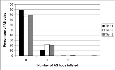
Figure 4: The path inflation percentage per tier in a synthetic graph, generated with $\alpha=0.5$ and $p=0.07$.

Fig. 3 shows the Complementary Cumulative Density Function for regional distribution ($CCDF_{R}$) of the degree distribution in the Internet’s AS-graph and in the GdTang generated synthetic networks. For the synthetic networks, each $CCDF_{R}$ curve is the average taken over the 10 randomly generated networks.

The figure shows the well-known power-law of the Internet AS graph, with a CCDF exponent of $\eta=1.17$. The figure also shows that the GeoDInEd model has a fairly accurate power-law exponent of $\eta=1.37$. Note that this is precisely the value predicted in Theorem 3.1—thus validating the estimations used in the proofs.

The data shows that, as predicted by Theorem 4.5, the model brings the number of leaves in the network to 49%, while the number of leaves in the AS-graph is 30%. Thus it seems that the GeoDInEd model produces too many leaves. Note, though, that the number of leaves in the AS-graph is slightly too low for the power-law that the degree distribution exhibits: Fig. 3 shows that the AS-graph’s CCDF has a “bump” for degree values 1–4. Thus we speculate that an additional process is taking place and affecting the frequency of low-connectivity nodes. Exploring and modeling this phenomenon is left for future work.

5.4 Path inflation effects

Gao and Wang [GW02] discuss path inflation in the Internet’s AS graph due to the so-called No-Valley routing policy. They reported that for tier-1 ISPs, 20% of paths exhibited path inflation. For tier-2 ISPs they found 55% path inflation and for tier-3 ISPs they found 20% path inflation. In order to compare these findings to the behavior on our synthetic networks, we define the No-Valley routing policy as follows:

No-Valley Routing Policy: an AS does not provide transit services between any two of its providers. That is, in an AS path ($u_{1},u_{2}....u_{n}$) if ($u_{i},u_{i+1}$) has a provider-customer relationship, then ($u_{j},u_{j+1}$) must have a provider-customer relationship for any $i<j<n$. We divided the AS-es into tiers based on node degrees in the following way :

Tier1 - nodes with $Deg(node)\geq 100$

Tier2 - nodes with $20\leq{Deg(node)}<100$

Tier3 - nodes with $3\leq{Deg(node)}<20$

We adopted the algorithm proposed by Gao and Wang [GW02] for computing the shortest AS path among all no-valley paths, using our definition of No-Valley routing policy and used it to calculate path inflation within the three tiers. Fig. 4 shows that the results we obtained are fairly close to those shown by Gao and Wang [GW02]: 11% path inflation for tier-1, 22% path inflation for tier-2, and 23% infaltion for tier-3.

6 Conclusions and Future Work

We have shown that our model, the GeoDInEd model, significantly improves upon previously suggested models. Most importantly, our model produces directed graphs, which allow a much more appropriate representation of the AS-graph’s Customer-Provider peering arrangements, as well as a representation of symmetric peer-to-peer arrangements. Besides being more realistic, GeoDInEd even improves upon earlier, undirected, models in terms of the (undirected) power-law exponent. Using a simple notion of geography, our model shows that different clustering structures can all manifest the same power-law. Moreover, in addition to the global dense core, for the first time, our model produces regional dense cores, when peering arrangements have a 50% probability of being regional. Our model also exhibits realistic path inflation effects. Finally, our model is amenable to mathematical analysis, and is implemented as a freely available network generator.

References

- [AB00] Réka Albert and Albert-László Barabási. Topology of evolving networks: Local events and universality. Physical Review Letters., 85(24):5234–5237, December 2000.
- [ACL01] W. Aiello, F. Chung, and L. Lu. Random evolution in massive graphs. In Proc. 42nd IEEE Symp. Foundations of Computer Science (FOCS), pages 510–519, 2001.
- [AJB00] R. Albert, H. Jeong, and A.-L. Barabási. Error and attack tolerance of complex networks. Nature, 406:378–382, 2000.
- [BA99] Albert-László Barabási and Réka Albert. Emergence of scaling in random networks. Science, 286:509–512, 15 October 1999.
- [BB01] G. Bianconi and A. L. Barabási. Competition and multiscaling in evolving networks. Europhysics Letters, 54(4):436–442, 2001.
- [BBCR03] B. Bollobás, C. Borgs, J. Chayes, and O. Riordan. Directed scale-free graphs. In Proc. 14th ACM-SIAM Symposium on Discrete Algorithms, pages 132–139, 2003.
- [BGW04] S. Bar, M. Gonen, and A. Wool. An incremental super-linear preferential Internet topology model. In Proc. 5th Annual Passive & Active Measurement Workshop (PAM), LNCS 3015, pages 53–62, Antibes Juan-les-Pins, France, April 2004. Springer-Verlag.
- [BRCH03] D. Ben-Avraham, A.F. Rozenfeld, R. Cohen, and S. Havlin. Geographical embedding of scale-free networks. In Randomness and Complexity, 2003.
- [BS02] R.X. Brunet and I.M. Sokolov. Evolving networks with disadvantaged long-range connections. Physical Review E, 66(026118), 2002.
- [BT02] T. Bu and D. Towsley. On distinguishing between Internet power-law generators. In Proc. IEEE INFOCOM’02, New-York, NY, USA, April 2002.
- [CAI04] IPv4 BGP geopolitical analysis. http://www.caida.org/analysis/geopolitical/bgp2country/, 2004.
- [CCG+02] Q. Chen, H. Chang, R. Govindan, S. Jamin, S. Shenker, and W. Willinger. The origin of power laws in Internet topologies revisited. In Proc. IEEE INFOCOM’02, New-York, NY, USA, April 2002.
- [CEBH00] R. Cohen, K. Erez, D. Ben-Avraham, and S. Havlin. Resilience of the Internet to random breakdowns. Physical Review Letters., 85(21):4626–4628, November 2000.
- [CGJ+02] H. Chang, R. Govindan, S. Jamin, S. Shenker, and W. Willinger. Towards capturing representative as-level Internet topologies. In Proc. ACM SIGCOMM, 2002.
- [CHK+01] D. Callaway, J. Hopcroft, J. Kleinberg, M. Newman, and S.H. Strogatz. Are randomly grown graphs really random. Physical Review Letters., 64, 2001.
- [CL02] F. Chung and L. Lu. Connected components in random graphs with given expected degree sequences. Annals of Combinatorics, 6:125–145, 2002.
- [CM04a] A. Clauset and C. Moore. Traceroute sampling makes random graphs appear to have power law degree distributions. 2004. Preprint, Submitted to Physical Review Letters.
- [CM04b] A. Clauset and C. Moore. Why mapping the Internet is hard, 2004. arXiv:cond-mat/0407339.
- [DJMS03] D. Dolev, S. Jamin, O. Mokryn, and Y. Shavitt. Internet resiliency to attacks and failures under bgp policy routing. Technical Report 2003-79, Dept. Computer Science, The Hebrew University, 2003. Available from http://www.eng.tau.ac.il/~osnaty.
- [DMS01] S.N. Dorogovtsev, J.F.F. Mendes, and A.N. Samukhin. Giant strongly connected component of directed networks. Physical Review E, 64, 2001.
- [ER60] P. Erdős and A. Renyi. On the evolution of random graphs. Magyar Tud. Akad. Mat. Kutato Int. Kozl., 5:17–61, 1960.
- [FKP01] U. Feige, G. Kortsarz, and D. Peleg. The dense k-subgraph problem. Algorithmica, 29(3):410–421, 2001.
- [Gao01] L. Gao. On inferring automonous system relationships in the Internet. IEEE/ACM Trans. on Networking, 9:733–745, 2001.
- [GK03] S.P. Gorman and R. Kulkarni. Spatial small worlds: New geographic patterns for information economy, 2003. arXiv:cond-mat/0310426.
- [GMZ03] C. Gkantsidis, M. Mihail, and E. Zegura. Spectral analysis of Internet topologies. In Proc. IEEE INFOCOM’03, New-York, NY, USA, April 2003.
- [GW02] L. Gao and F. Wang. The extent of AS path inflation by routing policies. In Proc. IEEE Global Internet Symposium, 2002.
- [JJ02] J. Jost and M.P. Joy. Evoloving networks with distance preferences. Physical Review E, 66(036126), 2002.
- [KRR01] P.L. Krapivsky, G.J. Rodgers, and S. Render. Degree distributions of growing networks. Physical Review Letters, 86:5401, 2001.
- [LBCM03] A. Lakhina, J.W. Byers, M. Crovella, and I. Matta. On the geographic location of Internet resources. IEEE Journal on Selected Areas in Communications, 21:934–948, 2003.
- [LBCX03] A. Lakhina, J. W. Byers, M. Crovella, and P. Xie. Sampling biases in IP topology measurments. In Proc. IEEE INFOCOM’03, 2003.
- [LC03] X. Li and G. Chen. A local-world evolving network model. Physica A, 328:274–286, 2003.
- [LPS04] H. Lee, A. Perrig, and D. Smith. BASE: An incrementally deployable mechanism for viable IP spoofing prevention. Manuscript, 2004.
- [MLMB01] A. Medina, A. Lakhina, I. Matta, and J. Byers. BRITE: An approach to universal topology generation. In Proceedings of MASCOTS’01, August 2001.
- [MR95] M. Molloy and B. Reed. A critical point for random graphs with a given degree sequence. Structures and Algorithms, 6:161–180, 1995.
- [NSW01] M.E.J. Newman, S.H. Strogatz, and D.J. Watts. Random graphs with arbitrary degree distributions and their applications. Physical Review Letters., 64, 2001.
- [PR04] T. Petermann and P. De Los Rios. Exploration of scale-free networks - do we measure the real exponents? Europhysics Letters, 38:201–204, 2004.
- [RN04] H. Reittu and I. Norros. On the power law random graph model of the Internet. Performance Evaluation, 55, January 2004.
- [SARK02] L. Subramanian, S. Agarwal, J. Rexford, and R. H. Katz. Characterizing the Internet hierarchy from multiple vantage points. In Proc. IEEE INFOCOM’02, New-York, NY, USA, April 2002.
- [SFFF03] G. Siganos, M. Faloutsos, P. Faloutsos, and C. Faloutsos. Power-laws and the AS-level Internet topology. IEEE/ACM Trans. on Networking, 11:514–524, 2003.
- [SW03] G. Sagie and A. Wool. A clustering-based comparison of Internet topology models, 2003. Preprint.
- [SW04] G. Sagie and A. Wool. A clustering approach for exploring the Internet structure. In Proc. 23rd IEEE Convention of Electrical & Electronics Engineers in Israel (IEEEI), September 2004.
- [TGJ+02] H. Tangmunarunkit, R. Govindan, S. Jamin, S. Shenker, and W. Willinger. Network topology generators: Degree based vs. structural. In Proc. ACM SIGCOMM, 2002.
- [TPSF01] L. Tauro, C. Palmer, G. Siganos, and M. Faloutsos. A simple conceptual model for Internet topology. In IEEE Global Internet, San Antonio, TX, November 2001.
- [WGJ+02] W. Willinger, R. Govindan, S. Jamin, V. Paxson, and S. Shenker. Scaling phenomena in the internet: Critically examining criticality. Proceedings of the National Academy of Sciences of the United States of America, 99:2573–2580, February 2002.
- [WJ02] Jared Winick and Sugih Jamin. Inet-3.0: Internet topology generator. Technical Report UM-CSE-TR-456-02, Department of EECS, University of Michigan, 2002.
- [WLC04] J. Wang, X. Liu, and A. A. Chien. Empirical study of tolerating denial-of-service attacks with a proxy network. Manuscript, 2004.
- [WSS02] C.P. Warren, L.M. Sander, and I.M. Sokolov. Geography in a scale-free network model. Physical Review E, 66(056105), 2002.
- [ZM04] S. Zhou and R. J. Mondragon. The rich-club phenomenon in the Internet topology. IEEE Communications Letters, 8(3), March 2004.