Unified Large System Analysis of MMSE and Adaptive Least Squares Receivers for a class of Random Matrix Channels

Abstract

We present a unified large system analysis of linear receivers for a class of random matrix channels. The technique unifies the analysis of both the minimum-mean-squared-error (MMSE) receiver and the adaptive least-squares (ALS) receiver, and also uses a common approach for both random i.i.d. and random orthogonal precoding. We derive expressions for the asymptotic signal-to-interference-plus-noise (SINR) of the MMSE receiver, and both the transient and steady-state SINR of the ALS receiver, trained using either i.i.d. data sequences or orthogonal training sequences. The results are in terms of key system parameters, and allow for arbitrary distributions of the power of each of the data streams and the eigenvalues of the channel correlation matrix. In the case of the ALS receiver, we allow a diagonal loading constant and an arbitrary data windowing function. For i.i.d. training sequences and no diagonal loading, we give a fundamental relationship between the transient/steady-state SINR of the ALS and the MMSE receivers. We demonstrate that for a particular ratio of receive to transmit dimensions and window shape, all channels which have the same MMSE SINR have an identical transient ALS SINR response. We demonstrate several applications of the results, including an optimization of information throughput with respect to training sequence length in coded block transmission.

I Introduction

Large-system analysis of linear receivers for random matrix channels has attracted significant attention in recent years, and has proven to be a powerful tool in their understanding and design (e.g., see [1] and references therein). In particular, large-system analysis of the matched filter, decorrelator, and minimum-mean-squared-error (MMSE) receivers, which have knowledge of the channel state information, has been exhaustively studied for the downlink, using results such as the Silverstein-Bai theorem [2], Girko’s law [3], and free probability [4]. In this paper we take a different approach to the problem, which allows us to consider random i.i.d. and orthogonal channels (or matrix of signatures) in the same treatment, in contrast to the existing separate analyses of i.i.d. [5] and orthogonal [6, 7] channels. The new approach also allows us to consider a more general class of signal models, and a receiver which does not have the benefit of channel state information, namely the adaptive least-squares (ALS) receiver.

In this paper, we consider both the MMSE and ALS receivers. The ALS receiver approximates the MMSE receiver and requires training symbols [8]. In particular, the autocorrelation matrix of the received vector (an ensemble average), which is used in the MMSE receiver, is replaced in the ALS receiver by a sample autocorrelation matrix (a time average). Given sufficient training symbols, the performance of the ALS receiver approaches that of the MMSE receiver. In this paper, two types of adaptive training modes are considered, based on those presented in [9], where either the training sequence is known at the receiver, or a semi-blind method is employed. In a time-varying environment, weighting can be applied to the errors to create data windowing, which allows for tracking. When implemented online as a series of rank-1 updates with exponential windowing, this receiver is often referred to as the recursive least-squares (RLS) receiver [8]. To prevent ill-conditioning of the sample autocorrelation matrix with RLS filtering, diagonal loading can be employed, which refers to initializing this matrix with a small positive constant times the identity matrix.

Prior relevant work on ALS techniques (in particular, as applied to channel equalization and estimation) includes [10], where an approximate expression is derived for the transient excess mean-squared-error (MSE) of the ALS receiver with respect to the MMSE receiver, often referred to as self-noise, for a general channel model and windowing function. Also, an approximate expression is given for the convergence time constant of the receiver when tracking non-stationary signals. Steady-state and transient analysis of the RLS receiver was also considered in [11]. A comprehensive treatment of ALS techniques and variations is contained in [8].

The application of ALS to CDMA was considered in [12], where the convergence of a blind multiuser detector based on a stochastic gradient-descent adaptation rule is also analyzed. In [9], approximate expressions are given for the relationship between the MMSE signal-to-interference-plus-noise-ratio (SINR) and the steady-state ALS SINR with exponential windowing for DS-CDMA in flat-fading. This was extended in [13] to a steady-state analysis of two-stage algorithms based on RLS using decision-directed adaptation. A review of adaptive interference mitigation techniques is given in [14].

Large-system analysis for ALS receivers was first considered in [15, 16], which considered DS-CDMA in flat fading with i.i.d. training sequences, and an ALS receiver with diagonal loading and rectangular or exponential weighting. The transient SINR (i.e., after a given number of training symbols) and steady-state SINR (i.e., after an unlimited number of training symbols) of the ALS receiver was derived in the limit where the number of transmit dimensions, the number of multiplexed data streams, and the number of training symbols all tend to infinity with fixed ratios. With rectangular windowing and no diagonal loading, a relationship between the MMSE SINR and the transient ALS SINR was given. In other work, large-system analysis has been applied to so-called subspace-based blind ALS receivers in [17, 18, 19].

In this paper, we consider a more general complex-valued AWGN matrix-vector channel model of the form ${\mathbf{r}}={\mathbf{H}}{\mathbf{S}}{\mathbf{A}}{\mathbf{b}}+{\mathbf{n}}$, where ${\mathbf{H}}$ is an arbitrary matrix, ${\mathbf{A}}$ is an arbitrary diagonal matrix, and ${\mathbf{S}}$ is either an i.i.d. or orthogonal matrix. For example, the model applies explicitly to downlink synchronous direct sequence (DS) or multi-carrier (MC) CDMA in frequency-selective fading, as well as multi-input multi-output (MIMO) channels. In fact, if we additionally require that the data vector ${\mathbf{b}}$ is unitarily invariant, then the MMSE and ALS results we obtain apply to all AWGN matrix-vector systems of the form ${\mathbf{r}}={\mathbf{C}}{\mathbf{b}}+{\mathbf{n}}$, provided that the eigenvalues of ${\mathbf{C}}{\mathbf{C}}^{\dagger}$ converge to a well-behaved deterministic distribution. As such, the results can be applied to systems not previously considered in large-system analysis, such as equalization of single-user finite-impulse-response (FIR) channels.

For this channel model, we derive the SINR of the MMSE receiver, with either i.i.d. or orthogonal ${\mathbf{S}}$, in the large-system limit where the number of transmit and receive dimensions, and the number of multiplexed data streams all tend to infinity with fixed ratios. The expression for the SINR is a function of these ratios and the received SNR, and allows for arbitrary asymptotic eigenvalue distributions (a.e.d.’s) of ${\mathbf{A}}{\mathbf{A}}^{\dagger}$ and ${\mathbf{H}}{\mathbf{H}}^{\dagger}$. This result can also be derived under the same set of assumptions using the S-transform from free probability. However, unlike the free probability technique, we show that the technique used to derive this result also applies to the ALS receiver.

For the ALS receiver, we extend the work of [16] to the general channel model described. We consider an arbitrary data windowing function and both i.i.d. and orthogonal training sequences. That is, we determine both the transient and steady-state ALS SINR in the limit described for the MMSE receiver, and also as the number of training symbols tend to infinity.

Also, we present an expression which relates the SINR of the MMSE receiver to the transient and steady-state SINRs of the ALS receiver for the case of i.i.d. training sequences and no diagonal loading. We demonstrate that in this situation, for a particular ratio of receive to transmit dimensions and window shape, all channels, which have the same MMSE SINR, have an identical transient ALS SINR response. Since our results hold for all well-behaved matrix-vector systems for which the data vector is unitarily invariant (as previously discussed), the MMSE-ALS relationship is in fact seen to be a fundamental property of adaptive least-squares estimation.

It is interesting to compare our results to an approximate expression for the steady-state ALS SINR given in [9] for the special case of DS-CDMA in a flat-fading channel, with i.i.d. spreading and exponential weighting. A comparison of the expressions reveals the approximation in [9] to be excellent, particularly for large window sizes. Also, we note that for a general channel model, the study in [11] previously came to the conclusion that the ALS convergence rate is independent of the channel; however, their conclusion was based on making several approximations, and only exponential windowing (RLS) was considered. This conclusion was stated for DS-CDMA in [9]; however, an explicit relationship between the MMSE SINR and the transient ALS SINR, such as derived in this paper, is not given in either of those papers.

Unfortunately, we have not determined a simple relationship between the MMSE SINR and ALS SINR with orthogonal training sequences and/or diagonal loading. This remains an open problem. Inspection reveals that with orthogonal training sequences and no diagonal loading, the transient relationship will depend on the channel.

During the course of the analysis we solve for the Stieltjés (or Cauchy) transforms of the a.e.d.’s of both the autocorrelation matrix and the weighted sample autocorrelation matrix of the received signal. These expressions are found using matrix manipulations, which do not require the use of free probability. The first transform can also be derived using free probability; however, such techniques cannot be applied to derive the second transform, since the associated constituent matrices are not free. As such, the results are of independent mathematical interest.

Through numerical studies, we demonstrate the applicability of the large-system results to finite systems, and the benefits of orthogonal precoding and training is examined. We demonstrate an application of the results in the optimization of information throughput with respect to training sequence length in coded block transmission.

The paper is arranged as follows. Section II outlines the general transmission model, the receivers considered, and defines the large-system asymptotic limit. Section III discusses the general approach we take for the analysis. Section IV reviews analytical approaches to the MMSE SINR problem, and presents the general solution based on the unified analytical approach. An alternate expression for the MMSE SINR, different from those presented in [1], is also presented which allows the relationship between the MMSE SINR and ALS SINR to be derived in certain cases in later sections. Section V presents the general result for the ALS SINR. A simple relationship between the ALS SINR and MMSE SINR with i.i.d. training and without diagonal loading is then presented in Section VI. Finally, numerical studies are presented in Section VII.

II System Model

This paper considers a general matrix-vector transmission model. It applies to a wide range of practical data communication systems, including frequency-flat fading MIMO channels, and both frequency-flat and frequency-selective fading downlink DS- or MC-CDMA channels.

II-A General Transmission Model

In matrix notation, the received signal in the $m^{\text{th}}$ symbol period is

$${\mathbf{r}}_{m}={\mathbf{H}}{\mathbf{S}}{\mathbf{A}}{\mathbf{b}}_{m}+{\mathbf{n}}_{m}$$ (1)

where

• ${\mathbf{H}}$ is an $M\times N$ complex-valued channel matrix.

• ${\mathbf{S}}=\left[{\mathbf{s}}_{1}\cdots{\mathbf{s}}_{K}\right]$ is an $N\times K$ complex-valued matrix which contains either

  • random orthonormal columns, i.e., we assume that ${\mathbf{S}}$ is obtained by extracting $K\leq N$ columns from an $N\times N$ Haar-distributed unitary random matrix, or,

  • i.i.d. complex elements with mean zero and variance $\frac{1}{N}$. For example, i.i.d. real & imaginary parts which are either $\pm 1/\sqrt{2N}$ with equal probability, or i.i.d. Gaussian with zero mean and variance $1/(2N)$.

  We shall call the first case ‘isometric ${\mathbf{S}}$’, and the second case ‘i.i.d. ${\mathbf{S}}$’, as is done in [6].

• ${\mathbf{A}}$ is a $K\times K$, diagonal, complex-valued matrix of transmit coefficients, i.e. ${\mathbf{A}}=\operatorname{diag}(A_{1},\ldots,A_{K})$. In fact, the results which follow depend only the values of $P_{k}=|A_{k}|^{2}$, and so to simplify notation, without lack of generality, we may assume $A_{k}$, $k=1,\ldots,K$, is non-negative and real valued.

• The complex vector ${\mathbf{b}}_{m}$ is $K\times 1$ and either contains transmit data, or training symbols (for an ALS receiver). Elements of ${\mathbf{b}}_{m}$ can be either i.i.d. with zero mean and unit variance (for data and i.i.d. training cases), or they can be drawn from a set of orthogonal sequences (for orthogonal training, as explained further in Section II-D).

• ${\mathbf{n}}_{m}$ contains i.i.d., zero mean, circularly symmetric, complex Gaussian entries with variance per dimension $\sigma^{2}/2$.

• ${\mathbf{H}}$, ${\mathbf{S}}$, ${\mathbf{A}}$, ${\mathbf{b}}_{m}$, and ${\mathbf{n}}_{m}$ are mutually independent.

II-B Discussion

The general transmission model in (1) is widely applicable, and in particular includes the following systems.

• Downlink MC- or DS-CDMA: In this case, ${\mathbf{S}}$ represents the matrix of $K$ signatures with spreading gain $N$. Typically, the number of output dimensions equals the number of input dimensions and hence ${\mathbf{H}}$ is square.

  • For flat-fading DS-CDMA, ${\mathbf{H}}={\mathbf{I}}_{N}$ and ${\mathbf{A}}$ represents the combined effect of each users’ transmit power and channel coefficient.

  • For MC-CDMA in frequency-selective fading, ${\mathbf{H}}$ is the diagonal matrix of the channel frequency response in each subcarrier, and ${\mathbf{A}}$ represents the transmit amplitude of each signature.

  • For DS-CDMA in frequency-selective fading, ${\mathbf{H}}$ is a circulant or Toeplitz matrix constructed from the channel impulse response, and ${\mathbf{A}}$ represents the transmit amplitude of each signature.

• ‘Rich’ MIMO: The standard point-to-point flat fading MIMO channel model is given by (1), where $K$ and $N$ correspond to the number of transmit and receive antennas, respectively. The standard MIMO channel matrix with i.i.d. circularly symmetric complex Gaussian coefficients between each pair of transmit and receive antennas corresponds here to setting ${\mathbf{H}}={\mathbf{I}}_{N}$ and ${\mathbf{S}}$ i.i.d. Gaussian. The matrix ${\mathbf{A}}$ defines the transmit amplitudes on each antenna.

• MIMO with richness parameter: The MIMO channel model introduced in [20] can also be described by (1), with ${\mathbf{S}}$ i.i.d. and ${\mathbf{H}}={\boldsymbol{\Phi}}{\mathbf{C}}$, where ${\boldsymbol{\Phi}}$ is i.i.d., and ${\mathbf{C}}$ is diagonal. In this case, ${\mathbf{S}}$ models the propagation from the transmitter to a ‘scattering array’, modeled by ${\mathbf{C}}$, and ${\boldsymbol{\Phi}}$ models the propagation from the scattering array to the receiver. The rank of the scattering array matrix determines the richness of the MIMO channel.

• If we additionally require that the data vector ${\mathbf{b}}$ is unitarily invariant, then the MMSE and ALS asymptotic SINR results we obtain apply to all AWGN matrix-vector systems of the form ${\mathbf{r}}={\mathbf{C}}{\mathbf{b}}+{\mathbf{n}}$, under certain conditions on the channel matrix ${\mathbf{C}}$, and the data and noise vectors, ${\mathbf{b}}$ and ${\mathbf{n}}$. A full explanation is given in Section II-E.

II-C MMSE Receiver

The output of the MMSE receiver with full channel state information (CSI) and knowledge of ${\mathbf{S}}$ for stream $k$ at symbol interval $m$ is given by

$$\hat{{\mathbf{b}}}_{m}(k)={\mathbf{c}}_{k}^{\dagger}{\mathbf{r}}_{m}$$ (2)

where

$${\mathbf{c}}_{k} ={\mathbf{R}}^{-1}{\mathbf{H}}{\mathbf{s}}_{k}$$ (3)

$${\mathbf{R}} =({\mathbf{H}}{\mathbf{S}}{\mathbf{A}})^{\ddagger}+\sigma^{2}{\mathbf{I}}_{M}$$ (4)

Now, identifying the signal and interference components of the received signal in (1), i.e., ${\mathbf{r}}_{m}=A_{k}{\mathbf{H}}{\mathbf{s}}_{k}{\mathbf{b}}_{m}(k)+{\mathbf{r}}_{m}^{I}$, the corresponding output SINR is defined as

$$\text{SINR}^{\text{MMSE}}_{k,N} =\frac{\textsf{{E}}[|{\mathbf{c}}_{k}^{\dagger}({\mathbf{r}}_{m}-{\mathbf{r}}_{m}^{I})|^{2}]}{\textsf{{E}}[|{\mathbf{c}}_{k}^{\dagger}{\mathbf{r}}_{m}^{I}|^{2}]}$$ (5)

where the expectation in (5) is with respect to ${\mathbf{b}}_{m}$ and ${\mathbf{n}}_{m}$. The subscript $N$ indicates that this is a non-asymptotic quantity.

II-D ALS Receiver

The output of the adaptive least-squares (ALS) receiver with $i$ training symbols for stream $k$ at symbol interval $m>i$ is given by

$$\hat{{\mathbf{b}}}_{m}(k) =\hat{{\mathbf{c}}}_{k}^{\dagger}{\mathbf{r}}_{m}$$ (6)

where

$$\hat{{\mathbf{c}}}_{k} =\hat{{\mathbf{R}}}^{-1}\hat{{\mathbf{s}}}_{k}$$ (7)

$$\hat{{\mathbf{R}}} =\frac{1}{i}\mathcal{R}{\mathbf{W}}\mathcal{R}^{\dagger}+\frac{\mu}{\eta}{\mathbf{I}}_{M}$$ (8)

$$\mathcal{R} ={\mathbf{H}}{\mathbf{S}}{\mathbf{A}}{\mathbf{B}}^{\dagger}+{\mathbf{N}}$$ (9)

$$\hat{{\mathbf{s}}}_{k} =\begin{cases}\frac{1}{i}\mathcal{R}{\mathbf{W}}\underline{{\mathbf{b}}}_{k}&\text{, with training}\\ {\mathbf{H}}{\mathbf{s}}_{k}&\text{, semi-blind}\end{cases}$$ (10)

and where

• ${\mathbf{B}}$ is an $i\times K$ matrix of training data, where the $m^{\text{th}}$ row of ${\mathbf{B}}$ is ${\mathbf{b}}_{m}^{\dagger}$. The $k^{\text{th}}$ column of ${\mathbf{B}}$ will be denoted as $\underline{{\mathbf{b}}}_{k}$. We consider both i.i.d. and orthogonal training sequences, i.e.,

  • ${\mathbf{B}}$ contains i.i.d. elements with zero mean, unit variance, and finite positive moments, or,

  • ${\mathbf{B}}$ contains either random orthogonal rows or columns. If $K<i$ then ${\mathbf{B}}^{\dagger}{\mathbf{B}}=i{\mathbf{I}}_{K}$, and we assume that $\frac{1}{\sqrt{i}}{\mathbf{B}}$ is obtained by extracting $K$ columns from an $i\times i$ Haar-distributed unitary random matrix. If $K>i$, then ${\mathbf{B}}{\mathbf{B}}^{\dagger}=K{\mathbf{I}}_{i}$, and we assume that $\frac{1}{\sqrt{K}}{\mathbf{B}}^{\dagger}$ is obtained by extracting $i$ columns from a $K\times K$ Haar-distributed unitary random matrix.

• ${\mathbf{N}}$ is an $M\times i$ matrix of noise, where the $m^{\text{th}}$ column is ${\mathbf{n}}_{m}$.

• $\mu$ is a real-valued non-negative diagonal loading constant, i.e., $\mu\in{\Bbb{R}}^{*}$, and $\eta=i/N$.

• ${\mathbf{W}}$ is an $i\times i$ diagonal real-valued data windowing matrix, i.e. ${\mathbf{W}}=\operatorname{diag}(w_{1},\ldots,w_{i})$ where $w_{m}\in{\Bbb{R}}^{*}$ for $m=1,\ldots,i$. For example, with exponential weighting $w_{m}=\epsilon^{i-m}$, where $\epsilon\in(0,1]$, or, without data windowing ${\mathbf{W}}={\mathbf{I}}_{i}$.

Note that, although strictly speaking the model in (1) applies only to time-invariant systems, we include windowing to allow for practical situations such as slowly time varying channels, or users entering/leaving the system. The term ‘semi-blind’ in (10) refers to the case when ${\mathbf{H}}$ and ${\mathbf{s}}_{k}$ are known, and there is no training data, whereas ‘with training’ refers to when just ${\mathbf{B}}$ is known. For more details on the practical issues, see [9], where this ALS formulation is considered for DS-CDMA in flat-fading.

The SINR for the $k^{\text{th}}$ stream at the output of the ALS receiver, $\text{SINR}^{\text{ALS}}_{k,N}$, is defined by the right-hand side of (5), however, with ${\mathbf{c}}_{k}$ replaced by $\hat{{\mathbf{c}}}_{k}$.

II-E Large System Limit

We define $\alpha=K/N$ and $\beta=M/N$, and for the ALS receiver, $\eta=i/N$.

Throughout this paper we consider the asymptotic limit $(M,N,K,i)\to\infty$ with $K/N\to\alpha>0$, $i/N\to\eta>0$, and $M/N\to\beta>0$ constant.

With data windowing it is necessary to consider how ${\mathbf{W}}$ is defined for each $i$ so that the empirical distribution function (e.d.f.) of its diagonal values converges to something appropriate. Any finite window length becomes negligible in the large system limit as $i\to\infty$, therefore it is necessary to scale the window shape with the system size. For example, as in [16], with exponential windowing we define $L=\frac{1}{1-\epsilon}$ as the ‘average’ window length, and take $L\to\infty$ with $L/N\to\bar{L}>0$ constant.

To facilitate the large system analysis, we also require that ${\mathbf{H}}^{\ddagger}$, ${\mathbf{A}}^{2}$, and ${\mathbf{W}}$ each have a uniformly bounded spectral norm, that is, a bound which is independent of the system dimension $N$. Also, we require the empirical distribution functions of the eigenvalues of ${\mathbf{A}}^{2}$, ${\mathbf{H}}^{\ddagger}$, and ${\mathbf{W}}$ to converge in distribution almost surely to non-random distributions on the non-negative real axis, which will have compact support due to the previous assumption. We also assume that the limiting distributions of ${\mathbf{A}}^{2}$, ${\mathbf{H}}^{\ddagger}$, and ${\mathbf{W}}$ are non-trivial, i.e., do not have all mass at zero.

Proposition 1

The large-system MMSE and ALS SINRs corresponding to the transmission model in (1) are the same as the large-system MMSE and ALS SINRs, respectively, computed for any matrix-vector system of the form ${\mathbf{r}}={\mathbf{C}}{\mathbf{b}}+{\mathbf{n}}$ in which

• ${\mathbf{C}}$, ${\mathbf{b}}$, and ${\mathbf{n}}$ are mutually independent,

• the $M\times 1$ noise vector ${\mathbf{n}}$ satisfies the same conditions as ${\mathbf{n}}_{m}$ above,

• the $K\times 1$ data/training vector ${\mathbf{b}}$ satisfies the same conditions as ${\mathbf{b}}_{m}$ above, and additionally is unitarily invariant,

• the $M\times K$ channel matrix ${\mathbf{C}}$ is such that the e.d.f. of ${\mathbf{C}}^{\ddagger}$ satisfies the conditions on ${\mathbf{H}}^{\ddagger}$ mentioned in the previous paragraph,

and corresponds to taking ${\mathbf{H}}={\mathbf{C}}$, ${\mathbf{S}}$ to be $K\times K$ isometric, and ${\mathbf{A}}={\mathbf{I}}_{K}$, respectively.

Proof:

Since ${\mathbf{b}}$ is unitarily invariant, all data streams have identically distributed SINRs. Since ${\mathbf{b}}$ has the same distribution as ${\mathbf{U}}{\mathbf{b}}$, where ${\mathbf{U}}$ is a $K\times K$ Haar-distributed random unitary matrix, we see that the distribution of the MMSE and ALS SINR associated with ${\mathbf{r}}^{\prime}={\mathbf{C}}{\mathbf{U}}{\mathbf{b}}+{\mathbf{n}}$ are, respectively, the same as that for ${\mathbf{r}}$, and will share a common large-system limit, if it exists.         

Proposition 1 implies that our model encompasses the classic equalization model. Namely, ${\mathbf{r}}$ represents $N=M$ samples at the output of a single-input/single-output (SISO) FIR channel ${\mathbf{h}}$ of length $L_{c}$, i.e., ${\mathbf{r}}(n)=\sum_{\ell=0}^{L_{c}-1}{\mathbf{h}}(\ell){\mathbf{b}}(n-\ell)+{\mathbf{n}}(n)$. If a cyclic prefix of appropriate length is used, we set ${\mathbf{C}}$ defined in Proposition 1 equal to the circulant channel matrix. Therefore, from Proposition 1, the corresponding model (1) takes ${\mathbf{A}}={\mathbf{I}}_{N}$, ${\mathbf{S}}$ as $N\times N$ isometric, and ${\mathbf{H}}$ as ${\mathbf{C}}$ or equivalently as an $N\times N$ diagonal matrix with the $N$-point DFT of ${\mathbf{h}}$ on the diagonal.

III Unified Large System Analysis

In Sections IV and V, we derive the asymptotic SINR for the model (1) with both MMSE and ALS receivers. The SINR in both cases is directly related to the Stieltjés transform of the a.e.d. of the received signal correlation matrix ${\mathbf{R}}$ for the MMSE receiver, and $\hat{{\mathbf{R}}}$ for the ALS receiver. For the MMSE case, there are a number of existing methods for finding such transforms directly (see e.g., [1]). However, those methods do not extend to the ALS problem. We now discuss a general approach, which applies to both i.i.d. and isometric ${\mathbf{S}}$ for both the MMSE and the ALS receiver.

The aim is to derive a set of equations for each “constituent” dimension in ${\mathbf{R}}$ (or $\hat{{\mathbf{R}}}$), which can be solved for the Stieltjés transform. For example, ${\mathbf{R}}$ has three constituent dimensions ($K$, $N$, and $M$), while $\hat{{\mathbf{R}}}$ has four, since it also includes $i$.

Each equation is based on expanding the simple identity ${\mathbf{R}}^{-1}{\mathbf{R}}={\mathbf{I}}_{M}$ (or $\hat{{\mathbf{R}}}^{-1}\hat{{\mathbf{R}}}={\mathbf{I}}_{M}$) in each constituent dimension. That is, since ${\mathbf{R}}$ (or $\hat{{\mathbf{R}}}$) is Hermitian, this term in the identity can be written as a sum of vector outer products, where the sum index runs up to the value of the dimension. Taking the normalized trace of both sides of the resulting equation can be simplified, and involves terms which have equivalent asymptotic forms, which can be evaluated using an asymptotic extension to the matrix inversion lemma. These equivalent forms are in terms of scalar variables, some of which are mixed matrix moments. Each of these moments can be expressed in terms of the other variables.

The result is a set of equations, which can be solved for the Stieltjés transform, and other unknowns (e.g., various matrix moments). Interestingly, in all cases we consider, the equations can be written in a form such that solving for the Stieltjés transform numerically amounts to zero-finding in at most two dimensions.

IV Analysis of MMSE Receiver

It has been shown that, for both i.i.d. and isometric ${\mathbf{S}}$, the asymptotic SINR for the $k^{\text{th}}$ stream at the output of the full-CSI MMSE receiver in (3) satisfies [21, 7]

$$\max_{k\leq K}\left|{\text{SINR}^{\text{MMSE}}_{k,N}-P_{k}\rho_{1}^{N}}\right| \stackrel{{\scriptstyle a.s.}}{{\longrightarrow}}0$$ (11)

under the limit considered, where $\stackrel{{\scriptstyle a.s.}}{{\longrightarrow}}$ denotes almost-sure convergence,

$$\rho_{1}^{N} =\begin{cases}\frac{1}{N}\mathrm{tr}[{\mathbf{H}}^{\dagger}{\mathbf{R}}^{-1}{\mathbf{H}}]&\text{, i.i.d.\@ ${\mathbf{S}}$,}\\ \frac{1}{N-K}\mathrm{tr}[{\boldsymbol{\Pi}}{\mathbf{H}}^{\dagger}{\mathbf{R}}^{-1}{\mathbf{H}}]&\text{, iso.\ ${\mathbf{S}}$},\end{cases}$$ (12)

and ${\boldsymbol{\Pi}}={\mathbf{I}}_{N}-{\mathbf{S}}^{\ddagger}$.

We now discuss some existing methods for computing the limit of the moment $\rho_{1}^{N}$ in (12) with the MMSE full-CSI receiver, and note that the methods do not extend to the ALS receiver. We then present the main result of this section, namely, a general SINR expression, which applies to both i.i.d. and isometric ${\mathbf{S}}$, derived using the approach discussed in Section III.

For i.i.d. ${\mathbf{S}}$, and square invertible ${\mathbf{H}}$, the SINR can be obtained in terms of the limiting distribution of ${\mathbf{H}}^{\ddagger}$ and ${\mathbf{A}}^{2}$, using the result of Silverstein and Bai [2] after writing

$$\rho_{1}^{N} =\frac{1}{N}\mathrm{tr}[({\mathbf{S}}{\mathbf{A}}^{2}{\mathbf{S}}^{\dagger}+\sigma^{2}({\mathbf{H}}^{\dagger}{\mathbf{H}})^{-1})^{-1}]$$ (13)

as was done in [22], and for more general channel distributions in [6, Theorem 2]. More generally, a solution for arbitrary (non-square) channel models can be obtained for i.i.d. ${\mathbf{S}}$ via Girko’s law (see e.g., [5, Lemma 1], or [23, Theorem IV.2] for just the Stieltjés transform of ${\mathbf{R}}$), again in terms of the limiting distributions of ${\mathbf{H}}^{\ddagger}$ and ${\mathbf{A}}^{2}$. We note that neither of these techniques can be used to compute the output SINR for the MMSE receiver with isometric ${\mathbf{S}}$, or the ALS receiver.

For isometric ${\mathbf{S}}$ and square ${\mathbf{H}}$, the asymptotic SINR was first presented in [6] with ${\mathbf{A}}={\mathbf{I}}_{K}$, and was extended in [7] to include general ${\mathbf{A}}$. Although this approach could also be used to consider non-square ${\mathbf{H}}$, it does not extend to the ALS receiver since it relies on the particular structure of ${\mathbf{R}}$, which is not shared by $\hat{{\mathbf{R}}}$.

IV-A Asymptotic SINR for MMSE Receiver

The following theorem allows us to evaluate the limit of $\rho_{1}^{N}$ (and hence the asymptotic MMSE SINR) for general channels and for either i.i.d. or isometric ${\mathbf{S}}$. The theorem is in terms of the Stieltjés transform of the e.d.f. of the eigenvalues of $({\mathbf{H}}{\mathbf{S}}{\mathbf{A}})^{\ddagger}$. That is, we generalize the definition of ${\mathbf{R}}$ from (4) by replacing $\sigma^{2}$ by a complex variable $z\in{\Bbb{C}}^{+}$ (i.e., ${\mathbf{R}}=({\mathbf{H}}{\mathbf{S}}{\mathbf{A}})^{\ddagger}-z{\mathbf{I}}_{M}$), such that the Stieltjés transform of the e.d.f. of the eigenvalues of $({\mathbf{H}}{\mathbf{S}}{\mathbf{A}})^{\ddagger}$ is given by $G_{\text{R}}^{N}(z)=\frac{1}{M}\mathrm{tr}[{\mathbf{R}}^{-1}]$. The theorem is given in terms of the two additional random variables $\rho_{1}^{N}\in{\Bbb{C}}^{+}$, as defined in (12) using the redefinition of ${\mathbf{R}}$, and $\tau_{1}^{N}\in{\Bbb{C}}^{+}$. The variable $\tau_{1}^{N}$ is defined in terms of matrix equations, and is given in Appendix B-A since the definition is lengthy and is not needed to state the following result.

Theorem 1

Under the assumptions in Section II-E, as $(M,N,K)\to\infty$ with $M/N\to\beta>0$ and $K/N\to\alpha>0$ fixed, the Stieltjés transform of the e.d.f. of the eigenvalues of $({\mathbf{H}}{\mathbf{S}}{\mathbf{A}})^{\ddagger}$, $G_{\text{R}}^{N}(z)$, $z\in{\Bbb{C}}^{+}$, along with $\rho_{1}^{N}$ and $\tau_{1}^{N}$ satisfy

$$\left|{G_{\text{R}}^{N}(z)-\gamma_{1}}\right|\stackrel{{\scriptstyle a.s.}}{{\longrightarrow}}0,$$ (14)

$$\left|{\rho_{1}^{N}-\rho_{1}}\right|\stackrel{{\scriptstyle a.s.}}{{\longrightarrow}}0,$$ (15)

$$\left|{\tau_{1}^{N}-\tau_{1}}\right|\stackrel{{\scriptstyle a.s.}}{{\longrightarrow}}0,$$ (16)

where $\gamma_{1},\rho_{1},\tau_{1}\in{\Bbb{C}}^{+}$ are solutions to

$$\gamma_{1} =-\frac{1}{z}\left(1-\frac{\alpha}{\beta}\rho_{1}\mathcal{E}_{1,1}\right)$$ (17)

$$\rho_{1} =\begin{cases}\displaystyle-z^{-1}\beta^{*}\mathcal{H}_{1,1}&\text{, i.i.d.\@ ${\mathbf{S}}$,}\\ \displaystyle\frac{-z^{-1}\beta^{*}\mathcal{H}_{1,1}}{1-\beta(1+z\gamma_{1})}&\text{, iso.\ ${\mathbf{S}}$},\end{cases}$$ (18)

$$\tau_{1} =\alpha\bar{p}-\begin{cases}\displaystyle\alpha\mathcal{E}_{1,1}&\text{, i.i.d.\@ ${\mathbf{S}}$,}\\ \displaystyle\frac{\alpha\mathcal{E}_{1,1}}{1-\beta(1+z\gamma_{1})}&\text{, iso.\ ${\mathbf{S}}$},\end{cases}$$ (19)

where $\beta^{*}=\min(\beta,1)$, and

$$\mathcal{E}_{m,1} =\textsf{{E}}\left[\frac{P^{m}}{1+P\rho_{1}}\right]$$ (20)

$$\mathcal{H}_{m,1} =\textsf{{E}}\left[\frac{H^{m}}{1+Hz^{-1}(\tau_{1}-\alpha\bar{p})}\right]$$ (21)

for $m\in{\Bbb{Z}}^{*}$. The expectations in (20) and (21) are with respect to the scalar random variables $P$ and $H$, respectively, and the distributions of $P$ and $H$ are the asymptotic eigenvalue distributions of ${\mathbf{A}}^{2}$ and the first $\beta^{*}N=\min(M,N)$ non-zero eigenvalues of ${\mathbf{H}}^{\ddagger}$, respectively, and $\bar{p}=\textsf{{E}}[P]$.

Proof:

See Appendix B.         

Remarks:

• If (17)–(19) has a unique solution $\gamma_{1},\rho_{1},\tau_{1}\in{\Bbb{C}}^{+}$ for any given $z\in{\Bbb{C}}^{+}$, then Theorem 1 additionally implies that the e.d.f. of the eigenvalues of $({\mathbf{H}}{\mathbf{S}}{\mathbf{A}})^{\ddagger}$ almost surely converges in distribution to a deterministic distribution, whose Stieltjés transform is $G_{\text{R}}(z)$.

  Moreover, we have that $\rho_{1}^{N}$ converges almost surely to the deterministic value $\rho_{1}$ in the limit considered, and so, letting $z=-\sigma^{2}+\epsilon j$ and taking $\epsilon\to 0$, as suggested by (11), the asymptotic SINR of the $k^{\text{th}}$ data stream almost surely converges to $P_{k}\rho_{1}$.

• For i.i.d. ${\mathbf{S}}$, Theorem 1 can be obtained via Girko’s law (see e.g., [23, Theorem IV.2]). For isometric ${\mathbf{S}}$, this result appears to be new. However, in both cases Theorem 1 can be derived (under the same set of assumptions) using the S-transform from free probability, or the method of [24]. We give a different proof, relying only on elementary matrix manipulations. The primary reason for presenting this result is to lead into the ALS analysis, which will follow the same general procedure outlined in the proof of Theorem 1 in Appendix B.

• The following steps describe how to find $G_{\text{R}}(z)$ numerically via Theorem 1 for specific distributions of $P$ and $H$, and given values of $z$, $\alpha$, and $\beta$.

  • Consider (18) as a scalar function of $\rho_{1}$, i.e., $X(\rho_{1})=0$.

  • Numerically find the unique positive root of $X(\rho_{1})$ using standard techniques (e.g., using a routine such as fzero in Matlab), where, for a given value of $\rho_{1}$, the corresponding values of $\tau_{1}$ and $\gamma_{1}$ are directly evaluated using (19) for $\tau_{1}$, and (17) for $\gamma_{1}$.

• In fact, (17) is just one of many possible expressions which can be derived from the identity $\frac{1}{M}\mathrm{tr}[{\mathbf{R}}{\mathbf{R}}^{-1}]=1$. Other expressions involving $\gamma_{1}$ derived in this manner include

  $$\beta(1+z\gamma_{1}) =\alpha(1-\mathcal{E}_{0,1})\>=\>\alpha\rho_{1}\mathcal{E}_{1,1}$$ (22)

  $$=\beta^{*}(1-\mathcal{H}_{0,1})\>=\>\beta^{*}z^{-1}(\tau_{1}-\alpha\bar{p})\mathcal{H}_{1,1}$$ (23)

  These expressions, derived in Appendix B, are used in the proof of Theorem 1.

• If ${\mathbf{H}}$ is exponentially distributed with mean one (i.e., MC- or DS-CDMA in frequency-selective Rayleigh fading), $\mathcal{H}_{1,1}=(1-\operatorname{f}(x))/x$, where $x=z^{-1}(\tau_{1}-\alpha\bar{p})$, and $\operatorname{f}(x)=x^{-1}\exp\left(x^{-1}\right)\operatorname{Ei}\left(x^{-1}\right)$ where $\operatorname{Ei}(x)=\int_{1}^{\infty}e^{-xt}t^{-1}\text{d}t$ is the first-order Exponential Integral.

IV-B Alternate Representation of MMSE SINR

We now present an alternate expression for the asymptotic value of $\text{SINR}^{\text{MMSE}}_{k,N}$, which will allow us to determine the relationship between the asymptotic MMSE SINR and the asymptotic ALS SINR considered later in Sections V–VI. This expression depends on the additional random variables $\rho_{j}^{N}\in{\Bbb{C}}^{+}$, $j=2,3,4$, which, along with the auxiliary random variables $\tau_{j}^{N}\in{\Bbb{C}}^{+}$, $j=2,3$, are defined in terms of matrix equations in Appendix B-A (The definitions of these variables are lengthy, and are not needed to state the following result; so to facilitate the flow of results they are not stated here.)

It is shown in Appendix D that, under the assumptions in Section II-E,

$$\max_{k\leq K}\left|{\text{SINR}^{\text{MMSE}}_{k,N}\;-\;\frac{P_{k}\left|{\rho_{1}^{N}}\right|^{2}}{\rho_{4}^{N}+\sigma^{2}\rho_{2}^{N}}}\right|\stackrel{{\scriptstyle a.s.}}{{\longrightarrow}}0$$ (24)

as $(M,N,K)\to\infty$ with $M/N\to\beta>0$ and $K/N\to\alpha>0$. Moreover, $\left|{\rho_{j}^{N}-\rho_{j}}\right|\stackrel{{\scriptstyle a.s.}}{{\longrightarrow}}0$, $j=2,3,4$, and $\left|{\tau_{j}^{N}-\tau_{j}}\right|\stackrel{{\scriptstyle a.s.}}{{\longrightarrow}}0$, $j=2,3$, in the limit considered, where $\rho_{j}\in{\Bbb{C}}^{+}$, $j=2,3,4$, and $\tau_{j}\in{\Bbb{C}}^{+}$, $j=2,3$, are solutions to the following set of equations. For i.i.d. ${\mathbf{S}}$,

$$\rho_{j} =\begin{cases}\beta^{*}\left|{z}\right|^{-2}(\mathcal{H}_{1,2}+\tau_{2}\mathcal{H}_{2,2})&,\quad j=2,\\ \beta^{*}\left|{z}\right|^{-2}(1+\tau_{3})\mathcal{H}_{2,2}&,\quad j=3,\\ \alpha\rho_{3}\mathcal{E}_{1,2}&,\quad j=4.\end{cases}$$ (25)

$$\tau_{j} =\alpha\rho_{j}\mathcal{E}_{2,2}\quad,\quad j=2,3.$$ (26)

and for isometric ${\mathbf{S}}$,

$$\rho_{j} =\frac{\left.\begin{cases}\beta^{*}\left|{z}\right|^{-2}(\mathcal{H}_{1,2}+\tau_{2}\mathcal{H}_{2,2})&,\quad j=2,\\ \beta^{*}\left|{z}\right|^{-2}(1+\tau_{3})\mathcal{H}_{2,2}&,\quad j=3,\\ \alpha(\rho_{3}\mathcal{E}_{1,2}-\left|{\rho_{1}}\right|^{2}\mathcal{E}_{1,2})&,\quad j=4.\\ \end{cases}\right\}}{\alpha(\mathcal{E}_{0,2}-1)+1}$$ (27)

$$\tau_{j} =\frac{\left.\begin{cases}\alpha\rho_{2}\mathcal{E}_{2,2}-\beta^{*}\left|{z}\right|^{-2}\left|{\alpha\bar{p}-\tau_{1}}\right|^{2}\mathcal{H}_{1,2}&,\quad j=2,\\ \alpha\rho_{3}\mathcal{E}_{2,2}-\beta^{*}\left|{z}\right|^{-2}\left|{\alpha\bar{p}-\tau_{1}}\right|^{2}\mathcal{H}_{2,2}&,\quad j=3.\end{cases}\right\}}{\beta^{*}(\mathcal{H}_{0,2}-1)+1}$$ (28)

Also,

$$\mathcal{E}_{m,2} =\textsf{{E}}\left[\frac{P^{m}}{\left|{1+P\rho_{1}}\right|^{2}}\right]$$ (29)

$$\mathcal{H}_{m,2} =\textsf{{E}}\left[\frac{H^{m}}{\left|{1+Hz^{-1}(\tau_{1}-\alpha\bar{p})}\right|^{2}}\right]$$ (30)

for $m\in{\Bbb{Z}}$, and $\rho_{1}$, $\tau_{1}$, $\bar{p}$, $\beta^{*}$, $P$ and $H$ are determined from Theorem 1.

Again, assuming that (17)–(19) and also (25)–(28) have unique solutions, then we also have that the SINR of the $k^{\text{th}}$ data stream converges almost surely to the deterministic quantity $P_{k}\left|{\rho_{1}}\right|^{2}/(\rho_{4}+\sigma^{2}\rho_{2})$.

V Analysis of ALS Receiver

In this section we derive the asymptotic SINR for the adaptive receiver, using the general approach discussed in Section III.

Firstly, we derive the asymptotic transient ALS SINR after a specified number of training intervals (either with training, or semi-blind). Our aim is to characterize the typical transient response of the receiver as a function of $\eta$, i.e., as the number of training symbols increases. The resulting expression is in terms of several large matrix variables involving the sample autocorrelation matrix. We present a theorem which gives the Stieltjés transform of the a.e.d. of the sample autocorrelation matrix, and fixed-point expressions for each variable required to compute the asymptotic SINR.

Secondly, from the transient SINR solution we determine the steady-state asymptotic ALS SINR, that is, the SINR as the number of training intervals (either with a training sequence, or semi-blind) goes to infinity (i.e., $\eta\to\infty$). Without data windowing, we verify that the solution for the ALS SINR converges to the MMSE SINR. Then we determine the steady-state SINR when an arbitrary windowing function is used.

V-A Transient ALS SINR

The following result relates the transient SINR of the ALS receiver to six auxiliary random variables, $\hat{\rho}_{j}^{N}$ and $\hat{\psi}_{j}^{N}\in{\Bbb{C}}^{+}$, $j=1,2,4$. The definitions of these variables are in terms of matrix traces and quadratic forms, and are quite lengthy. So, for clarity of presentation, and also since asymptotically equivalent values of these variables can be calculated from subsequent results, the definitions are given in Appendix F-A.

Theorem 2

In the limit as $(M,N,K,i)\to\infty$ with $M/N\to\beta>0$, $K/N\to\alpha>0$, and $i/N\to\eta>0$ fixed,

$$\max_{k\leq K}\left|{\text{SINR}^{\text{ALS}}_{k,N}\;-\;\frac{P_{k}\left|{a_{k,1}}\right|^{2}\left|{\hat{\rho}_{1}^{N}}\right|^{2}}{\left|{a_{k,1}}\right|^{2}(\hat{\rho}_{4}^{N}+\sigma^{2}\hat{\rho}_{2}^{N})+\left|{a_{k,2}}\right|^{2}(\hat{\psi}_{4}^{N}+\sigma^{2}\hat{\psi}_{2}^{N})}}\right|\stackrel{{\scriptstyle a.s.}}{{\longrightarrow}}0$$ (31)

where

$$(a_{k,1},\;a_{k,2}) =\begin{cases}(1,\;-A_{k}\hat{\rho}_{1}^{N})&\text{, semi-blind LS}\\ (A_{k}(\bar{w}-\hat{\psi}_{1}^{N}),\;1)&\text{, LS with training},\end{cases}$$ (32)

$\bar{w}$ is the mean of the a.e.d. of ${\mathbf{W}}$, and the definitions of $\hat{\rho}_{j}^{N}$ and $\hat{\psi}_{j}^{N}$, $j=1,2,4$ are given in Appendix F-A.

Proof:

See Appendix G. Note that the definitions and derivations of Appendix F necessarily precede Appendix G.         

Remarks:

• Expressions, which can be used to compute asymptotically equivalent values of $\hat{\rho}_{j}^{N}$ and $\hat{\psi}_{j}^{N}$, $j=1,2,4$, are presented in Theorem 3 and Lemma 1.

• The preceding ALS SINR expression resembles the alternate MMSE SINR expression (24) derived in Section IV-B. However, a simplified expression for the ALS SINR, such as that presented for the MMSE SINR in Theorem 1, is not possible. This is due to the fact that a simplification of the interference power, as discussed in the proof of (24) in Appendix D, is not possible for the ALS receiver.

The following Theorem and Lemma give a sufficient number of relations to calculate the asymptotic moments required for the asymptotic SINR in (31) of Theorem 2.

In a similar manner to Section IV, firstly we determine expressions for the Stieltjés transform of the e.d.f. of the eigenvalues of the sample autocorrelation matrix. That is, we generalize the definition of $\hat{{\mathbf{R}}}$ as follows, $\hat{{\mathbf{R}}}=\frac{1}{i}\mathcal{R}{\mathbf{W}}\mathcal{R}^{\dagger}-z{\mathbf{I}}_{M}$, where $z\in{\Bbb{C}}^{+}$, such that the Stieltjés transform of the e.d.f. of the eigenvalues of $\frac{1}{i}\mathcal{R}{\mathbf{W}}\mathcal{R}^{\dagger}$ is given by $G_{\hat{\text{R}}}^{N}(z)=\frac{1}{M}\mathrm{tr}[\hat{{\mathbf{R}}}^{-1}]$. The result is necessarily stated in terms of the additional random variables $\hat{\rho}_{1}^{N}$, $\hat{\tau}_{1}^{N}$, $\hat{\psi}_{1}^{N}$, $\hat{\omega}_{1}^{N}$, $\hat{\nu}_{1}^{N}$, and $\hat{r}_{1}^{N}\in{\Bbb{C}}^{+}$. As in Theorem 2, the definitions of these variables are in terms of matrix traces and quadratic forms, and are lengthy. To facilitate the presentation of results, the definitions of these variables are given in Appendix F-A.

Theorem 3

Under the assumptions in Section II-E, as $(M,N,K,i)\to\infty$, with $M/N\to\beta>0$, $K/N\to\alpha>0$, and $i/N\to\eta>0$ fixed, the Stieltjés transform of the e.d.f. of the eigenvalues of $\frac{1}{i}\mathcal{R}{\mathbf{W}}\mathcal{R}^{\dagger}$, $G_{\hat{\text{R}}}^{N}(z)$, $z\in{\Bbb{C}}^{+}$, along with $\hat{\rho}_{1}^{N}$, $\hat{\tau}_{1}^{N}$, $\hat{\psi}_{1}^{N}$, $\hat{\omega}_{1}^{N}$, $\hat{\nu}_{1}^{N}$, and $\hat{r}_{1}^{N}\in{\Bbb{C}}^{+}$ satisfy

$$\left|{G_{\hat{\text{R}}}^{N}(z)-\hat{\gamma}_{1}}\right|\stackrel{{\scriptstyle a.s.}}{{\longrightarrow}}0,$$ (33)

$$\left|{\hat{\rho}_{1}^{N}-\hat{\rho}_{1}}\right| \stackrel{{\scriptstyle a.s.}}{{\longrightarrow}}0, \left|{\hat{\tau}_{1}^{N}-\hat{\tau}_{1}}\right| \stackrel{{\scriptstyle a.s.}}{{\longrightarrow}}0,$$ (34)

$$\left|{\hat{\psi}_{1}^{N}-\hat{\psi}_{1}}\right| \stackrel{{\scriptstyle a.s.}}{{\longrightarrow}}0, \left|{\hat{\omega}_{1}^{N}-\hat{\omega}_{1}}\right| \stackrel{{\scriptstyle a.s.}}{{\longrightarrow}}0,$$ (35)

$$\left|{\hat{\nu}_{1}^{N}-\hat{\nu}_{1}}\right| \stackrel{{\scriptstyle a.s.}}{{\longrightarrow}}0, \left|{\hat{r}_{1}^{N}-\hat{r}_{1}}\right| \stackrel{{\scriptstyle a.s.}}{{\longrightarrow}}0.$$ (36)

where $\hat{\gamma}_{1}$, $\hat{\rho}_{1}$, $\hat{\tau}_{1}$, $\hat{\psi}_{1}$, $\hat{\omega}_{1}$, $\hat{\nu}_{1}$, and $\hat{r}_{1}\in{\Bbb{C}}^{+}$ are solutions to

$$\hat{\gamma}_{1} =\hat{\nu}_{1}\left(1+\frac{\alpha}{\beta}\hat{\rho}_{1}(\hat{\psi}_{1}-\bar{w})\hat{\mathcal{E}}_{1,1}\right)$$ (37)

$$\hat{\rho}_{1} =\begin{cases}\displaystyle\hat{\nu}_{1}\beta^{*}\hat{\mathcal{H}}_{1,1}&\text{, i.i.d.\@ ${\mathbf{S}}$,}\\ \displaystyle\frac{\hat{\nu}_{1}\beta^{*}\hat{\mathcal{H}}_{1,1}}{1-\beta(1-\hat{\gamma}_{1}/\hat{\nu}_{1})}&\text{, iso.\ ${\mathbf{S}}$},\end{cases}$$ (38)

$$\hat{\tau}_{1} =\alpha\bar{p}\bar{w}+\begin{cases}\displaystyle\alpha(\hat{\psi}_{1}-\bar{w})\hat{\mathcal{E}}_{1,1}&\text{, i.i.d.\@ ${\mathbf{S}}$,}\\ \displaystyle\frac{\alpha(\hat{\psi}_{1}-\bar{w})\hat{\mathcal{E}}_{1,1}}{1-\beta(1-\hat{\gamma}_{1}/\hat{\nu}_{1})}&\text{, iso.\ ${\mathbf{S}}$},\end{cases}$$ (39)

$\beta^{*}=\min(\beta,1)$, and

$$\hat{\psi}_{1} =\bar{w}-\begin{cases}\displaystyle\mathcal{W}_{1,1}&\text{, i.i.d.\@ ${\mathbf{B}}$,}\\ \displaystyle\frac{\mathcal{W}_{1,1}}{1-\frac{\beta}{\eta^{*}}(1-\hat{\gamma}_{1}/\hat{\nu}_{1})}&\text{, iso.\ ${\mathbf{B}}$.}\end{cases}$$ (40)

$$\hat{\omega}_{1} =\begin{cases}\displaystyle\frac{\alpha}{\eta}\hat{\rho}_{1}\hat{\mathcal{E}}_{1,1}&\text{, i.i.d.\@ ${\mathbf{B}}$,}\\ \displaystyle\frac{\frac{\alpha}{\eta}\hat{\rho}_{1}\hat{\mathcal{E}}_{1,1}}{1-\frac{\beta}{\eta^{*}}(1-\hat{\gamma}_{1}/\hat{\nu}_{1})}&\text{, iso.\ ${\mathbf{B}}$.}\end{cases}$$ (41)

$$\hat{\nu}_{1} =\frac{1}{\sigma^{2}\mathcal{W}_{1,1}-z}$$ (42)

$$\hat{r}_{1} =\hat{\omega}_{1}+\frac{\beta}{\eta}\sigma^{2}\hat{\gamma}_{1}$$ (43)

$\eta^{*}=\max(\eta,\alpha)$, and

$$\hat{\mathcal{E}}_{m,1} =\textsf{{E}}\left[\frac{P^{m}}{1-P\hat{\rho}_{1}(\hat{\psi}_{1}-\bar{w})}\right]$$ (44)

$$\hat{\mathcal{H}}_{m,1} =\textsf{{E}}\left[\frac{H^{m}}{1-H\hat{\nu}_{1}(\hat{\tau}_{1}-\alpha\bar{p}\bar{w})}\right]$$ (45)

$$\mathcal{W}_{m,1} =\textsf{{E}}\left[\frac{W^{m}}{1+W\hat{r}_{1}}\right]$$ (46)

for $m\in{\Bbb{Z}}^{*}$. The expectations in (44), (45), and (46) are with respect to the scalar random variables $P$, $H$, and $W$, respectively, where the distributions of $P$, $H$, and $W$ are the a.e.d.s of ${\mathbf{A}}^{2}$, the first $\beta^{*}N$ eigenvalues of ${\mathbf{H}}^{\ddagger}$, and ${\mathbf{W}}$, respectively. Also, $\bar{p}=\textsf{{E}}[P]$ and $\bar{w}=\textsf{{E}}[W]$.

Proof:

See Appendix F.         

Remarks:

• If (37)–(43) has a unique solution $\hat{\gamma}_{1}$, $\hat{\rho}_{1}$, $\hat{\tau}_{1}$, $\hat{\psi}_{1}$, $\hat{\omega}_{1}$, $\hat{\nu}_{1}$, $\hat{r}_{1}\in{\Bbb{C}}^{+}$ for any given $z\in{\Bbb{C}}^{+}$, then Theorem 3 additionally gives that the e.d.f. of the eigenvalues of $\frac{1}{i}\mathcal{R}{\mathbf{W}}\mathcal{R}^{\dagger}$ almost surely converges in distribution to a deterministic distribution, whose Stieltjés transform is $G_{\hat{\text{R}}}(z)$.

• Note that for i.i.d. ${\mathbf{B}}$ and $\mu\to 0$ (i.e., i.i.d. training sequences and no diagonal loading), $\mathcal{W}_{1,1}\hat{\gamma}_{1}$, $\mathcal{W}_{1,1}\hat{\rho}_{1}$, and $\mathcal{W}_{1,1}(\hat{\tau}_{1}-\alpha\bar{p}\bar{w})$ satisfy the same equations as $\gamma_{1}$, $\rho_{1}$, and $(\tau_{1}-\alpha\bar{p})$ from Theorem 1. Moreover, due to (50), we have that $\mathcal{W}_{1,1}$ is a function of only $\beta$, $\eta$, and the window shape. This observation, along with the alternate MMSE SINR expression of Section IV-B, are the key elements in determining the relationship between the ALS and MMSE SINRs, outlined later in Section VI.

• For exponential weighting with $\bar{L}<\infty$ (where $\bar{L}$ is the large-system window size defined in Section II-E), in Appendix E the e.d.f. of ${\mathbf{W}}$ is shown to converge in distribution to the fixed distribution

  $$F_{W}(w) =1+\frac{\bar{L}}{\eta}\ln w\;,\hskip 14.22636pte^{-\eta/\bar{L}}\leq w\leq 1$$ (47)

  which is the relevant distribution of $W$ required in (46). Also, for $z\to\operatorname{Re}(z)$, values of $\mathcal{W}_{m,1}$ which are required can be evaluated using (47), and are given by

  $$\mathcal{W}_{0,1} =\frac{\bar{L}}{\eta}\log\left(\frac{1+e^{-\eta/\bar{L}}\hat{r}_{1}}{1+\hat{r}_{1}}\right)+1$$ (48)

  $$\mathcal{W}_{1,1} =\frac{1}{\hat{r}_{1}}(1-\mathcal{W}_{0,1})$$ (49)

• In fact, (37) is one of many possible expressions, which can be derived from the identity $\frac{1}{M}\mathrm{tr}[\hat{{\mathbf{R}}}\hat{{\mathbf{R}}}^{-1}]=1$. Other expressions involving $\hat{\gamma}_{1}$ derived in this manner include

  $$\beta(1+z\hat{\gamma}_{1}) =\eta(1-\mathcal{W}_{0,1})$$ (50)

  $$\beta(1-\hat{\gamma}_{1}/\hat{\nu}_{1}) =\eta\hat{\omega}_{1}\mathcal{W}_{1,1}$$ (51)

  $$=\alpha(1-\hat{\mathcal{E}}_{0,1})\>=\>-\alpha\hat{\rho}_{1}(\hat{\psi}_{1}-\bar{w})\hat{\mathcal{E}}_{1,1}$$ (52)

  $$=\beta^{*}(1-\hat{\mathcal{H}}_{0,1})\>=\>-\hat{\nu}_{1}(\hat{\tau}_{1}-\alpha\bar{p}\bar{w})\beta^{*}\hat{\mathcal{H}}_{1,1}$$ (53)

  Note the similarity to the expressions (22)–(23), derived in a similar manner for the MMSE receiver. These expressions, derived in Appendix F, are used in the proof of Theorem 3.

• Note that $\hat{\mathcal{E}}_{m,1}$, $\hat{\mathcal{H}}_{m,1}$, and $\mathcal{W}_{m,1}$ are all of the form $\mathcal{X}_{m,1}=\textsf{{E}}\left[X^{m}/(1+xX)\right]$, for which the following simple and useful identity holds.

  $$\textsf{{E}}[X^{m}] =\textsf{{E}}\left[X^{m}\frac{1+xX}{1+xX}\right]\>=\>\mathcal{X}_{m,1}+x\mathcal{X}_{m+1,1}$$ (54)

  for $m\in{\Bbb{Z}}^{*}$. Observe also that the last equality in each of (22), (23), (52) and (53) follows from the identity (54), as does (49). This identity also relates (50) to (51), although in a less obvious way.

• The set of equations in Theorem 3 can be solved numerically in a similar manner to that discussed for the MMSE case after Theorem 1. Here, however, it is advantageous to consider (38) and (41) as a two-dimensional equation in the variables $\hat{\rho}_{1}$ and $\hat{r}_{1}$. During zero finding, given these values, the remaining variables $\hat{\gamma}_{1}$, $\hat{\omega}_{1}$, $\hat{\tau}_{1}$, $\hat{\psi}_{1}$, $\hat{\nu}_{1}$, $\mathcal{W}_{1,1}$, $\hat{\mathcal{E}}_{1,1}$, and $\hat{\mathcal{H}}_{1,1}$ can be directly calculated.

• Similar to [2, Section 3], it is possible that through a process of truncation and centralization, the condition that the moments of ${\mathbf{S}}$ and ${\mathbf{B}}$ are bounded when either matrix is i.i.d. may be removed.

Using Theorem 3, we may now calculate $\hat{\rho}_{1}$ and $\hat{\psi}_{1}$, which are asymptotically equivalent to $\hat{\rho}_{1}^{N}$ and $\hat{\psi}_{1}^{N}$, two of the quantities required to compute the SINR in Theorem 2.

The following Lemma gives expressions, which may be solved for quantities asymptotically equivalent to $\hat{\rho}_{j}^{N}$ and $\hat{\psi}_{j}^{N}\in{\Bbb{C}}^{+}$, $j=2,4$, and which occur in (31) of Theorem 2. This Lemma introduces more auxiliary random variables in ${\Bbb{C}}^{+}$, namely, $\hat{\gamma}_{j}^{N}$, $\hat{\rho}_{j}^{N}$, $\hat{\psi}_{j}^{N}$, and $\hat{\omega}_{j}^{N}$, $\hat{r}_{j}^{N}$, $j=2,3,4$, plus $\tau_{j}^{N}$ and $\hat{\nu}_{j}^{N}$, $j=2,3$, which are defined in terms of matrix traces and quadratic forms in Appendix F-A.

Lemma 1

In addition to the assumptions and definitions of Theorem 3, under the limit specified, $\left|{\hat{\gamma}_{j}^{N}-\hat{\gamma}_{j}}\right|\stackrel{{\scriptstyle a.s.}}{{\longrightarrow}}0$, $\left|{\hat{\rho}_{j}^{N}-\hat{\rho}_{j}}\right|\stackrel{{\scriptstyle a.s.}}{{\longrightarrow}}0$, $\left|{\hat{\psi}_{j}^{N}-\hat{\psi}_{j}}\right|\stackrel{{\scriptstyle a.s.}}{{\longrightarrow}}0$, $\left|{\hat{\omega}_{j}^{N}-\hat{\omega}_{j}}\right|\stackrel{{\scriptstyle a.s.}}{{\longrightarrow}}0$, and $\left|{\hat{r}_{j}^{N}-\hat{r}_{j}}\right|\stackrel{{\scriptstyle a.s.}}{{\longrightarrow}}0$, $j=2,3,4$, and $\left|{\tau_{j}^{N}-\tau_{j}}\right|\stackrel{{\scriptstyle a.s.}}{{\longrightarrow}}0$ and $\left|{\hat{\nu}_{j}^{N}-\hat{\nu}_{j}}\right|\stackrel{{\scriptstyle a.s.}}{{\longrightarrow}}0$, $j=2,3$, where $\hat{\gamma}_{j}$, $\hat{\rho}_{j}$, $\hat{\psi}_{j}$, $\hat{\omega}_{j}$, and $\hat{r}_{j}$, $j=2,3,4$, and $\tau_{j}$ and $\hat{\nu}_{j}$, $j=2,3$, are solutions to the following equations. For i.i.d. ${\mathbf{S}}$,

$$\hat{\rho}_{j} =\begin{cases}\beta^{*}(\hat{\nu}_{2}\hat{\mathcal{H}}_{1,2}+\left|{\hat{\nu}_{1}}\right|^{2}\hat{\tau}_{2}\hat{\mathcal{H}}_{2,2})&,\quad j=2,\\ \beta^{*}(\hat{\nu}_{3}\hat{\mathcal{H}}_{1,2}+\left|{\hat{\nu}_{1}}\right|^{2}(1+\hat{\tau}_{3})\hat{\mathcal{H}}_{2,2})&,\quad j=3,\\ \alpha(\hat{\rho}_{3}\hat{\mathcal{E}}_{1,2}+\hat{\psi}_{3}\left|{\hat{\rho}_{1}}\right|^{2}\hat{\mathcal{E}}_{2,2})&,\quad j=4,\end{cases}$$ (55)

$$\hat{\tau}_{j} =\alpha(\hat{\psi}_{j}\hat{\mathcal{E}}_{1,2}+\left|{\bar{w}-\hat{\psi}_{1}}\right|^{2}\hat{\rho}_{j}\hat{\mathcal{E}}_{2,2})\quad,\quad j=2,3,$$ (56)

and for isometric ${\mathbf{S}}$,

$$\hat{\rho}_{j} =\frac{\left.\begin{cases}\displaystyle\beta^{*}(\hat{\nu}_{2}\hat{\mathcal{H}}_{1,2}+\hat{\tau}_{2}\left|{\hat{\nu}_{1}}\right|^{2}\hat{\mathcal{H}}_{2,2})-\alpha\hat{\psi}_{2}\left|{\hat{\rho}_{1}}\right|^{2}\hat{\mathcal{E}}_{1,2}&,\quad j=2,\\ \displaystyle\beta^{*}(\hat{\nu}_{3}\hat{\mathcal{H}}_{1,2}+(1+\hat{\tau}_{3})\left|{\hat{\nu}_{1}}\right|^{2}\hat{\mathcal{H}}_{2,2})-\alpha\hat{\psi}_{3}\left|{\hat{\rho}_{1}}\right|^{2}\hat{\mathcal{E}}_{1,2}&,\quad j=3,\\ \displaystyle\alpha(\hat{\rho}_{3}\hat{\mathcal{E}}_{1,2}+\hat{\psi}_{3}\left|{\hat{\rho}_{1}}\right|^{2}\hat{\mathcal{E}}_{2,2}-(1+\hat{\psi}_{4})\left|{\hat{\rho}_{1}}\right|^{2}\hat{\mathcal{E}}_{1,2})&,\quad j=4,\end{cases}\right\}}{\alpha(\hat{\mathcal{E}}_{0,2}-1)+1}$$ (57)

$$\hat{\tau}_{j} =\frac{\left.\begin{cases}\displaystyle\alpha(\hat{\psi}_{2}\hat{\mathcal{E}}_{1,2}+\left|{\bar{w}-\hat{\psi}_{1}}\right|^{2}\hat{\rho}_{2}\hat{\mathcal{E}}_{2,2})-\beta^{*}\hat{\nu}_{2}\left|{\alpha\bar{p}\bar{w}-\hat{\tau}_{1}}\right|^{2}\hat{\mathcal{H}}_{1,2}&,\quad j=2,\\ \displaystyle\alpha(\hat{\psi}_{3}\hat{\mathcal{E}}_{1,2}+\left|{\bar{w}-\hat{\psi}_{1}}\right|^{2}\hat{\rho}_{3}\hat{\mathcal{E}}_{2,2})-\beta^{*}\left|{\alpha\bar{p}\bar{w}-\hat{\tau}_{1}}\right|^{2}(\hat{\nu}_{3}\hat{\mathcal{H}}_{1,2}+\left|{\hat{\nu}_{1}}\right|^{2}\hat{\mathcal{H}}_{2,2})&,\quad j=3,\end{cases}\right\}}{\beta^{*}(\hat{\mathcal{H}}_{0,2}-1)+1}$$ (58)

where for i.i.d. ${\mathbf{B}}$,

$$\hat{\psi}_{j} =\hat{r}_{j}\mathcal{W}_{2,2}$$ (59)

$$\hat{\omega}_{j} =\begin{cases}\frac{\alpha}{\eta}(\hat{\rho}_{j}\hat{\mathcal{E}}_{1,2}+\left|{\hat{\rho}_{1}}\right|\hat{\psi}_{j}\hat{\mathcal{E}}_{2,2})&,\quad j=2,3,\\ \frac{\alpha}{\eta}(\hat{\rho}_{4}\hat{\mathcal{E}}_{1,2}+\left|{\hat{\rho}_{1}}\right|^{2}(1+\hat{\psi}_{4})\hat{\mathcal{E}}_{2,2})&,\quad j=4,\end{cases}$$ (60)

while for orthogonal ${\mathbf{B}}$

$$\hat{\psi}_{j} =\frac{\left.\begin{cases}\displaystyle\hat{r}_{j}\mathcal{W}_{2,2}-\frac{\alpha}{\eta^{*}}|\bar{w}-\hat{\psi}_{1}|^{2}\hat{\rho}_{j}\hat{\mathcal{E}}_{1,2}&,\quad j=2,3,\\ \displaystyle\hat{r}_{4}\mathcal{W}_{2,2}-\frac{\alpha}{\eta^{*}}|\bar{w}-\hat{\psi}_{1}|^{2}(\hat{\rho}_{4}\hat{\mathcal{E}}_{1,2}+\left|{\hat{\rho}_{1}}\right|^{2}\hat{\mathcal{E}}_{2,2})&,\quad j=4,\end{cases}\right\}}{\frac{\alpha}{\eta^{*}}(\hat{\mathcal{E}}_{0,2}-1)+1}$$ (61)

$$\hat{\omega}_{j} =\frac{\left.\begin{cases}\displaystyle\frac{\alpha}{\eta}(\hat{\rho}_{j}\hat{\mathcal{E}}_{1,2}+\left|{\hat{\rho}_{1}}\right|^{2}\hat{\psi}_{j}\hat{\mathcal{E}}_{2,2})-\sigma^{2}\frac{\beta}{\eta^{*}}\hat{\gamma}_{j}\left|{\hat{\omega}_{1}}\right|^{2}\mathcal{W}_{2,2}&,\quad j=2,3,\\ \displaystyle\frac{\alpha}{\eta}(\hat{\rho}_{4}\hat{\mathcal{E}}_{1,2}+\left|{\hat{\rho}_{1}}\right|^{2}(1+\hat{\psi}_{4})\hat{\mathcal{E}}_{2,2})-\sigma^{2}\frac{\beta}{\eta^{*}}\hat{\gamma}_{4}\left|{\hat{\omega}_{1}}\right|^{2}\mathcal{W}_{2,2}&,\quad j=4,\end{cases}\right\}}{\frac{\eta}{\eta^{*}}(\left|{\hat{\omega}_{1}}\right|^{2}\mathcal{W}_{2,2}-2\operatorname{Re}(\hat{\omega}_{1}\mathcal{W}_{1,1}))+1}$$ (62)

Also,

$$\hat{r}_{j} =\hat{\omega}_{j}+\sigma^{2}\frac{\beta}{\eta}\hat{\gamma}_{j}\quad,\quad j=1,\ldots,4,$$ (63)

$$\hat{\gamma}_{j} =\begin{cases}\displaystyle z^{-*}(\frac{\eta}{\beta}\hat{r}_{2}\mathcal{W}_{1,2}-\hat{\gamma}_{1})&,\quad j=2,\\ \displaystyle\frac{\beta^{*}}{\beta}(\hat{\nu}_{2}\hat{\mathcal{H}}_{1,2}+\left|{\hat{\nu}_{1}}\right|^{2}\hat{\tau}_{2}\hat{\mathcal{H}}_{2,2}))&,\quad j=3,\\ \displaystyle\frac{\alpha}{\beta}(\hat{\rho}_{2}\hat{\mathcal{E}}_{1,2}+\hat{\psi}_{2}\left|{\hat{\rho}_{1}}\right|^{2}\hat{\mathcal{E}}_{2,2})&,\quad j=4,\end{cases}$$ (64)

$$\hat{\nu}_{j} =\begin{cases}\left|{\hat{\nu}_{1}}\right|^{2}(1+\sigma^{2}\hat{r}_{2}\mathcal{W}_{2,2})&,\quad j=2,\\ \sigma^{2}\left|{\hat{\nu}_{1}}\right|^{2}\hat{r}_{3}\mathcal{W}_{2,2}&,\quad j=3,\end{cases}$$ (65)

and

$$\hat{\mathcal{E}}_{m,2} =\textsf{{E}}\left[\frac{P^{m}}{\left|{1-P\hat{\rho}_{1}(\hat{\psi}_{1}-\bar{w})}\right|^{2}}\right],$$ (66)

$$\hat{\mathcal{H}}_{m,2} =\textsf{{E}}\left[\frac{H^{m}}{\left|{1-H\hat{\nu}_{1}(\hat{\tau}_{1}-\alpha\bar{p}\bar{w})}\right|^{2}}\right],$$ (67)

$$\mathcal{W}_{m,2} =\textsf{{E}}\left[\frac{W^{m}}{\left|{1+W\hat{r}_{1}}\right|^{2}}\right],$$ (68)

where $\hat{\gamma}_{1}$, $\hat{\rho}_{1}$, $\hat{\tau}_{1}$, $\hat{\psi}_{1}$, $\hat{\omega}_{1}$, $\hat{\nu}_{1}$, $\hat{r}_{1}$, $\hat{\mathcal{E}}_{m,n}$, $\hat{\mathcal{H}}_{m,n}$, and $\mathcal{W}_{m,n}$ are determined by Theorem 3, and again $z\to-\mu/\eta$.

Proof:

The proof of Lemma 1 follows the same approach as the derivation of Theorem 3. That is, expressions for $\hat{\rho}_{j}$, $\hat{\tau}_{j}$, $\hat{\psi}_{j}$, $\hat{\omega}_{j}$ and $\hat{\nu}_{j}$ for $j=2,3,4$ are derived in the same manner as the expressions for $\hat{\rho}_{1}$, $\hat{\tau}_{1}$, $\hat{\psi}_{1}$, $\hat{\omega}_{1}$ and $\hat{\nu}_{1}$ in Theorem 3, respectively. Also, as the expression for $\hat{\gamma}_{1}$ in Theorem 3 is derived from the identity $\hat{{\mathbf{R}}}\hat{{\mathbf{R}}}^{-1}={\mathbf{I}}_{M}$, so the expression for $\hat{\gamma}_{2}$ in (64) is derived from the identity $\hat{{\mathbf{R}}}^{\dagger}\hat{{\mathbf{R}}}^{-{\dagger}}\hat{{\mathbf{R}}}^{-1}=\hat{{\mathbf{R}}}^{-1}$. A full derivation can be found in [25].         

Remarks:

• For exponential weighting with $\bar{L}<\infty$, as $z\to\operatorname{Re}(z)$, the required expressions for $\mathcal{W}_{m,2}$ can be evaluated using (47), and are given by

  $$\mathcal{W}_{1,2} =\frac{\bar{w}}{(1+\hat{r}_{1})(1+e^{-\eta/\bar{L}}\hat{r}_{1})}$$ (69)

  $$\mathcal{W}_{2,2} =\frac{1}{\hat{r}_{1}}(\mathcal{W}_{1,1}-\mathcal{W}_{1,2})$$ (70)

  where $\bar{w}=\frac{\bar{L}}{\eta}(1-e^{-\eta/\bar{L}})$.

• Note that $\hat{\mathcal{E}}_{m,2}$, $\hat{\mathcal{H}}_{m,2}$, and $\mathcal{W}_{m,2}$ are all of the form $\mathcal{X}_{m,2}=\textsf{{E}}\left[X^{m}/\left|{1+xX}\right|^{2}\right]$, for which the following simple and useful identity holds.

  $$\mathcal{X}_{m,1} =\textsf{{E}}\left[\frac{(1+x^{*}X)X^{m}}{\left|{1+xX}\right|^{2}}\right]\>=\>\mathcal{X}_{m,2}+x^{*}\mathcal{X}_{m+1,2}$$ (71)

  for $m\in{\Bbb{Z}}^{*}$. This identity can be used to simplify the calculation of certain terms in Lemma 1, and also gives (70).

• These equations can be solved numerically using three zero-finding routines, two of which are for two variables, while the third is for one variable. Specifically,

  1. First solve the subset of equations given by (63), (64), (65), and depending on the type of ${\mathbf{S}}$, (55) and (56), or (57) and (58), and depending on the type of ${\mathbf{B}}$, (59) and (60), or (61) and (62), to find $\hat{r}_{2}$, $\hat{\gamma}_{2}$, $\hat{\nu}_{2}$, $\hat{\rho}_{2}$, $\hat{\tau}_{2}$, $\hat{\psi}_{2}$, and $\hat{\omega}_{2}$. This can be done numerically using a zero-finding routine for the two variables $\hat{r}_{2}$ and $\hat{\rho}_{2}$.

  2. Solve the subset of equations given by (63), (64), (65), and depending on the type of ${\mathbf{S}}$, (55) and (56), or (57) and (58), and depending on the type of ${\mathbf{B}}$, (59) and (60), or (61) and (62), to find $\hat{r}_{3}$, $\hat{\gamma}_{3}$, $\hat{\nu}_{3}$, $\hat{\rho}_{3}$, $\hat{\tau}_{3}$, $\hat{\psi}_{3}$, and $\hat{\omega}_{3}$. This can be done numerically using a zero-finding routine for the two variables $\hat{\omega}_{3}$ and $\hat{\rho}_{3}$.

  3. Now solve the subset of equations given by, (63), (64), and depending on the type of ${\mathbf{S}}$, (55) or (57), and depending of the type of ${\mathbf{B}}$, (59) and (60), or (61) and (62), to find $\hat{r}_{4}$, $\hat{\gamma}_{4}$, $\hat{\rho}_{4}$, $\hat{\psi}_{4}$, and $\hat{\omega}_{4}$. This can be done numerically with a zero-finding routine for one variable, namely $\hat{\psi}_{4}$.

• The solution (64) is one of many possible expressions, which can be derived from the identity $\frac{1}{M}\mathrm{tr}[\hat{{\mathbf{R}}}\hat{{\mathbf{R}}}^{-2}]=\frac{1}{M}\mathrm{tr}[\hat{{\mathbf{R}}}^{-1}]$. All possible expressions involving $\hat{\gamma}_{2}$ derived in this manner include

  $$\hat{\gamma}_{1}+z^{*}\hat{\gamma}_{2} =\frac{\eta}{\beta}\hat{r}_{2}\mathcal{W}_{1,2}$$ (72)

  $$\hat{\gamma}_{2}\hat{\nu}_{1}-\hat{\gamma}_{1}\hat{\nu}_{2} =\frac{\alpha}{\beta}((\hat{\psi}_{1}-\bar{w})^{*}\hat{\rho}_{2}+\hat{\rho}_{1}\hat{\psi}_{2})\left|{\hat{\nu}_{1}}\right|^{2}\hat{\mathcal{E}}_{1,2}$$ (73)

  $$=\frac{\beta^{*}}{\beta}((\hat{\tau}_{1}-\alpha\bar{p}\bar{w})^{*}\hat{\nu}_{2}+\hat{\nu}_{1}\hat{\tau}_{2})\left|{\hat{\nu}_{1}}\right|^{2}\hat{\mathcal{H}}_{1,2}$$ (74)

  When solving the set of equations in Lemma 1, both of these expressions are more useful than (64) when considering $z\to 0$ (i.e. no diagonal loading).

V-B Steady-State ALS SINR

We now determine the steady-state ALS SINR, that is, the SINR as the number of training intervals $\eta\to\infty$ (either with a training sequence, or semi-blind), from the transient ALS SINR expressions in Section V-A. Of course, if there is no windowing (i.e., ${\mathbf{W}}={\mathbf{I}}_{i}$), and diagonal loading $\mu/\eta$ for any $\mu>0$, then the output SINR converges to that of an MMSE receiver with full CSI. We first verify this result, and then turn to the more interesting case of data windowing and (optionally) diagonal loading. We will see that the steady-state response is the same for both i.i.d. and orthogonal training sequences, which matches intuition, since i.i.d. training sequences become orthogonal as $\eta\to\infty$.

An approximate analysis of the steady-state performance of the ALS receiver with exponential windowing was presented in [9] for DS-CDMA with flat fading. The large-system steady-state ALS performance is considered in [16, Corollary 2]. In [16], results from asymptotic analysis of reduced rank filters are used, which rely on arguments related to non-crossing partitions. Here we give a more direct derivation of the large-system steady-state performance of the ALS receiver for the general transmission model (1).

Strictly speaking, Theorems 1 and 3 require $z\in{\Bbb{C}}^{+}$, however for the following discussion we shall implicitly consider $z\to-\sigma^{2}$ and $z\to-\mu/\eta$, respectively.

V-B1 No Windowing

We first consider the limit of the equations in Theorem 3 as $\eta\to\infty$, and show that without windowing (i.e., ${\mathbf{W}}={\mathbf{I}}_{i}$) the ALS SINR converges to the MMSE SINR.

First note that $\hat{\omega}_{1}\to 0$ for both i.i.d. and orthogonal ${\mathbf{B}}$, which means $\mathcal{W}_{m,n}\to 1$, and therefore $\hat{\psi}_{1}\to 0$ and $\hat{\nu}_{1}\to 1/\sigma^{2}$. Moreover, $\hat{\mathcal{E}}_{m,n}\to\mathcal{E}_{m,n}$ and $\hat{\mathcal{H}}_{m,n}\to\mathcal{H}_{m,n}$ from Theorem 1. We see that the expressions for the ALS moments $\hat{\gamma}_{1}$, $\hat{\rho}_{1}$ and $\hat{\tau}_{1}$ from Theorem 3 converge to the MMSE moments $\gamma_{1}$, $\rho_{1}$, and $\tau_{1}$, respectively, in Theorem 1 at $z\to-\sigma^{2}$ as $\eta\to\infty$.

Now consider the limit of the equations in Lemma 1 with no windowing as $\eta\to\infty$. Clearly, $\hat{\omega}_{2}$, $\hat{\omega}_{3}$, and $\hat{\omega}_{4}$ all $\to 0$, and hence also $\hat{\psi}_{2}$, $\hat{\psi}_{3}$, and $\hat{\psi}_{4}$ also $\to 0$ for either i.i.d. or orthogonal ${\mathbf{B}}$. It follows that $\hat{\nu}_{2}\to(1/\sigma^{2})^{2}$ and $\hat{\nu}_{3}\to 0$.

Substituting the preceding limits into (55)–(58), we see immediately that as $\eta\to\infty$, the variables $\hat{\rho}_{2}$, $\hat{\rho}_{3}$, $\hat{\rho}_{4}$, $\hat{\tau}_{2}$, and $\hat{\tau}_{3}$ satisfy the same set of equations as $\rho_{2}$, $\rho_{3}$, $\rho_{4}$, $\tau_{2}$, and $\tau_{3}$ for the MMSE receiver, which appear in the SINR expression in Section IV-B, given by (25)–(28). Therefore, $\hat{\rho}_{4}+\sigma^{2}\hat{\rho}_{2}\to\rho_{1}^{*}$ as $\eta\to\infty$, and therefore the ALS SINR converges to the MMSE SINR as $\eta\to\infty$. The diagonal loading constant $\mu/\eta$ disappears in this limit.

V-B2 Fixed-Length Data Windowing

The following results apply to fixed-length windowing functions. That is, the large-system window size does scale with $\eta$. For example, in the case of exponential windowing this corresponds to fixed $\bar{L}$. More precisely, we define fixed-length windowing as

$$\lim_{\eta\to\infty}\eta\textsf{{E}}[W_{\eta}]\>>\>0$$ (75)

$$\lim_{\eta\to\infty}F_{W_{\eta}}(w)=\begin{cases}0&,\;w<0\\ 1&,\;w\geq 0\end{cases}$$ (76)

where, for given $\eta$, $W_{\eta}$ denotes a scalar r.v. with distribution $F_{W_{\eta}}(w)$, given by the (compactly supported) a.e.d. of ${\mathbf{W}}$. In other words, $F_{W_{\eta}}$ converges in distribution to a delta-distribution at zero as $\eta\to\infty$, with the mean of $W_{\eta}$ of order $\eta^{-1}$. For example, for exponential windowing, the mean window size is $\bar{w}=\frac{\bar{L}}{\eta}(1-e^{-\eta/\bar{L}})$.

We have the following corollary to Theorem 2, Theorem 3, and Lemma 1, which specifies the steady-state ALS SINR with fixed-length windowing.

Corollary 1

Under the limit specified in Theorem 2, and also as $\eta\to\infty$, provided all asymptotic moments exist, the asymptotic steady-state SINR for the ALS receiver for stream $k$ with fixed-length windowing is given by the asymptotic ALS SINR specified in Theorems 2, 3, and Lemma 1, where

• the i.i.d. ${\mathbf{B}}$ relations are used for both i.i.d. and isometric ${\mathbf{B}}$,

• $z$ is replaced by $-\mu$,

• $\eta$ is replaced by one, and,

• the variables $\bar{w}$ and $\mathcal{W}_{m,n}$ are replaced by $\tilde{w}$ and $\tilde{\mathcal{W}}_{m,n}$, where

  $$\tilde{w} =\lim_{\eta\to\infty}\eta\bar{w}$$ (77)

  $$\tilde{\mathcal{W}}_{m,n} =\lim_{\eta\to\infty}\eta\mathcal{W}_{m,n}$$ (78)

Proof:

See Appendix H.         

Remark:

• With exponential windowing, $\tilde{w}=\bar{L}$, and from (78) we have

  $$\tilde{\mathcal{W}}_{1,1} =\frac{\beta(1-\mu\tilde{\gamma}_{1})}{\tilde{r}_{1}}$$ (79)

  $$\tilde{\mathcal{W}}_{1,2} =\frac{\bar{L}}{1+\tilde{r}_{1}}$$ (80)

  $$\tilde{\mathcal{W}}_{2,2} =\frac{1}{\tilde{r}_{1}}\left(\tilde{\mathcal{W}}_{1,1}-\tilde{\mathcal{W}}_{1,2}\right)$$ (81)

  where $\tilde{r}_{1}=\exp(\frac{\beta}{\bar{L}}(1-\mu\tilde{\gamma}_{1}))-1$, and we have used (50) to obtain (79).

VI Relationship Between MMSE and ALS Receivers

In this section we present a simple relationship between the SINRs of the MMSE and ALS receivers given in the previous sections. We note that this relationship has recently been studied in the special case ${\mathbf{H}}={\mathbf{I}}_{N}$, i.i.d. ${\mathbf{S}}$, i.i.d. training, and no diagonal loading. An approximate relation was given for rectangular windowing in [17], with a corresponding exact large system expression given in [16, Corollary 1]. Also, [9] obtained approximate expressions for the steady-state SINR relationship ($\eta\to\infty$) with exponential windowing.

VI-A Transient Response

The following theorem applies to any ${\mathbf{H}}$, both i.i.d. and isometric ${\mathbf{S}}$, and any windowing shape. The only restrictions are that there is i.i.d. training and no diagonal loading (i.e., $\mu=0$). The theorem relates the expressions in Theorem 3 and Lemma 1 to the alternate MMSE SINR expression of Section IV-B.

Theorem 4

For the $k^{\text{th}}$ data stream, the asymptotic SINR of the full-CSI MMSE receiver $\text{SINR}^{\text{MMSE}}_{k}$ is related to the asymptotic SINR of the ALS receiver with i.i.d. training sequences, data windowing, and no diagonal loading, $\text{SINR}^{\text{ALS}}_{k}$, according to

$$\text{SINR}^{\text{ALS}}_{k} =\frac{\text{SINR}^{\text{MMSE}}_{k}}{\zeta+\frac{\zeta-1}{\text{SINR}^{\text{MMSE}}_{k}}}$$ (82)

with training sequences, and

$$\text{SINR}^{\text{ALS}}_{k} =\frac{\text{SINR}^{\text{MMSE}}_{k}}{\zeta+(\zeta-1)\text{SINR}^{\text{MMSE}}_{k}}$$ (83)

for semi-blind training, with either i.i.d. or isometric ${\mathbf{S}}$, where

$$\zeta =\frac{\mathcal{W}_{1,1}}{\mathcal{W}_{1,2}}$$ (84)

which depends only on $\eta$, $\beta$, and the window shape.

Proof:

See Appendix I.         

Remarks:

• To calculate $\zeta$, note that from (50) we have $\mathcal{W}_{0,1}=1-\frac{\beta}{\eta}$ for any window shape. Since $\mathcal{W}_{0,1}$ is a fixed known function of $\hat{r}_{1}$, we can invert this equation to find $\hat{r}_{1}$. For example, with exponential windowing, we obtain from (48) that

  $$\hat{r}_{1} =\frac{e^{\beta/\bar{L}}-1}{1-e^{(\beta-\eta)/\bar{L}}}$$ (85)

  and with rectangular windowing, $\hat{r}_{1}=\beta/(\eta-\beta)$. Given $\hat{r}_{1}$, we can directly calculate $\mathcal{W}_{m,n}$ from the definition given in (46), and $\zeta$ from (84). The point here is that $\hat{r}_{1}$, $\mathcal{W}_{m,n}$, and $\zeta$ are essentially constants, depending only on $\beta$, $\eta$, and the window shape.

• Remarkably, Theorem 4 implies that $\text{SINR}^{\text{ALS}}_{k}$ only depends on $\beta$, $\eta$, the window shape, and $\text{SINR}^{\text{MMSE}}_{k}$. That is, the convergence rate of the ALS SINR to the steady-state value is independent of the channel (of course, the steady-state value itself depends on the channel). Stating this another way, for a particular $\beta$ and window shape, all channels, which have the same MMSE SINR, have an identical transient ALS SINR response. ‘Channel’ here refers to the product ${\mathbf{H}}{\mathbf{S}}{\mathbf{A}}$. This has been observed in [11, 9], although a transient SINR relationship, such as that given in Theorem 4, has not previously been determined.

• Recall that due to Proposition 1, Theorem 4 also holds for the general AWGN model ${\mathbf{r}}={\mathbf{C}}{\mathbf{b}}+{\mathbf{n}}$ for which ${\mathbf{b}}$ is unitarily invariant and the eigenvalues of ${\mathbf{C}}^{\ddagger}$ are well behaved. In that sense Theorem 4 is a fundamental property of linear estimation.

• In fact, our assumption that the additive noise ${\mathbf{n}}_{m}$ is i.i.d. complex Gaussian distributed is an unnecessary restriction, as all results presented hold for any distribution such that ${\mathbf{n}}_{m}$ is unitarily invariant, and the elements of ${\mathbf{n}}_{m}$ are i.i.d. with zero mean and variance $\sigma^{2}$.

• With exponential windowing we have

  $$\zeta =\frac{\beta(1-e^{-\eta/\bar{L}})}{\bar{L}(1-e^{(\beta-\eta)/\bar{L}})(1-e^{-\beta/\bar{L}})}$$ (86)

  and for rectangular windowing, we have $\zeta=1+\beta/(\eta-\beta)$. With rectangular windowing and $\beta=1$ (i.e., square ${\mathbf{H}}$) this matches the expression derived in [16] for DS-CDMA with i.i.d. signatures in flat fading.

Unfortunately, we do not have a compact expression, analogous to Theorem 4, which relates the ALS and MMSE SINRs with orthogonal training sequences and/or diagonal loading, although it seems likely that such a relationship exists. What we can say is that with orthogonal training sequences and no diagonal loading the moments of Theorem 1 and Theorem 3 are related via

$$\hat{\rho}_{1} =\frac{D_{\mathbf{B}}}{\mathcal{W}_{1,1}}\rho_{1}$$ (87)

$$\hat{\gamma}_{1} =\frac{1}{\mathcal{W}_{1,1}}\gamma_{1}$$ (88)

$$\hat{\tau}_{1} =\frac{\mathcal{W}_{1,1}}{D_{\mathbf{B}}}(\tau_{1}-\alpha\bar{p})+\alpha\bar{w}\bar{p}$$ (89)

where $D_{\mathbf{B}}=1-\frac{\alpha}{\eta^{*}}\rho_{1}\mathcal{E}_{1,1}$. Interestingly, these relationships depend on the channel through $D_{{\mathbf{B}}}$ (which was not the case with i.i.d. training). Finding a corresponding relation for the SINRs with orthogonal training remains an open problem.

VI-B Steady-State Response

For the steady-state response ($\eta\to\infty$) with fixed-length data windowing, Theorem 4 holds with

$$\zeta =\frac{\tilde{\mathcal{W}}_{1,1}}{\tilde{\mathcal{W}}_{1,2}}$$ (90)

where $\tilde{\mathcal{W}}_{m,n}=\lim_{\eta\to\infty}\eta\mathcal{W}_{m,n}$. This result is proved simply by letting $\eta\to\infty$ in Theorem 4. Of course, this steady-state relationship also holds for orthogonal training sequences.

With exponential weighting, we have from (86) that $\zeta=\frac{\beta}{\bar{L}(1-e^{-\beta/\bar{L}})}$. Note that as $\bar{L}\to\infty$ (i.e., as we increase the window size) $\zeta\to 1$ (using L’Hôpital’s rule), and $\text{SINR}^{\text{ALS}}_{k}\to\text{SINR}^{\text{MMSE}}_{k}$, as expected.

In [9], similar approximate relationships were derived for the steady state performance of the ALS receiver with exponential windowing for DS-CDMA in flat fading. The equivalent value of $\zeta$ there is $\zeta^{\prime}=\frac{1-\epsilon}{2\epsilon}(N-1)$, which converges to $\zeta^{\prime}\to\frac{1}{2\bar{L}}+1$ as $N\to\infty$ after substituting $\epsilon=1-\frac{1}{N\bar{L}}$. Fig. 1 shows a plot of this approximation, which is quite accurate when compared to the exact large-system value at $\beta=1$, particularly for large $\bar{L}$.

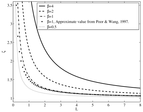
Figure 1: $\zeta$ vs. $\bar{L}$ for $\eta=\infty$ and a range of $\beta$, from (84).

VI-C Capacity Relationship

Consider the difference in capacity per data stream of the MMSE and the ALS receivers, defined as $\vartriangle\mathcal{C}_{\text{ALS}}^{k}=\log(1+\text{SINR}^{\text{MMSE}}_{k})-\log(1+\text{SINR}^{\text{ALS}}_{k})$. We have from (82) and (83)

$$\vartriangle\mathcal{C}_{\text{ALS}}^{k} =\ln\left(1+\left(1-\frac{1}{\zeta}\right)\text{SINR}^{\text{MMSE}}_{k}\right)$$ (91)

with semi-blind training, and

$$\vartriangle\mathcal{C}_{\text{ALS}}^{k} =\ln\left(1+\left(\frac{1-\frac{1}{\zeta}}{\frac{\text{SINR}^{\text{MMSE}}_{k}-1}{\zeta}+1}\right)\text{SINR}^{\text{MMSE}}_{k}\right)$$ (92)

with training sequences.

As $\zeta\to 1$, the capacity difference approaches zero, whereas as $\zeta\to\infty$, the difference approaches $\ln\left(1+\text{SINR}^{\text{MMSE}}_{k}\right)$. Recall that $\zeta$ only depends on $\eta$ (the ratio of training symbols to transmit dimensions), $\beta$ (the ratio of receive to transmit dimensions), and the window shape, and does not depend on the SNR, the (normalized) number of data streams $\alpha$, or the channel distribution. Nor does this value depend on whether ${\mathbf{S}}$ is i.i.d. or isometric. Fig. 1 shows the steady-state value of $\zeta$ vs. $\bar{L}$ with exponential windowing and a range of $\beta$ values.

VII Numerical Studies

We now present various applications of the results presented in previous sections. We shall focus on three example systems:

• The first is the standard model of a MIMO channel with rich scattering, for which we set ${\mathbf{H}}={\mathbf{I}}_{N}$ and ${\mathbf{S}}$ i.i.d., so that $K$ and $N$ represent the number of transmit and receive antennas, respectively.

• The second example system is CDMA in frequency-selective Rayleigh fading, for which ${\mathbf{S}}$ contains either i.i.d. or isometric signatures, and ${\mathbf{H}}$ is a square $N\times N$ matrix (hence $\beta=1$), for which the a.e.d. of the channel correlation matrix ${\mathbf{H}}^{\ddagger}$ is exponential with mean one (i.e., $f_{H}(h)=\exp(-h)$ for $h>0$ is the density used to compute the $\hat{\mathcal{H}}_{m,n}$ values).

• The third example system is a SISO FIR channel with a cyclic prefix, as described after Proposition 1 in Section II-E, where ${\mathbf{h}}=\left[0.227,\>0.46,\>0.688,\>0.46,\>0.227\right]^{\dagger}$ (i.e., where the ALS and MMSE receiver is used to equalize the so-called Proakis Channel-C [26, pp. 616]). That is, the empirical results will be obtained using ${\mathbf{H}}$ given by the circulant matrix obtained from ${\mathbf{h}}$, and ${\mathbf{S}}={\mathbf{A}}={\mathbf{I}}_{N}$. As described in Proposition 1, the analytic results are obtained from the isometric ${\mathbf{S}}$ equations with $\alpha=1$, and $H$ distributed according to the spectra of ${\mathbf{h}}$, i.e., $F_{H}(h)=\frac{1}{N}\sum_{n=1}^{N}u(h-\mathcal{Q}(n))$, where $u(t)$ is the step function, and $\mathcal{Q}(n)=\left|{\operatorname{DFT}_{N}^{n}({\mathbf{h}})}\right|^{2}$, where $\operatorname{DFT}_{N}^{n}({\mathbf{h}})$ denotes the $n^{\text{th}}$ element of the $N$-point discrete Fourier transform of ${\mathbf{h}}$.

Unless otherwise stated, we shall assume equal transmit power per data stream (i.e., ${\mathbf{A}}={\mathbf{I}}_{K}$), and SNR$=10$ dB, where SNR is defined as the energy transmitted per data stream in each symbol interval, divided by $\sigma^{2}$.

In the following plots we determine empirical values from averages of a size $N=32$ system with QPSK modulation for comparison with the large system results. The asymptotic values for the MMSE curves have been determined from Theorem 1, and the asymptotic values for the ALS curves have been determined from Theorem 2, Theorem 3, and Lemma 1. The steady-state values of the ALS receiver have been determined from Corollary 1. Where possible, the ALS SINR has been determined from the MMSE SINR using Theorem 4 (i.e., any situation with i.i.d. training sequences and no diagonal loading).

VII-A Transient ALS SINR response and comparison with empirical values

VII-A1 MIMO example

Firstly, we demonstrate the relevance of the large-system limit to practical finite systems. Fig. 2 shows both asymptotic and empirical values of MMSE and ALS SINR vs. training length for the example MIMO system with rich scattering. For the ALS receiver, the diagonal loading value is $\mu=0.1$, and rectangular windowing is used. Clearly, the empirical (finite) values match the analytic (asymptotic) values very closely.

Note that the orthogonal training sequences clearly outperform the i.i.d. training sequences, particularly for ‘small’ $\eta$. This gap also widens as the number of receive dimensions decreases. Also, the performance of the semi-blind ALS receiver is comparable to the performance of the ALS receiver with training for the 2 to 1 transmit to receive antennas ratio case, but is significantly worse in the 1 to 2 transmit to receive antennas ratio case.

 

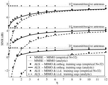
(a) ALS with training

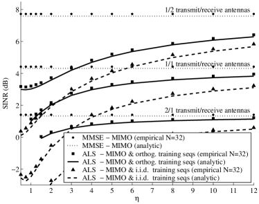
(b) semi-blind ALS

Figure 2: SINR vs. training length: (Rich MIMO) equal transmit power per antenna, SNR$=10$dB, $\mu=0.1$, rectangular windowing. Comparison with empirical values $N=32$, QPSK modulation.

VII-A2 CDMA in frequency-selective fading

Fig. 3 shows empirical and asymptotic values of MMSE and ALS SINR vs. $\eta$ for the example CDMA system in frequency-selective Rayleigh fading with $\alpha=0.50$. The ALS receiver uses rectangular windowing and a diagonal loading constant $\mu=0.1$. Curves are shown for both i.i.d. and isometric signatures, and i.i.d. and orthogonal training sequences. Again, the empirical (finite) values match the analytic (asymptotic) values.

Figure 3(b) shows the intuitively pleasing result that for a small number of training symbols (i.e., small $\eta$), orthogonal training sequences improve the performance of the ALS receiver more than isometric signatures, and as $\eta$ increases, this situation is quickly reversed. This is due to the fact that the $K$ i.i.d. training sequences of length $i$ become ‘more orthogonal’ as $i$ increases, and also since isometric signatures consistently outperform i.i.d. signatures.

In subsequent plots, we shall omit the empirical values, and concentrate on applications of the analytical results.

 

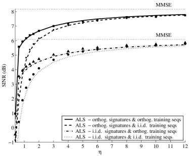
(a) ALS with training

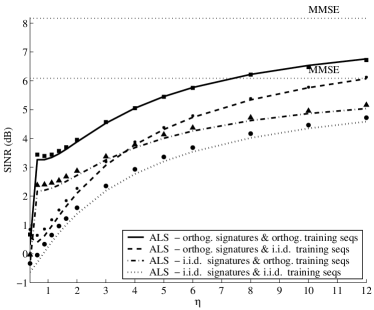
(b) semi-blind ALS

Figure 3: SINR vs. training length: CDMA in frequency-selective fading, SNR=10dB, $\alpha=0.50$, $\mu=0.1$, rectangular windowing, equal power per signature, exponential distribution for a.e.d. of ${\mathbf{H}}^{\ddagger}$. Comparison with empirical values $N=32$, QPSK modulation.

VII-A3 Equalization

Fig. 4 shows empirical and asymptotic values of MMSE and ALS SINR vs. $\eta$ for the example SISO FIR system at 20dB SNR. The ALS receiver uses exponential windowing and a diagonal loading constant $\mu=0.1$. Curves are shown for both i.i.d. and orthogonal training sequences. Note that Proposition 1 requires that ${\mathbf{b}}_{m}$ is unitarily invariant, whereas the empirical values in the figure are based on standard QPSK modulation (i.e., ${\mathbf{b}}_{m}$ is not unitarily invariant). Clearly, at least in this case, the asymptotic results are a very good approximation for non-unitarily invariant data vectors.

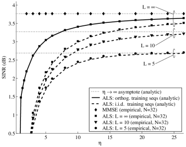
Figure 4: SINR vs. training length: Equalization of Proakis C-channel (i.e., ${\mathbf{H}}$ circulant matrix constructed from impulse response, and ${\mathbf{S}}={\mathbf{A}}={\mathbf{I}}_{N}$) at SNR=20dB. The ALS receiver uses $\mu=0.1$, exponential windowing, with training using i.i.d. and orthogonal training sequences. Comparison with empirical values $N=32$, QPSK modulation. Analytic values are obtained using isometric ${\mathbf{S}}$ equations with $\alpha=\beta=1$, as specified by Proposition 1.

VII-B Capacity with exponential windowing

Now we examine the performance of the ALS receiver with both rectangular and exponential windowing, relative to the MMSE receiver. Fig. 5 shows the capacity difference per-signature as a function of the window size $\bar{L}$ (determined from (91) and (92)) for the example CDMA system in frequency-selective Rayleigh fading with i.i.d. signatures, i.i.d. training, and a system load of $\alpha=0.75$. Curves for the ALS receiver are shown with both rectangular and exponential windowing, and diagonal loading constant $\mu=0$. Also, $f_{P}(p)=\frac{3}{4}\delta(p-1)+\frac{1}{4}\delta(p-\frac{1}{2})$, that is, one quarter of the signatures are transmitted at half the power of the remaining signatures.

In this figure, we do not take into account the loss in rate due to the training. This is considered in the following subsection. Rather, for a single channel use at a certain SNR, we wish to see the relative capacity difference between the MMSE receiver (using full CSI), and that obtained by the ALS receiver as a function of the number of training symbols used to generate the filter. Also, for the ALS receiver, we wish to compare exponential windowing with rectangular windowing at a given value of $\eta$ as a function of the exponential windowing window size, $\bar{L}$.

Firstly, we see that for either type of windowing, increasing the number of training symbols is an exercise in diminishing returns. Also, we see that as the window size increases, exponential windowing asymptotes to rectangular windowing, as would be expected for the time-invariant system model (1). Of course, exponential windowing is included to allow for time-varying channels. As such, the curves for exponential windowing are a valid approximation for a time-varying system in which the coherence time of the system is at least as large as the effective window size created by the exponential windowing. As such, the values of capacity or SINR obtained represent best possible values, which are only attained if the system remains static for the duration of the ALS training period. Extending these results to time-varying systems is an open problem, and is likely to be difficult.

 

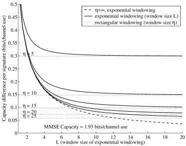
(a) ALS with training

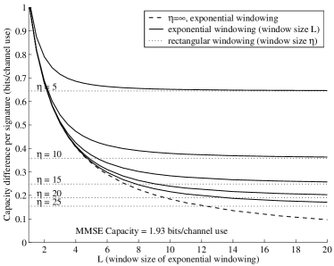
(b) semi-blind ALS

Figure 5: Capacity difference between ALS and MMSE receivers vs. window size of exponential window: CDMA in frequency-selective fading, i.i.d. signatures, i.i.d. training, SNR=10dB, $\alpha=0.75$, $\mu=0$, rectangular and exponential windowing. Note the window size for rectangular windowing is $\eta$. Also, $f_{P}(p)=\frac{3}{4}\delta(p-1)+\frac{1}{4}\delta(p-\frac{1}{2})$. Curves shown correspond to the first $3/4$ of the signatures. Note that the scale of the vertical axis of Fig. 5(b) is twice that of Fig. 5(a).

VII-C Application: Throughput Optimization

We now demonstrate how the results can be used to optimize the throughput with packet transmissions. More training symbols gives a higher ALS SINR, but leaves less room for data-carrying symbols in the packet. Clearly, there is an optimal ratio of training symbols to data-carrying symbols. Such an optimization has been considered for MIMO block fading channels and SISO FIR channels in [27, 28] with an optimal (maximum-likelihood) receiver. In that work, the training symbols are used to estimate the channel directly. A lower bound on the capacity is derived, and is used to optimize the training length. Related work in [29] applies the large-system transient analysis in [16] for the MIMO i.i.d. channel to optimize the training length with an ALS receiver (without exponential windowing or diagonal loading). It is shown there that for large packet lengths ($\ell$) the training length that maximizes capacity grows as $\operatorname{O}(\sqrt{\ell})$. Optimization of power levels between the training and data symbols is also investigated.

Suppose we consider a packet containing $T>i$ symbols, of which the first $i$ are training symbols, and the remainder consists of data-carrying symbols. There are $K$ equal power data streams, which are coded independently with capacity-achieving codes with rate $R_{c}=\log_{2}(1+\text{SINR}^{\text{ALS}})$. We focus on the ALS receiver with known training symbols. The number of information bits per block is therefore $KR_{c}(T-i)$, while the number of transmit dimensions per block is $NT$. Therefore, the number of information bits per transmit dimension (hereafter referred to as ‘normalized capacity’) is $C=\alpha R_{\text{eff}}$, where $R_{\text{eff}}=R_{c}(1-\eta/\ell)$ and $\ell=T/N$. We shall consider the additional limit $T\to\infty$ with $T/N\to\ell>0$ in order to optimize $C$ with respect to the normalized training length $\eta$. We shall keep $E_{b}/\sigma^{2}=\textsf{SNR}/R_{\text{eff}}$ constant, and unless otherwise stated, in the numerical examples $E_{b}/\sigma^{2}$ = 10 dB.

Fig. 6(a) shows the normalized capacity of the example CDMA system in frequency-selective fading as a function of $\eta$ and $\alpha$ for a normalized block length of $\ell=T/N=15$. The ALS receiver uses rectangular windowing and no diagonal loading. Fig. 6(b) shows the additional normalized capacity obtained, relative to the results for i.i.d. training in Fig. 6(a), if orthogonal training sequences are used. Although not shown, plots analogous to Fig. 6 may also be obtained for isometric ${\mathbf{S}}$.

Fig. 6(a) shows that there is an optimum value of $\eta/\ell$, i.e., the ratio of training length to block length, for each value of system load, $\alpha$. Fig. 7(a) shows the value of normalized capacity at the optimum value of $\eta$, again for $\ell=15$, as a function of the system load $\alpha$. Fig. 7(b) shows the corresponding value of $\eta$ (expressed as a percentage of $\ell$) which maximizes the normalized capacity. Also shown in Fig. 7(a) is the normalized capacity of the MMSE receiver at the same value of $E_{b}/\sigma^{2}$, for both types of signatures. Of course, the MMSE receiver assumes perfect CSI.

 

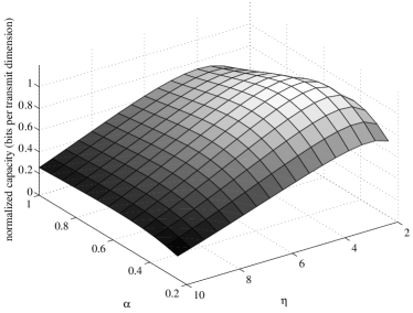
(a) i.i.d. training signatures

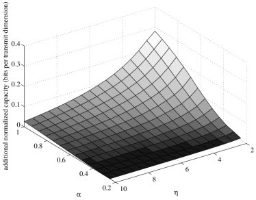
(b) Additional normalized capacity obtained using orthogonal training signatures

Figure 6: Throughput optimization: CDMA in frequency-selective fading, i.i.d. ${\mathbf{S}}$, normalized block length $T/N=15$, rectangular windowing, no diagonal loading, $\frac{E_{b}}{\sigma^{2}}$=10 dB. Fig. 6(b) shows the additional normalized capacity (with respect to Fig. 6(a)) obtained if orthogonal training sequences are used.

 

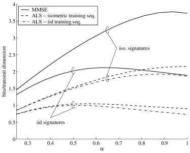
(a) Optimal Throughput

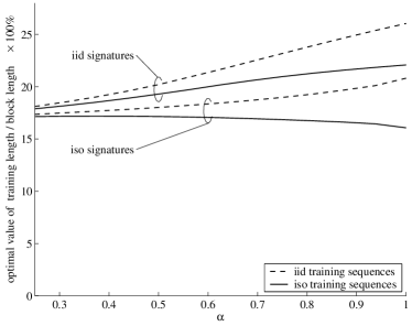
(b) Optimal Training Length

Figure 7: Throughput optimization: CDMA in frequency-selective fading, normalized block length $T/N=15$, rectangular windowing, no diagonal loading, $\frac{E_{b}}{\sigma^{2}}$=10 dB, equal power per signature, exponential distribution for a.e.d. of ${\mathbf{H}}^{\ddagger}$.

We now consider throughput optimization for the example MIMO system, and consider the growth in normalized capacity with respect to the normalized block length, $\ell$. In this example, since $K$ represents the number of transmit dimensions, the number of transmit dimensions per block is $KT$, and hence the number of information bits per transmit dimension is $C=R_{\text{eff}}$. Figure 8(a) shows the growth in normalized capacity, optimized with respect to $\eta/\ell$. These results show that the gain in using orthogonal training sequences appears to be more pronounced in situations where there is a high ratio of transmit antennas to receive antennas (i.e., $\alpha>1$). Figure 8(b) shows the associated optimal training length $\eta$, expressed as a percentage of the block length $\ell$, for i.i.d. training sequences.

Figure 9 shows the optimal value of $\eta$ for orthogonal training sequences corresponding to the curves in Figure 8(a).

It is interesting to note the case $\alpha=4$, where we see that $\eta$ is never chosen less than $4$. Recall that for $\alpha>\eta$, we have orthogonal rows of ${\mathbf{B}}$ and for $\alpha<\eta$, we have orthogonal columns of ${\mathbf{B}}$. Clearly, orthogonal columns are preferable. If the axis were extended, we would see the same behavior in the other curves.

 

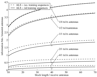
(a) Throughput

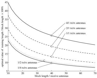
(b) Optimal percentage of training in a block (i.i.d. training)

Figure 8: Throughput optimization: MIMO channel, rectangular windowing, no diagonal loading, $\frac{E_{b}}{\sigma^{2}}$=10 dB, equal transmit power per antenna.

Figure 9: Optimal value of normalized training length $\eta$ for orthogonal training sequences corresponding to Figure 8(a).

VIII Conclusions

Determining the transient behavior of ALS algorithms with random inputs is a classical problem, which is relevant to many communications applications, such as equalization and interference suppression. The large system results presented here are the first set of exact results, which characterize the transient performance of ALS algorithms for a wide variety of channel models of interest. Namely, our results apply to any linear input-output model (see Proposition 1), where the input is unitarily invariant, and the channel matrix has a well-defined a.e.d. with finite moments. As such, these results can be used to evaluate adaptive equalizer performance in the context of space-time channels. This represents a significant generalization of the previous large system results in [16], which apply only to an i.i.d. channel matrix. Furthermore, the analytical approach relies only on elementary matrix manipulations, and is general enough to allow for orthonormal spreading and/or training sequences, in addition to i.i.d. sequences. Numerical results were presented, which show that orthogonal training sequences can perform significantly better than i.i.d. training sequences.

For the general ALS algorithm and model considered, the output SINR can be expressed as the solution to a set of nonlinear equations. These equations are complicated by the fact that they depend on a number of auxiliary variables, each of which is a particular large matrix moment involving the sample covariance matrix. Still, it is relatively straightforward to solve these equations numerically. Illustrative examples were presented showing the effect of training length on the capacity of a block fading channel.

In the case of i.i.d. sequences without diagonal loading, the set of equations for output SINR yields a simple relationship between the SINRs for ALS and MMSE receivers, which accounts for an arbitrary data shaping window. This relation shows that ALS performance depends on the channel matrix only through the MMSE. In other words, ALS performance is independent of the channel shape given a target output MMSE. Whether or not an analogous relation holds with diagonal loading, orthogonal training and/or spreading sequences remains an open problem. Application of the analysis presented here to more general channel models (e.g., multi-user/multi-antenna) is also a topic for further study.

Appendix A Precursor to Asymptotic Analysis

Definition 1

Let $\{a_{N}\}_{N=1,\ldots}$ and $\{b_{N}\}_{N=1,\ldots}$ denote a pair of infinite sequences of complex-valued random variables indexed by $N$. These sequences are defined to be asymptotically equivalent, denoted $a_{N}\asymp b_{N}$, iff $\left|{a_{N}-b_{N}}\right|\stackrel{{\scriptstyle a.s.}}{{\longrightarrow}}0$ as $N\to\infty$, where $\stackrel{{\scriptstyle a.s.}}{{\longrightarrow}}$ denotes almost-sure convergence in the limit considered. $\Box$

Clearly $\asymp$ is an equivalence relation, transitivity being obtained through the triangle inequality. We shall additionally define asymptotic equivalence for sequences of $N\times 1$ vectors and $N\times N$ matrices in an identical manner as above, where the absolute value is replaced by the Euclidean vector norm and the associated induced spectral norm, respectively.

Lemma 2

If $a_{N}\asymp b_{N}$ and $x_{N}\asymp y_{N}$, and if $\left|{a_{N}}\right|$, $\left|{y_{N}}\right|$ and/or $\left|{b_{N}}\right|$, $\left|{x_{N}}\right|$ are almost surely uniformly bounded above over $N$, then $a_{N}x_{N}\asymp b_{N}y_{N}$. Similarly, $a_{N}/x_{N}\asymp b_{N}/y_{N}$ if $\left|{a_{N}}\right|$ or $\left|{b_{N}}\right|$ is uniformly bounded above over $N$, and at least one of $\inf_{N}\left|{x_{N}}\right|$ and $\inf_{N}\left|{y_{N}}\right|$ is positive almost surely.

Proof:

The fact that $a_{N}x_{N}\asymp b_{N}y_{N}$ can be seen after writing $a_{N}x_{N}-b_{N}y_{N}=a_{N}x_{N}-b_{N}y_{N}+a_{N}y_{N}-a_{N}y_{N}$ and hence $\left|{a_{N}x_{N}-b_{N}y_{N}}\right|\leq\left|{a_{N}}\right|\left|{x_{N}-y_{N}}\right|+\left|{y_{N}}\right|\left|{a_{N}-b_{N}}\right|$. Alternatively, we may add and subtract $b_{N}x_{N}$ from $a_{N}x_{N}-b_{N}y_{N}$ to obtain $\left|{a_{N}x_{N}-b_{N}y_{N}}\right|\leq\left|{x_{N}}\right|\left|{a_{N}-b_{N}}\right|+\left|{b_{N}}\right|\left|{x_{N}-y_{N}}\right|$. The division property, $a_{N}/x_{N}\asymp b_{N}/y_{N}$, can be shown in the same way

$$\left|{\frac{a_{N}}{x_{N}}-\frac{b_{N}}{y_{N}}}\right| \leq\begin{cases}\frac{\left|{a_{N}}\right|\left|{x_{N}-y_{N}}\right|}{\left|{x_{N}}\right|\left|{y_{N}}\right|}+\frac{\left|{a_{N}-b_{N}}\right|}{\left|{y_{N}}\right|}\\ \frac{\left|{b_{N}}\right|\left|{x_{N}-y_{N}}\right|}{\left|{x_{N}}\right|\left|{y_{N}}\right|}+\frac{\left|{a_{N}-b_{N}}\right|}{\left|{x_{N}}\right|}\end{cases}$$ (93)

Suppose $\delta=\inf_{N}\left|{y_{N}}\right|$. Given a realization for which $\left|{x_{N}-y_{N}}\right|\to 0$ and $\delta>0$, we may take $N$ sufficiently large such that $\left|{x_{N}-y_{N}}\right|\leq\delta/2$ and hence $\left|{x_{N}}\right|\geq\delta/2$. Alternatively, for a realization for which $\left|{x_{N}-y_{N}}\right|\to 0$ and $\delta^{\prime}=\inf_{N}\left|{x_{N}}\right|>0$, for $N$ sufficiently large we may show $\left|{y_{N}}\right|\geq\delta^{\prime}/2$. Using these facts, and the uniform upper bounds for $\left|{a_{N}}\right|$ or $\left|{b_{N}}\right|$ we obtain the result.         

Note that the multiplicative part of Lemma 2 holds for any mixture of matrices, vectors or scalars for which the dimensions of $a_{N}$ and $x_{N}$ are such that $a_{N}x_{N}$ makes sense, due to the submultiplicative property of the spectral norm. The following definition and related results, however, are concerned with scalar complex sequences.

Definition 2

Let $\{\{a_{N,n}\}_{n=1\ldots N}\}_{N=1,\ldots}$ and $\{\{b_{N,n}\}_{n=1\ldots N}\}_{N=1,\ldots}$ denote a pair of infinite sequences, indexed by $N$. The $N^{\text{th}}$ element is a complex-valued sequences of length $N$, indexed by $n$. These sequences are defined to be uniformly asymptotically equivalent, denoted $a_{N,n}\stackrel{{\scriptstyle n}}{{\asymp}}b_{N,n}$, iff $\max_{n\leq N}\left|{a_{N,n}-b_{N,n}}\right|\stackrel{{\scriptstyle a.s.}}{{\longrightarrow}}0$ as $N\to\infty$. $\Box$

Also we define $a_{N}$ and $b_{N,n}$ (as defined in Definitions 1 and 2 above) as being uniformly asymptotically equivalent (denoted $a_{N}\stackrel{{\scriptstyle n}}{{\asymp}}b_{N,n}$), if $a_{N,n}\stackrel{{\scriptstyle n}}{{\asymp}}b_{N,n}$ where $a_{N,n}=a_{N}$ for all $n=1,\ldots,N$.

Also, analogous to Lemma 2, we have

Lemma 3

If $a_{N,n}\stackrel{{\scriptstyle n}}{{\asymp}}b_{N,n}$ and $x_{N,n}\stackrel{{\scriptstyle n}}{{\asymp}}y_{N,n}$, and if $\left|{a_{N,n}}\right|$, $\left|{y_{N,n}}\right|$ and/or $\left|{b_{N,n}}\right|$, $\left|{x_{N,n}}\right|$ are almost surely uniformly bounded above over $N$ and $n$, then $a_{N,n}x_{N,n}\stackrel{{\scriptstyle n}}{{\asymp}}b_{N,n}y_{N,n}$. Similarly, $a_{N,n}/x_{N,n}\stackrel{{\scriptstyle n}}{{\asymp}}b_{N,n}/y_{N,n}$ if $\left|{a_{N,n}}\right|$ or $\left|{b_{N,n}}\right|$ is almost surely uniformly bounded above over $N$ and $n$, and at least one of $\inf_{N,n}\left|{x_{N,n}}\right|$ and $\inf_{N,n}\left|{y_{N,n}}\right|$ is positive almost surely.

Lemma 4

If $a_{N,n}\stackrel{{\scriptstyle n}}{{\asymp}}b_{N,n}$, then $\frac{1}{N}\sum_{n=1}^{N}a_{N,n}\asymp\frac{1}{N}\sum_{n=1}^{N}b_{N,n}$.

Proof:

This follows immediately from

$$\left|{\frac{1}{N}\sum_{n=1}^{N}(a_{N,n}-b_{N,n})}\right| \leq\max_{n\leq N}\left|{a_{N,n}-b_{N,n}}\right|$$ (94)

        

Lemma 5

For $N=1,\ldots$, let ${\mathbf{X}}_{N}={\mathbf{M}}_{N}-z{\mathbf{I}}_{N}$, where ${\mathbf{M}}_{N}$ is an $N\times N$ Hermitian matrix and $z\in{\Bbb{C}}^{+}$, and suppose ${\mathbf{u}}_{N}\in{\Bbb{C}}^{N}$. Denote $u_{N}={\mathbf{u}}_{N}^{\dagger}{\mathbf{X}}_{N}^{-1}{\mathbf{u}}_{N}$. If

$$b=\inf_{N} \left|{{\mathbf{u}}_{N}}\right|>0\quad\text{, a.s.}$$ (95)

$$B=\sup_{N} \|{{\mathbf{X}}_{N}}\|<\infty\quad\text{, a.s.}$$ (96)

Then

$$\operatorname{Im}(u_{N})\geq\operatorname{Im}(z)\frac{b^{2}}{B^{2}}\quad\text{, a.s.}$$ (97)

and hence $u_{N}\in{\Bbb{C}}^{+}$, almost surely.

Proof:

First, we note the inequality (from the proof of [30, Lemma 16.5])

$$\frac{{\mathbf{x}}^{\dagger}{\mathbf{x}}}{{\mathbf{x}}^{\dagger}{\mathbf{Y}}^{-1}{\mathbf{x}}} \leq\frac{{\mathbf{x}}^{\dagger}{\mathbf{Y}}{\mathbf{x}}}{{\mathbf{x}}^{\dagger}{\mathbf{x}}}$$ (98)

for any ${\mathbf{x}}\in{\Bbb{C}}^{N}$, ${\mathbf{x}}\neq\mathbf{0}$, and Hermitian positive definite $N\times N$ complex-valued matrix ${\mathbf{Y}}$.

Now,

$$\operatorname{Im}(u_{N}) =\frac{1}{2\mathbf{j}}{\mathbf{u}}_{N}^{\dagger}({\mathbf{X}}^{-1}-{\mathbf{X}}^{-{\dagger}}){\mathbf{u}}_{N}\>=\>\operatorname{Im}(z){\mathbf{u}}_{N}^{\dagger}({\mathbf{X}}^{\dagger}{\mathbf{X}})^{-1}{\mathbf{u}}_{N}$$ (99)

and hence using (98) and a realization for which (95) and (96) holds we obtain

$$\frac{1}{\operatorname{Im}(u_{N})} =\frac{1}{\operatorname{Im}(z){\mathbf{u}}_{N}^{\dagger}({\mathbf{X}}^{\dagger}{\mathbf{X}})^{-1}{\mathbf{u}}_{N}}\;\leq\;\frac{{\mathbf{u}}_{N}^{\dagger}{\mathbf{X}}^{\dagger}{\mathbf{X}}{\mathbf{u}}_{N}}{\operatorname{Im}(z)({\mathbf{u}}_{N}^{\dagger}{\mathbf{u}}_{N})^{2}}\;\leq\;\frac{\|{{\mathbf{X}}}\|^{2}}{\operatorname{Im}(z)\left|{{\mathbf{u}}_{N}}\right|^{2}}$$ (100)

which, with (95), (96), and $z\in{\Bbb{C}}^{+}$ gives the result.         

The following lemma is an asymptotic extension of the matrix inversion lemma, and is used extensively in the subsequent appendices to remove matrix dimensions as described in Section III. It is based on an approach in [16].

Lemma 6

Let ${\mathbf{Y}}_{N}={\mathbf{X}}_{N}+{\mathbf{v}}_{N}{\mathbf{u}}_{N}^{\dagger}+{\mathbf{u}}_{N}{\mathbf{v}}_{N}^{\dagger}+c_{N}{\mathbf{u}}_{N}{\mathbf{u}}_{N}^{\dagger}$, where ${\mathbf{v}}_{N},{\mathbf{u}}_{N}\in{\Bbb{C}}^{N}$, $c_{N}\in{\Bbb{R}}^{*}$, and ${\mathbf{X}}_{N}={\mathbf{M}}_{N}-z{\mathbf{I}}_{N}$, where ${\mathbf{M}}_{N}$ is an $N\times N$ Hermitian matrix and $z\in{\Bbb{C}}^{+}$. Denote

$$\epsilon_{N} ={\mathbf{u}}_{N}^{\dagger}{\mathbf{X}}_{N}^{-1}{\mathbf{v}}_{N}$$ (101)

$$u_{N} ={\mathbf{u}}_{N}^{\dagger}{\mathbf{X}}_{N}^{-1}{\mathbf{u}}_{N}$$ (102)

$$v_{N} ={\mathbf{v}}_{N}^{\dagger}{\mathbf{X}}_{N}^{-1}{\mathbf{v}}_{N}$$ (103)

Assume that as $N\to\infty$,

$$|\epsilon_{N}| \stackrel{{\scriptstyle a.s.}}{{\longrightarrow}}0$$ (104)

and

$$b\>=\>\inf_{N} \left|{{\mathbf{u}}_{N}}\right|>0\quad\text{, a.s.,}$$ (105)

$$B\>=\>\sup_{N} \max\left\{\|{{\mathbf{X}}_{N}}\|,\>\left|{{\mathbf{v}}_{N}}\right|,\>\left|{{\mathbf{u}}_{N}}\right|,\>\left|{c_{N}}\right|\right\}<\infty\quad\text{, a.s.}$$ (106)

Then,

$$\left|{{\mathbf{Y}}_{N}^{-1}{\mathbf{u}}_{N}-\frac{{\mathbf{X}}_{N}^{-1}({\mathbf{u}}_{N}-u_{N}{\mathbf{v}}_{N})}{1-u_{N}(v_{N}-c_{N})}}\right|\stackrel{{\scriptstyle a.s.}}{{\longrightarrow}}0$$ (107)

$$\left|{{\mathbf{Y}}_{N}^{-1}{\mathbf{v}}_{N}-\frac{{\mathbf{X}}_{N}^{-1}(-v_{N}{\mathbf{u}}_{N}+(1+c_{N}u_{N}){\mathbf{v}}_{N})}{1-u_{N}(v_{N}-c_{N})}}\right|\stackrel{{\scriptstyle a.s.}}{{\longrightarrow}}0$$ (108)

as $N\to\infty$, and

$$\delta =\inf_{N}\min\left\{\left|{1-u_{N}v_{N}}\right|,\;\left|{1-u_{N}(v_{N}-c_{N})}\right|\right\}\;>\;0$$ (109)

almost surely, where $\delta$ depends only on $B$, $b$, and $\operatorname{Im}(z)$.

Proof:

First note that from Lemma 5, (105), and (106), that $u_{N}\in{\Bbb{C}}^{+}$ almost surely. We therefore consider a realization for which $u_{N}\in{\Bbb{C}}^{+}$ and (104)–(106) holds, and take $N$ sufficiently large such that $\left|{\epsilon_{N}}\right|\leq 1/2$ and hence

$$\left|{1+\epsilon_{N}}\right|\geq 1/2.$$ (110)

Due to the definition of ${\mathbf{X}}$,

$$\|{{\mathbf{X}}^{-1}}\|\leq\operatorname{Im}(z)^{-1}.$$ (111)

Now note that $\sup_{N}\left|{u_{N}}\right|=B^{2}\operatorname{Im}(z)^{-1}<\infty$ due to (106) and (111). Also, $\operatorname{Im}(-u_{N}^{-1})=\operatorname{Im}(u_{N})/\left|{u_{N}}\right|^{2}$ and $\sup_{N}\left|{u_{N}^{-1}}\right|=\operatorname{Im}(u_{N})^{-1}$. Additionally, note that $\operatorname{Im}(v_{N})\geq 0$, using an identical argument to (99). Using these facts we obtain

$$\left|{\frac{1}{1-u_{N}v_{N}}}\right| =\frac{\left|{-u_{N}^{-1}}\right|}{\left|{-u_{N}^{-1}+v_{N}}\right|}\leq\frac{\left|{u_{N}^{-1}}\right|}{\operatorname{Im}(-u_{N}^{-1}+v_{N})}\leq\frac{\left|{u_{N}^{-1}}\right|}{\operatorname{Im}(-u_{N}^{-1})}\>\leq\>\frac{\left|{u_{N}}\right|^{2}}{\operatorname{Im}(u_{N})^{2}}\leq\left(\frac{B^{2}}{\operatorname{Im}(z)b}\right)^{4}$$ (112)

In the same way, also using $c_{N}\in{\Bbb{R}}^{*}$, we obtain an identical uniform upper bound on $\left|{1-u_{N}(v_{N}-c_{N})}\right|^{-1}$, and hence obtain (109).

In what follows, we will drop the dependence on $N$ from $u_{N}$, $v_{N}$, $c_{N}$, ${\mathbf{u}}_{N}$, ${\mathbf{v}}_{N}$, ${\mathbf{X}}_{N}$, and ${\mathbf{Y}}_{N}$ to clarify the derivations. Define ${\mathbf{X}}_{1}$ and ${\mathbf{X}}_{2}$ according to the following equations

$${\mathbf{Y}} ={\mathbf{X}}_{2}+c{\mathbf{u}}{\mathbf{u}}^{\dagger}$$ (113)

$${\mathbf{X}}_{2} ={\mathbf{X}}_{1}+{\mathbf{u}}{\mathbf{v}}^{\dagger}$$ (114)

$${\mathbf{X}}_{1} ={\mathbf{X}}+{\mathbf{v}}{\mathbf{u}}^{\dagger}.$$ (115)

The matrix inversion lemma gives

$${\mathbf{Y}}^{-1} ={\mathbf{X}}_{2}^{-1}-\frac{c{\mathbf{X}}_{2}^{-1}{\mathbf{u}}{\mathbf{u}}^{\dagger}{\mathbf{X}}_{2}^{-1}}{1+c{\mathbf{u}}^{\dagger}{\mathbf{X}}_{2}^{-1}{\mathbf{u}}}$$ (116)

$${\mathbf{X}}_{2}^{-1} ={\mathbf{X}}_{1}^{-1}-\frac{{\mathbf{X}}_{1}^{-1}{\mathbf{u}}{\mathbf{v}}^{\dagger}{\mathbf{X}}_{1}^{-1}}{1+{\mathbf{v}}^{\dagger}{\mathbf{X}}_{1}^{-1}{\mathbf{u}}}$$ (117)

$${\mathbf{X}}_{1}^{-1} ={\mathbf{X}}^{-1}-\frac{{\mathbf{X}}^{-1}{\mathbf{v}}{\mathbf{u}}^{\dagger}{\mathbf{X}}^{-1}}{1+{\mathbf{u}}^{\dagger}{\mathbf{X}}^{-1}{\mathbf{v}}}.$$ (118)

First consider ${\mathbf{X}}_{1}^{-1}$, and note from (118), (104), Lemma 2, (106), (110), and (111) that

$${\mathbf{X}}_{1}^{-1} \asymp{\mathbf{X}}^{-1}-{\mathbf{X}}^{-1}{\mathbf{v}}{\mathbf{u}}^{\dagger}{\mathbf{X}}^{-1}$$ (119)

In fact, in the remainder of the proof, we shall repeatedly use (104), (106), (109), (110), and (111) in order to apply Lemma 2, without explicitly stating this, however, it should be clear from the context.

From (119) we obtain

$${\mathbf{X}}_{1}^{-1}{\mathbf{u}} \asymp{\mathbf{X}}^{-1}({\mathbf{u}}-u{\mathbf{v}})$$ (120)

$${\mathbf{X}}_{1}^{-1}{\mathbf{v}} \asymp{\mathbf{X}}^{-1}{\mathbf{v}}$$ (121)

$${\mathbf{v}}^{\dagger}{\mathbf{X}}_{1}^{-1} \asymp({\mathbf{v}}^{\dagger}-v{\mathbf{u}}^{\dagger}){\mathbf{X}}^{-1}$$ (122)

$${\mathbf{u}}^{\dagger}{\mathbf{X}}_{1}^{-1} \asymp{\mathbf{u}}^{\dagger}{\mathbf{X}}^{-1}$$ (123)

From this, we obtain

$${\mathbf{u}}^{\dagger}{\mathbf{X}}_{1}^{-1}{\mathbf{u}} \asymp u$$ (124)

$${\mathbf{v}}^{\dagger}{\mathbf{X}}_{1}^{-1}{\mathbf{v}} \asymp v$$ (125)

$${\mathbf{v}}^{\dagger}{\mathbf{X}}_{1}^{-1}{\mathbf{u}} \asymp-uv$$ (126)

$${\mathbf{u}}^{\dagger}{\mathbf{X}}_{1}^{-1}{\mathbf{v}} \asymp 0$$ (127)

Before we consider ${\mathbf{X}}_{2}^{-1}$, we first analyze the denominator of the second term in (117). Firstly, due to (126), we may take $N$ large enough such that $\left|{{\mathbf{v}}^{\dagger}{\mathbf{X}}_{1}^{-1}{\mathbf{u}}+uv}\right|<\delta/2$, and hence with (109) we obtain $\left|{1+{\mathbf{v}}^{\dagger}{\mathbf{X}}_{1}^{-1}{\mathbf{u}}}\right|\geq\delta/2$. With this fact, we obtain $(1+{\mathbf{v}}^{\dagger}{\mathbf{X}}_{1}^{-1}{\mathbf{u}})^{-1}\asymp(1-uv)^{-1}$, since

$$\left|{\frac{1}{1+{\mathbf{v}}^{\dagger}{\mathbf{X}}_{1}^{-1}{\mathbf{u}}}-\frac{1}{1-uv}}\right| =\frac{\left|{{\mathbf{v}}^{\dagger}{\mathbf{X}}_{1}^{-1}{\mathbf{u}}+uv}\right|}{\left|{1+{\mathbf{v}}^{\dagger}{\mathbf{X}}_{1}^{-1}{\mathbf{u}}}\right|\left|{1-uv}\right|}\>\leq\>\frac{2}{\delta^{2}}\left|{{\mathbf{v}}^{\dagger}{\mathbf{X}}_{1}^{-1}{\mathbf{u}}+uv}\right|$$ (128)

Now consider ${\mathbf{X}}_{2}^{-1}$, for which from (117) and the preceding discussion we obtain

$${\mathbf{X}}_{2}^{-1}{\mathbf{v}} ={\mathbf{X}}_{1}^{-1}{\mathbf{v}}-\frac{{\mathbf{X}}_{1}^{-1}{\mathbf{u}}{\mathbf{v}}^{\dagger}{\mathbf{X}}_{1}^{-1}{\mathbf{v}}}{1+{\mathbf{v}}^{\dagger}{\mathbf{X}}_{1}^{-1}{\mathbf{u}}}$$ (129)

$$\asymp{\mathbf{X}}_{1}^{-1}{\mathbf{v}}-\frac{v{\mathbf{X}}_{1}^{-1}{\mathbf{u}}}{1-uv}$$ (130)

$$\asymp\frac{1}{1-uv}{\mathbf{X}}^{-1}(-v{\mathbf{u}}+{\mathbf{v}})$$ (131)

Similarly,

$${\mathbf{X}}_{2}^{-1}{\mathbf{u}} \asymp\frac{1}{1-uv}{\mathbf{X}}^{-1}({\mathbf{u}}-u{\mathbf{v}})$$ (132)

$${\mathbf{v}}^{\dagger}{\mathbf{X}}_{2}^{-1} \asymp\frac{1}{1-uv}(-v{\mathbf{u}}^{\dagger}+{\mathbf{v}}^{\dagger}){\mathbf{X}}^{-1}$$ (133)

$${\mathbf{u}}^{\dagger}{\mathbf{X}}_{2}^{-1} \asymp\frac{1}{1-uv}({\mathbf{u}}^{\dagger}-u{\mathbf{v}}^{\dagger}){\mathbf{X}}^{-1}$$ (134)

and so,

$${\mathbf{u}}^{\dagger}{\mathbf{X}}_{2}^{-1}{\mathbf{v}} \asymp{\mathbf{v}}^{\dagger}{\mathbf{X}}_{2}^{-1}{\mathbf{u}}\>\asymp\>-\frac{vu}{1-uv}$$ (135)

$${\mathbf{u}}^{\dagger}{\mathbf{X}}_{2}^{-1}{\mathbf{u}} \asymp\frac{u}{1-uv}$$ (136)

$${\mathbf{v}}^{\dagger}{\mathbf{X}}_{2}^{-1}{\mathbf{v}} \asymp\frac{v}{1-uv}$$ (137)

$$1+c{\mathbf{u}}^{\dagger}{\mathbf{X}}_{2}^{-1}{\mathbf{u}} \asymp\frac{1-u(v-c)}{1-uv}$$ (138)

Before considering ${\mathbf{Y}}^{-1}$, we note that from (106), (109), (138), and similar arguments preceding (128) that $\left|{1+c{\mathbf{u}}^{\dagger}{\mathbf{X}}_{2}^{-1}{\mathbf{u}}}\right|$ has a positive uniform lower bound and $1/(1+c{\mathbf{u}}^{\dagger}{\mathbf{X}}_{2}^{-1}{\mathbf{u}})\asymp(1-uv)/(1-u(v-c))$.

Considering ${\mathbf{Y}}^{-1}$ using (116) and the preceding discussion, we obtain

$${\mathbf{Y}}^{-1}{\mathbf{u}} =\frac{{\mathbf{X}}_{2}^{-1}{\mathbf{u}}}{1+c{\mathbf{u}}^{\dagger}{\mathbf{X}}_{2}^{-1}{\mathbf{u}}}$$ (139)

$$\asymp\frac{1}{1-u(v-c)}{\mathbf{X}}^{-1}({\mathbf{u}}-u{\mathbf{v}}).$$ (140)

Similarly,

$${\mathbf{Y}}^{-1}{\mathbf{v}} ={\mathbf{X}}_{2}^{-1}{\mathbf{v}}-c\frac{{\mathbf{u}}^{\dagger}{\mathbf{X}}_{2}^{-1}{\mathbf{v}}}{1+c{\mathbf{u}}^{\dagger}{\mathbf{X}}_{2}^{-1}{\mathbf{u}}}{\mathbf{X}}_{2}^{-1}{\mathbf{u}}$$ (141)

$$\asymp{\mathbf{X}}_{2}^{-1}{\mathbf{v}}+c\frac{vu}{1-u(v-c)}{\mathbf{X}}_{2}^{-1}{\mathbf{u}}$$ (142)

$$\asymp\frac{1}{1-u(v-c)}{\mathbf{X}}^{-1}(-v{\mathbf{u}}+(1+uc){\mathbf{v}})$$ (143)

        

Lemma 7

Let ${\mathbf{A}}_{N}$ be an $N\times N$ Hermitian matrix, and suppose $A=\sup_{N}\|{{\mathbf{A}}_{N}}\|<\infty$. Using the definitions and assumptions of Lemma 6, additionally define

$$\varepsilon^{(1)}_{N} ={\mathbf{u}}_{N}^{\dagger}{\mathbf{X}}_{N}^{-1}{\mathbf{A}}_{N}{\mathbf{X}}_{N}^{-1}{\mathbf{v}}_{N}$$ (144)

$$\varepsilon^{(2)}_{N} ={\mathbf{v}}_{N}^{\dagger}{\mathbf{X}}_{N}^{-1}{\mathbf{A}}_{N}{\mathbf{X}}_{N}^{-1}{\mathbf{u}}_{N}$$ (145)

$$\acute{u}_{N} ={\mathbf{u}}_{N}^{\dagger}{\mathbf{X}}_{N}^{-1}{\mathbf{A}}_{N}{\mathbf{X}}_{N}^{-1}{\mathbf{u}}_{N}$$ (146)

$$\acute{v}_{N} ={\mathbf{v}}_{N}^{\dagger}{\mathbf{X}}_{N}^{-1}{\mathbf{A}}_{N}{\mathbf{X}}_{N}^{-1}{\mathbf{v}}_{N}$$ (147)

Then,

$$\left|{\mathrm{tr}[{\mathbf{A}}_{N}{\mathbf{Y}}_{N}^{-1}]-\left(\mathrm{tr}[{\mathbf{A}}_{N}{\mathbf{X}}_{N}^{-1}]+\frac{u_{N}\acute{v}_{N}+(v_{N}-c_{N})\acute{u}_{N}-\varepsilon^{(1)}_{N}-\varepsilon^{(2)}_{N}}{1-u_{N}(v_{N}-c_{N})}\right)}\right|\stackrel{{\scriptstyle a.s.}}{{\longrightarrow}}0$$ (148)

as $N\to\infty$.

Proof:

The proof continues from the proof of Lemma 6. Again, we drop the subscript $N$ for convenience. We see from (104), (118), (110) and (144) that

$$\mathrm{tr}[{\mathbf{A}}{\mathbf{X}}_{1}^{-1}] \asymp\mathrm{tr}[{\mathbf{A}}{\mathbf{X}}^{-1}]-\varepsilon^{(1)}$$ (149)

while (117), (120), (122), (126), and (144)–(147) give

$$\mathrm{tr}[{\mathbf{A}}{\mathbf{X}}_{2}^{-1}] \asymp\mathrm{tr}[{\mathbf{A}}{\mathbf{X}}_{1}^{-1}]-\frac{({\mathbf{v}}^{\dagger}-v{\mathbf{u}}^{\dagger}){\mathbf{X}}^{-1}{\mathbf{A}}{\mathbf{X}}^{-1}({\mathbf{u}}-u{\mathbf{v}})}{1-uv}$$ (150)

$$=\mathrm{tr}[{\mathbf{A}}{\mathbf{X}}_{1}^{-1}]+\frac{u\acute{v}+v\acute{u}-\varepsilon^{(2)}-uv\varepsilon^{(1)}}{1-uv}.$$ (151)

Similarly, (132), (134) and (144)–(147) give

$${\mathbf{u}}^{\dagger}{\mathbf{X}}_{2}^{-1}{\mathbf{A}}{\mathbf{X}}_{2}^{-1}{\mathbf{u}} \asymp\frac{({\mathbf{u}}^{\dagger}-u{\mathbf{v}}^{\dagger}){\mathbf{A}}{\mathbf{X}}^{-1}({\mathbf{u}}-u{\mathbf{v}})}{(1-uv)^{2}}$$ (152)

$$=\frac{\acute{u}+u^{2}\acute{v}-u(\varepsilon^{(1)}+\varepsilon^{(2)})}{(1-uv)^{2}}$$ (153)

and finally (116) and (138) yield

$$\mathrm{tr}[{\mathbf{A}}{\mathbf{Y}}^{-1}] \asymp\mathrm{tr}[{\mathbf{A}}{\mathbf{X}}_{2}^{-1}]-c\frac{1-uv}{1-u(v-c)}{\mathbf{u}}^{\dagger}{\mathbf{X}}_{2}^{-1}{\mathbf{A}}{\mathbf{X}}_{2}^{-1}{\mathbf{u}}.$$ (154)

Combining the above, we obtain (148).         

Lemma 8

[2, Lemma 2.6] Let $z\in{\Bbb{C}}^{+}$, ${\mathbf{A}}$ and ${\mathbf{B}}$ $N\times N$ Hermitian, $\tau\in{\Bbb{R}}$, and ${\mathbf{q}}\in{\Bbb{C}}^{N}$. Then,

$$\left|{\mathrm{tr}\left[\left(({\mathbf{B}}-z{\mathbf{I}})^{-1}-({\mathbf{B}}+\tau{\mathbf{q}}{\mathbf{q}}^{\dagger}-z{\mathbf{I}})^{-1}\right){\mathbf{A}}\right]}\right| \leq\frac{\|{{\mathbf{A}}}\|}{\operatorname{Im}(z)}.$$ (155)

Lemma 9

[31, Lemma 1] Let ${\mathbf{C}}_{N}$, be an $N\times N$ complex-valued matrix with uniformly bounded spectral radius for all $N$, i.e., $\sup_{N}\|{{\mathbf{C}}_{N}}\|<\infty$, and ${\mathbf{y}}=[X_{1},\ldots,X_{N}]^{\dagger}/\sqrt{N}$, where the $X_{i}$’s are i.i.d. complex random variables with mean zero, unit variance, and finite eighth moment. Then

$$\textsf{{E}}[|{\mathbf{y}}^{\dagger}{\mathbf{C}}{\mathbf{y}}-\mathrm{tr}[{\mathbf{C}}]|^{4}]\leq\frac{c}{N^{2}}$$ (156)

where the constant $c>0$ does not depend on $N$, ${\mathbf{C}}$, nor on the distribution of $X_{i}$.

Lemma 10

Let ${\mathbf{S}}$ be $K<N$ columns of an $N\times N$ Haar distributed random matrix, and suppose ${\mathbf{s}}$ is a column of ${\mathbf{S}}$. Let ${\mathbf{X}}_{N}$ be an $N\times N$ complex-valued matrix, which is a non-trivial function of all columns of ${\mathbf{S}}$ except ${\mathbf{s}}$, and $B=\sup_{N}\|{{\mathbf{X}}_{N}}\|<\infty$. Then,

$$\textsf{{E}}\left[\left|{{\mathbf{s}}^{\dagger}{\mathbf{X}}_{N}{\mathbf{s}}-\frac{1}{N-K}\mathrm{tr}[{\boldsymbol{\Pi}}{\mathbf{X}}_{N}]}\right|^{4}\right] \leq\frac{C}{N^{2}}$$ (157)

where ${\boldsymbol{\Pi}}={\mathbf{I}}_{N}-({\mathbf{S}}{\mathbf{S}}^{\dagger}-{\mathbf{s}}{\mathbf{s}}^{\dagger})$ and $C$ is a deterministic finite constant which depends only on $B$ and $\alpha=K/N$.

Proof:

This result is a straightforward extension of [7, Proposition 4].         

Throughout the subsequent derivations, we shall use the fact that since we have assumed that the e.d.f.’s of ${\mathbf{A}}^{2}$, ${\mathbf{H}}{\mathbf{H}}^{\dagger}$, and ${\mathbf{W}}$ converge in distribution almost surely to compactly supported non-random distributions on ${\Bbb{R}}^{*}$, we have [32]

$$\lim_{K\to\infty}\frac{1}{K}\sum_{k=1}^{K}\operatorname{f}(P_{k})\>=\>\textsf{{E}}[\operatorname{f}(P)]$$ (158)

$$\lim_{N\to\infty}\frac{1}{\beta^{*}N}\sum_{n=1}^{\beta^{*}N}\operatorname{f}(d_{n}^{2})\>=\>\textsf{{E}}[\operatorname{f}(H)]$$ (159)

$$\lim_{i\to\infty}\frac{1}{i}\sum_{m=1}^{i}\operatorname{f}(w_{m})\>=\>\textsf{{E}}[\operatorname{f}(W)]$$ (160)

almost surely, where $d_{n}$ is the $n^{\text{th}}$ singular value of ${\mathbf{H}}$, and $f:{\Bbb{R}}^{*}\to{\Bbb{R}}^{*}$ is any fixed bounded continuous function on the support of the a.e.d. of ${\mathbf{A}}^{2}$, the first $\beta^{*}N$ eigenvalues of ${\mathbf{H}}{\mathbf{H}}^{\dagger}$, and ${\mathbf{W}}$, respectively.

Appendix B Proof of Theorem 1

The analysis in these appendices is based on removing a single dimension from matrices and vectors, as described in Section III. The dimension removed will correspond to a particular data stream, transmit/receive dimension, or symbol interval. For example, in what follows, ${\mathbf{R}}_{t_{n}}$ represents the matrix ${\mathbf{R}}$ with the $n^{\text{th}}$ transmit dimension removed. The symbol $t_{n}$ is used in this case since the $n^{\text{th}}$ transmit dimension is removed. We will use $d_{k}$ when removing the $k^{\text{th}}$ data stream, and $r_{m}$ for removing the $m^{\text{th}}$ received symbol interval.

We define $\stackrel{{\scriptstyle k}}{{\asymp}}$ and $\stackrel{{\scriptstyle n}}{{\asymp}}$ according to Definition 2 in Appendix A, where the maximum is over $k\leq K$ and $n\leq N$, respectively, and the limit is as $(M,N,K)\to\infty$ with $K/N\to\alpha>0$ and $M/N\to\beta>0$ constant, as described in Section II-E.

B-A Definitions

Let ${\mathbf{R}}=({\mathbf{H}}{\mathbf{S}}{\mathbf{A}})^{\ddagger}-z{\mathbf{I}}_{M}$, $z\in{\Bbb{C}}^{+}$. The Stieltjés transform of the e.d.f. of the eigenvalues of $({\mathbf{H}}{\mathbf{S}}{\mathbf{A}})^{\ddagger}$ is given by $G_{R}^{N}(z)=\gamma_{1}^{N}$, and the MMSE SINR in (5) is given by $P_{k}\rho_{1,k}^{N}$, where

$$\gamma_{j}^{N} =\frac{1}{M}\mathrm{tr}[{\mathbf{X}}^{(j)}] \text{ , for }j =1.$$ (161)

$$\rho_{j,k}^{N} ={\mathbf{h}}_{k}^{\dagger}{\mathbf{X}}^{(j)}_{d_{k}}{\mathbf{h}}_{k} \text{ , for }j =1,\ldots,4., 0 <k\leq K$$ (162)

where ${\mathbf{h}}_{k}={\mathbf{H}}{\mathbf{s}}_{k}$, and

$${\mathbf{X}}^{(j)} =\begin{cases}{\mathbf{R}}^{-1}&\text{, $j=1$,}\\ {\mathbf{R}}^{-{\dagger}}{\mathbf{R}}^{-1}&\text{, $j=2$,}\\ {\mathbf{R}}^{-{\dagger}}{\mathbf{H}}^{\ddagger}{\mathbf{R}}^{-1}&\text{, $j=3$,}\\ {\mathbf{R}}^{-{\dagger}}({\mathbf{H}}{\mathbf{S}}{\mathbf{A}})^{\ddagger}{\mathbf{R}}^{-1}&\text{, $j=4$.}\end{cases}$$ (163)

Furthermore, ${\mathbf{X}}^{(j)}_{d_{k}}$ is defined by removing the $k^{\text{th}}$ data stream, $0<k\leq K$, from ${\mathbf{X}}^{(j)}$, by replacing ${\mathbf{R}}$, ${\mathbf{S}}$, and ${\mathbf{A}}$ by ${\mathbf{R}}_{d_{k}}$, ${\mathbf{S}}_{d_{k}}$, and ${\mathbf{A}}_{d_{k}}$, respectively, where

$${\mathbf{R}}_{d_{k}} =({\mathbf{H}}{\mathbf{S}}_{d_{k}}{\mathbf{A}}_{d_{k}})^{\ddagger}-z{\mathbf{I}}_{M},$$ (164)

${\mathbf{S}}_{d_{k}}$ is ${\mathbf{S}}$ with the $k^{\text{th}}$ column removed, and ${\mathbf{A}}_{d_{k}}$ is ${\mathbf{A}}$ with the $k^{\text{th}}$ row and column removed. That is, ${\mathbf{R}}_{d_{k}}={\mathbf{R}}-P_{k}{\mathbf{h}}_{k}{\mathbf{h}}_{k}^{\dagger}$.

The following proposition shows that we may substitute ${\mathbf{H}}$ with an equivalent matrix, without lack of generality. This substitution is essential in the analysis which follows.

Proposition 2

For the model (1), the distribution of both the Stieltjés transform of the e.e.d. of $({\mathbf{H}}{\mathbf{S}}{\mathbf{A}})^{\ddagger}$ and the MMSE SINR are invariant to the substitution of ${\mathbf{V}}{\mathbf{D}}$ for ${\mathbf{H}}$, where ${\mathbf{V}}$ is an $M\times M$ Haar-distributed random unitary matrix, ${\mathbf{D}}$ is a $M\times N$ diagonal matrix containing the singular values of ${\mathbf{H}}$.

Proof:

Let ${\mathbf{T}}$ be an independent $M\times M$ Haar-distributed random matrix. Now, note that the quantities of interest, namely $\gamma_{j}^{N}$ and $\rho_{j,k}^{N}$, are unchanged by the substitution of ${\mathbf{T}}{\mathbf{H}}$ for ${\mathbf{H}}$. That is,

$$\gamma_{1}^{N}=\frac{1}{N}\mathrm{tr}[{\mathbf{R}}^{-1}]\>=\>\frac{1}{M}\mathrm{tr}[{\mathbf{T}}{\mathbf{T}}^{\dagger}{\mathbf{R}}^{-1}]\>=\>\frac{1}{M}\mathrm{tr}[(({\mathbf{T}}{\mathbf{H}}{\mathbf{S}}{\mathbf{A}})^{\ddagger}-z{\mathbf{I}}_{M})^{-1}]$$ (165)

Writing ${\mathbf{T}}{\mathbf{H}}{\mathbf{S}}=({\mathbf{T}}{\mathbf{U}}_{M}){\mathbf{D}}({\mathbf{U}}_{N}^{\dagger}{\mathbf{S}})$, where ${\mathbf{U}}_{M}{\mathbf{D}}{\mathbf{U}}_{N}^{\dagger}$ is the singular value decomposition of ${\mathbf{H}}$, the unitary invariance of ${\mathbf{T}}$ and ${\mathbf{S}}$ infers the result for the Stieltjés transform. A similar treatment of $\rho_{1}^{N}$ gives the result for the MMSE SINR.         

Therefore, in the remainder of this appendix, we substitute ${\mathbf{H}}$ with ${\mathbf{V}}{\mathbf{D}}$ everywhere. We denote the $n^{\text{th}}$ column of ${\mathbf{V}}$ as ${\mathbf{v}}_{n}$, for $0<n\leq M$, and define ${\mathbf{v}}_{n}=\mathbf{0}$ for $n>M$. Define $\{d_{1},\ldots,d_{\beta^{*}N}\}$ as the diagonal elements of ${\mathbf{D}}$, note that $\beta^{*}N=\min(M,N)$, and define $d_{n}=0$ for $n>\beta^{*}N$.

We can now define

$$\tau_{j,n}^{N} ={\mathbf{u}}_{n}^{\dagger}{\mathbf{X}}^{(j)}_{t_{n}}{\mathbf{u}}_{n} \text{ , for }j =1,2,3., 0 <n\leq N$$ (166)

where ${\mathbf{u}}_{n}={\mathbf{H}}_{t_{n}}{\mathbf{S}}_{t_{n}}{\mathbf{A}}^{2}\tilde{{\mathbf{s}}}_{n}$, and recall that $\tilde{{\mathbf{s}}}_{n}$ denotes the $n^{\text{th}}$ column of ${\mathbf{S}}^{\dagger}$. Also, ${\mathbf{X}}^{(j)}_{t_{n}}$ denotes ${\mathbf{X}}^{(j)}$ with the effect of the $n^{\text{th}}$ transmit dimension removed, $0<n\leq\beta^{*}N$, by replacing ${\mathbf{R}}$, ${\mathbf{H}}$, and ${\mathbf{S}}$ with ${\mathbf{R}}_{t_{n}}$, ${\mathbf{H}}_{t_{n}}$, and ${\mathbf{S}}_{t_{n}}$, respectively, where

$${\mathbf{R}}_{t_{n}} =({\mathbf{H}}_{t_{n}}{\mathbf{S}}_{t_{n}}{\mathbf{A}})^{\ddagger}-z{\mathbf{I}}_{M}$$ (167)

$${\mathbf{H}}_{t_{n}} ={\mathbf{V}}_{t_{n}}{\mathbf{D}}_{t_{n}}$$ (168)

and where ${\mathbf{V}}_{t_{n}}$ and ${\mathbf{S}}_{t_{n}}$ are ${\mathbf{V}}$ and ${\mathbf{S}}$ with their $n^{\text{th}}$ column and row removed, respectively, and ${\mathbf{D}}_{t_{n}}$ is ${\mathbf{D}}$ with both the $n^{\text{th}}$ column and row removed.

Returning to (162) and (166), note that these quadratic forms are uniformly asymptotically equivalent to the following expressions, derived in Appendix C. These will be important in the subsequent analysis.

$$\rho_{j,k}^{N} \stackrel{{\scriptstyle k}}{{\asymp}}\rho_{j}^{N}\>=\>\begin{cases}\frac{1}{N}\mathrm{tr}[{\mathbf{H}}^{\ddagger}{\mathbf{X}}^{(j)}]&\text{, i.i.d.\@ ${\mathbf{S}}$,}\\ \frac{1}{N-K}\mathrm{tr}[{\boldsymbol{\Pi}}{\mathbf{H}}^{\dagger}{\mathbf{X}}^{(j)}{\mathbf{H}}]&\text{, iso.\ ${\mathbf{S}}$},\end{cases}$$ (169)

$$\tau_{j,n}^{N} \stackrel{{\scriptstyle n}}{{\asymp}}\tau_{j}^{N}\>=\>\begin{cases}\frac{1}{Ni^{2}}\mathrm{tr}[({\mathbf{H}}{\mathbf{S}}{\mathbf{A}}^{2})^{\ddagger}{\mathbf{X}}^{(j)}]&\text{, i.i.d.\@ ${\mathbf{S}}$,}\\ \frac{1}{N}\sum_{n=1}^{N}\tau_{j,n}^{N}&\text{, iso.\ ${\mathbf{S}}$},\end{cases}$$ (170)

where

$${\boldsymbol{\Pi}} ={\mathbf{I}}_{N}-{\mathbf{S}}{\mathbf{S}}^{\dagger}.$$ (171)

Also, note that

$${\mathbf{s}}_{k}^{\dagger}{\mathbf{H}}^{\dagger}{\mathbf{H}}{\mathbf{s}}_{k} \stackrel{{\scriptstyle k}}{{\asymp}}\beta^{*}\textsf{{E}}[H]>0$$ (172)

from Lemma 9 or Lemma 10, the Borel-Cantelli lemma, and (159). The positivity of (172) is implied by $\beta^{*}>0$ and $\textsf{{E}}[H]>0$. Note that $\textsf{{E}}[H]>0$ is implied by the assumption that the distribution of $H$ has a compact support on ${\Bbb{R}}^{*}$, and does not have all mass at zero.

In addition, letting $c_{n}=\tilde{{\mathbf{s}}}_{n}^{\dagger}{\mathbf{A}}^{2}\tilde{{\mathbf{s}}}_{n}$ and $\bar{p}=\textsf{{E}}[P]$, we have

$$c_{n} \stackrel{{\scriptstyle n}}{{\asymp}}\alpha\bar{p}$$ (173)

This is shown in a similar manner to (172) using (158), noting that for isometric ${\mathbf{S}}$ it requires $\tilde{{\mathbf{s}}}_{n}$ written as ${\mathbf{E}}_{K}\boldsymbol{\omega}_{n}$, where ${\mathbf{E}}_{K}=[{\mathbf{I}}_{K},\mathbf{0}_{K,N-K}]$, and $\boldsymbol{\omega}_{n}^{\dagger}$ is the $n^{\text{th}}$ row of the $N\times N$ Haar matrix ${\mathbf{\Theta}}$ from which ${\mathbf{S}}$ is taken, i.e., ${\mathbf{S}}={\mathbf{\Theta}}{\mathbf{E}}_{K}^{\dagger}$.

We now give several bounds on particular matrix and vector norms which are required in order to apply Lemmas 2 and 3 later. Firstly, the assumption that $z\in{\Bbb{C}}^{+}$ gives

$$\|{{\mathbf{R}}^{-1}}\| \leq\operatorname{Im}(z)^{-1}$$ (174)

Secondly, the assumptions on ${\mathbf{H}}$, ${\mathbf{S}}$, and ${\mathbf{A}}$ outlined in Section II imply

$$\sup_{N}\|{{\mathbf{H}}}\|^{2}<\infty$$ (175)

$$\sup_{N}\|{{\mathbf{A}}}\|^{2}<\infty$$ (176)

$$\|{{\mathbf{S}}}\|^{2}\>\stackrel{{\scriptstyle a.s.}}{{\longrightarrow}}\>(1+\sqrt{\alpha})^{2}\quad\text{, (i.i.d.\@ ${\mathbf{S}}$)}$$ (177)

$$\left|{{\mathbf{s}}_{k}}\right|^{2}\>\stackrel{{\scriptstyle k}}{{\asymp}}\>1$$ (178)

$$\left|{\tilde{{\mathbf{s}}}_{n}}\right|^{2}\>\stackrel{{\scriptstyle n}}{{\asymp}}\>\alpha$$ (179)

where (177) is due to [33], while (178) and (179) are shown in an identical manner to (172) and (173), respectively. Of course, $\|{{\mathbf{S}}}\|=1$ for isometric ${\mathbf{S}}$. Moreover, (174)–(179) imply

$$\sup_{N} \max_{n\leq N}\max\{\left|{{\mathbf{u}}_{n}}\right|,\left|{c_{n}}\right|\}<\infty\quad\text{, a.s.}$$ (180)

$$\sup_{N} \max\{\left|{\rho_{j}^{N}}\right|,\max_{k\leq K}\left|{\rho_{j,k}^{N}}\right|\}<\infty\quad\text{, a.s.}\quad,\text{ for }j=1\ldots 4.$$ (181)

$$\sup_{N} \max\{\left|{\tau_{j}^{N}}\right|,\max_{n\leq N}\left|{\tau_{j,n}^{N}}\right|\}<\infty\quad\text{, a.s.}\quad,\text{ for }j=1\ldots 3.$$ (182)

and additionally, with the assumption that $\left|{z}\right|<\infty$,

$$\sup_{N}\|{{\mathbf{R}}}\|<\infty\quad\text{, a.s.}$$ (183)

B-B Derivations

We start by using the matrix inversion lemma to extract the $k^{\text{th}}$ data stream from ${\mathbf{R}}$, as described in Section III.

$${\mathbf{R}}^{-1}{\mathbf{h}}_{k} =\frac{{\mathbf{R}}_{d_{k}}^{-1}{\mathbf{h}}_{k}}{1+P_{k}\rho_{1,k}^{N}}$$ (184)

This may be applied to the following identity to obtain

$$1 =\frac{1}{M}\mathrm{tr}[{\mathbf{R}}{\mathbf{R}}^{-1}]\>=\>-z\gamma_{1}^{N}+\frac{1}{M}\sum_{k=1}^{K}P_{k}{\mathbf{h}}_{k}^{\dagger}{\mathbf{R}}^{-1}{\mathbf{h}}_{k}$$ (185)

$$=-z\gamma_{1}^{N}+\frac{\alpha}{\beta}\frac{1}{K}\sum_{k=1}^{K}\frac{P_{k}\rho_{1,k}^{N}}{1+P_{k}\rho_{1,k}^{N}}$$ (186)

Now, we show that

$$\frac{P_{k}\rho_{1,k}^{N}}{1+P_{k}\rho_{1,k}^{N}} \stackrel{{\scriptstyle k}}{{\asymp}}\frac{P_{k}\rho_{1}^{N}}{1+P_{k}\rho_{1}^{N}}$$ (187)

First note that (172) and (183) satisfies conditions (95) and (96), respectively, of Lemma 5, and hence $\operatorname{Im}(\rho_{1,k}^{N})$ is uniformly bounded below over $K=\alpha N$ and $k\leq K$ by some $\delta>0$. Now due to (169), we may consider a realization for which $\max_{k\leq K}\left|{\rho_{1,k}^{N}-\rho_{1}^{N}}\right|\to 0$ holds, and take $N$ sufficiently large such that $\max_{k\leq K}\operatorname{Im}(\rho_{1,k}^{N}-\rho_{1}^{N})\leq\delta/2$ so that $\operatorname{Im}(\rho_{1}^{N})\geq\delta/2$. Moreover, note that $\left|{1+P_{k}\rho_{1}^{N}}\right|\geq\left|{P_{k}\operatorname{Im}(\rho_{1}^{N})}\right|\geq\left|{P_{k}}\right|\delta/2$ and similarly $\left|{1+P_{k}\rho_{1,k}^{N}}\right|\geq\left|{P_{k}}\right|\delta$ so that

$$\left|{\frac{P_{k}\rho_{1,k}^{N}}{1+P_{k}\rho_{1,k}^{N}}-\frac{P_{k}\rho_{1}^{N}}{1+P_{k}\rho_{1}^{N}}}\right| \leq\frac{\left|{P_{k}}\right|\left|{\rho_{1,k}^{N}-\rho_{1}^{N}}\right|}{\left|{1+P_{k}\rho_{1,k}^{N}}\right|}+\frac{\left|{P_{k}}\right|^{2}\left|{\rho_{1}^{N}}\right|\left|{\rho_{1,k}^{N}-\rho_{1}^{N}}\right|}{\left|{1+P_{k}\rho_{1,k}^{N}}\right|\left|{1+P_{k}\rho_{1}^{N}}\right|}$$

$$\leq\frac{1}{\delta}\left(1+\frac{2\left|{\rho_{1}^{N}}\right|}{\delta}\right)\left|{\rho_{1,k}^{N}-\rho_{1}^{N}}\right|.$$ (188)

Taking the maximum over $k$ and using (181) gives (187).

From (186), (187), and Lemma 4 we obtain

$$1+z\gamma_{1}^{N} \asymp\frac{\alpha}{\beta}\rho_{1}^{N}\mathcal{E}_{1,1}^{N}\>=\>\frac{\alpha}{\beta}(1-\mathcal{E}_{0,1}^{N})$$ (189)

where

$$\mathcal{E}_{m,n}^{N} =\frac{1}{K}\sum_{k=1}^{K}\frac{P_{k}^{m}}{(1+P_{k}\rho_{1}^{N})^{n}}$$ (190)

For future reference, note that from (184), following the proof of (189) gives

$$\frac{1}{N}\mathrm{tr}[({\mathbf{H}}{\mathbf{S}}{\mathbf{A}}^{2})^{\ddagger}{\mathbf{R}}^{-1}] =\frac{1}{N}\sum_{k=1}^{K}\frac{P_{k}^{2}\rho_{1,k}^{N}}{1+P_{k}\rho_{1,k}^{N}}\>\asymp\>\alpha(\bar{p}-\mathcal{E}_{1,1}^{N})$$ (191)

$$\frac{1}{N}\mathrm{tr}[({\mathbf{H}}{\mathbf{S}})^{\ddagger}{\mathbf{R}}^{-1}] =\frac{1}{N}\sum_{k=1}^{K}\frac{\rho_{1,k}^{N}}{1+P_{k}\rho_{1,k}^{N}}\>\asymp\>\alpha\rho_{1}^{N}\mathcal{E}_{0,1}^{N}$$ (192)

To prove the remaining equations in Theorem 1, we consider another expansion of the correlation matrix ${\mathbf{R}}$, this time to remove the $n^{\text{th}}$ transmit dimension, $0<n\leq N$, as described in Section III.

$${\mathbf{R}} =({\mathbf{H}}_{t_{n}}{\mathbf{S}}_{t_{n}}+d_{n}{\mathbf{v}}_{n}\tilde{{\mathbf{s}}}_{n}^{\dagger}){\mathbf{A}}^{2}({\mathbf{H}}_{t_{n}}{\mathbf{S}}_{t_{n}}+d_{n}{\mathbf{v}}_{n}\tilde{{\mathbf{s}}}_{n}^{\dagger})^{\dagger}-z{\mathbf{I}}_{M}$$ (193)

$$={\mathbf{R}}_{t_{n}}+d_{n}{\mathbf{u}}_{n}{\mathbf{v}}_{n}^{\dagger}+d_{n}{\mathbf{v}}_{n}{\mathbf{u}}_{n}^{\dagger}+d_{n}^{2}c_{n}{\mathbf{v}}_{n}{\mathbf{v}}_{n}^{\dagger}$$ (194)

where ${\mathbf{u}}_{n}$ and $c_{n}$ are defined after (166) and above (173), respectively.

We now apply Lemma 6 to (194), where ${\mathbf{Y}}_{N}$, ${\mathbf{X}}_{N}$, ${\mathbf{v}}_{N}$, ${\mathbf{u}}_{N}$, and $c_{N}$ in the statement of the Lemma correspond to ${\mathbf{R}}$, ${\mathbf{R}}_{t_{n}}$, $d_{n}{\mathbf{u}}_{n}$, ${\mathbf{v}}_{n}$, and $c_{n}$, respectively. We shall now verify that the conditions of the Lemma are satisfied. For any $n\leq N$, since ${\mathbf{H}}_{t_{n}}^{\dagger}{\mathbf{v}}_{n}=\mathbf{0}$ we have ${\mathbf{R}}_{t_{n}}{\mathbf{v}}_{n}=-z{\mathbf{v}}_{n}$ and ${\mathbf{R}}_{t_{n}}^{\dagger}{\mathbf{v}}_{n}=-z^{*}{\mathbf{v}}_{n}$, and moreover

$${\mathbf{v}}_{n}^{\dagger}{\mathbf{R}}_{t_{n}}^{-1}{\mathbf{v}}_{n} =-z^{-1}$$ (195)

$${\mathbf{u}}_{n}^{\dagger}{\mathbf{R}}_{t_{n}}^{-1}{\mathbf{v}}_{n} ={\mathbf{v}}_{n}^{\dagger}{\mathbf{R}}_{t_{n}}^{-1}{\mathbf{u}}_{n}\>=\>0$$ (196)

where ${\mathbf{v}}_{n}^{\dagger}{\mathbf{R}}_{t_{n}}^{-1}{\mathbf{v}}_{n}$ corresponds to $u_{N}$ in the Lemma, and (196) satisfies condition (104) of the Lemma. Since $\left|{{\mathbf{v}}_{n}}\right|=1$, condition (105) is satisfied, and along with (180) and (183) satisfies condition (106). Note that $\tau_{1,n}^{N}$, defined in (166), corresponds to $v_{N}$ in the Lemma. Therefore,

$${\mathbf{R}}^{-1}{\mathbf{v}}_{n} \asymp\frac{{\mathbf{R}}_{t_{n}}^{-1}\left({\mathbf{v}}_{n}+d_{n}z^{-1}{\mathbf{u}}_{n}\right)}{1+d_{n}^{2}z^{-1}(\tau_{1,n}^{N}-c_{n})}$$ (197)

$${\mathbf{R}}^{-1}{\mathbf{u}}_{n} \asymp\frac{{\mathbf{R}}_{t_{n}}^{-1}\left(-d_{n}\tau_{1,n}^{N}{\mathbf{v}}_{n}+(1-d_{n}^{2}c_{n}z^{-1}){\mathbf{u}}_{n}\right)}{1+d_{n}^{2}z^{-1}(\tau_{1,n}^{N}-c_{n})}$$ (198)

$$\inf_{N} \min_{n\leq N}\left|{1+d_{n}^{2}z^{-1}(\tau_{1,n}^{N}-c_{n})}\right|>0\quad\text{, a.s.,}$$ (199)

which we shall now use to derive (18) and (19).

With i.i.d. ${\mathbf{S}}$, we see from (170) that (191) gives an expression for $\tau_{1}^{N}$. For isometric ${\mathbf{S}}$, we use ${\mathbf{S}}^{\dagger}{\mathbf{S}}={\mathbf{I}}_{K}$, and

$$\frac{1}{N}\mathrm{tr}[({\mathbf{H}}{\mathbf{S}}{\mathbf{A}}^{2})^{\ddagger}{\mathbf{R}}^{-1}] =\frac{1}{N}\mathrm{tr}[({\mathbf{H}}{\mathbf{S}}{\mathbf{A}}^{2}{\mathbf{S}}^{\dagger})^{\ddagger}{\mathbf{R}}^{-1}]\>=\>\frac{1}{N}\sum_{n=1}^{N}\mathrm{tr}[({\mathbf{H}}{\mathbf{S}}{\mathbf{A}}^{2}\tilde{{\mathbf{s}}}_{n})^{\ddagger}{\mathbf{R}}^{-1}]$$ (200)

$$=\frac{1}{N}\sum_{n=1}^{N}\mathrm{tr}[({\mathbf{u}}_{n}+d_{n}c_{n}{\mathbf{v}}_{n})^{\ddagger}{\mathbf{R}}^{-1}]$$ (201)

where we have used ${\mathbf{H}}{\mathbf{S}}{\mathbf{A}}^{2}\tilde{{\mathbf{s}}}_{n}={\mathbf{u}}_{n}+d_{n}c_{n}{\mathbf{v}}_{n}$. Continuing with the preceding application of Lemma 6, we may use Lemma 7 to determine an equivalent asymptotic representation of the argument in the sum in (201), where ${\mathbf{A}}_{N}$ in the statement of Lemma 7 corresponds to $({\mathbf{u}}_{n}+d_{n}c_{n}{\mathbf{v}}_{n})^{\ddagger}$. That is, using (196), (197), and (198), we note that the terms corresponding to $\varepsilon^{(1)}_{N}$ and $\varepsilon^{(2)}_{N}$ are both asymptotically equivalent to $-d_{n}^{2}c_{n}z^{-1}\tau_{1,n}^{N}$, while the terms corresponding to $\acute{u}_{N}$, $\acute{v}_{N}$, and $\mathrm{tr}[{\mathbf{A}}_{N}{\mathbf{X}}_{N}^{-1}]$ are asymptotically equivalent to $d_{n}^{2}c_{n}^{2}z^{-2}$, $d_{n}^{2}(\tau_{1,n}^{N})^{2}$, and $\tau_{1,n}^{N}-d_{n}^{2}c_{n}^{2}z^{-1}$, respectively. Therefore, after some algebra, we obtain from (148)

$$\mathrm{tr}[({\mathbf{u}}_{n}+d_{n}c_{n}{\mathbf{v}}_{n})^{\ddagger}{\mathbf{R}}^{-1}] \asymp c_{n}+\frac{\tau_{1,n}^{N}-c_{n}}{1+d_{n}^{2}z^{-1}(\tau_{1,n}^{N}-c_{n})}$$ (202)

and from Lemma 3, (170), and (173) we obtain

$$c_{n}+\frac{\tau_{1,n}^{N}-c_{n}}{1+d_{n}^{2}z^{-1}(\tau_{1,n}^{N}-c_{n})} \stackrel{{\scriptstyle n}}{{\asymp}}\alpha\bar{p}+\frac{\tau_{1}^{N}-\alpha\bar{p}}{1+d_{n}^{2}z^{-1}(\tau_{1}^{N}-\alpha\bar{p})}$$ (203)

noting that the bounds required for the application of Lemma 3 are satisfied by (182), $\bar{p}<\infty$, and (199). We therefore obtain from (191), (201), (202), (203), and Lemma 4 that

$$\alpha(\bar{p}-\mathcal{E}_{1,1}^{N}) \asymp\alpha\bar{p}+\beta^{*}(\tau_{1}^{N}-\alpha\bar{p})(\mathcal{H}_{0,1}^{N}+\frac{1}{\beta^{*}}-1)$$ (204)

or equivalently,

$$\tau_{1}^{N} \asymp\alpha\bar{p}-\frac{\alpha\mathcal{E}_{1,1}^{N}}{\beta^{*}(\mathcal{H}_{0,1}^{N}-1)+1}$$ (205)

where

$$\mathcal{H}_{p,1}^{N} =\frac{1}{\beta^{*}N}\sum_{n=1}^{\beta^{*}N}\frac{d_{n}^{2p}}{1+d_{n}^{2}z^{-1}(\tau_{1}^{N}-\alpha\bar{p})}$$ (206)

For i.i.d. ${\mathbf{S}}$, using (169) and (196)–(197) in the same manner as the derivation of (204), we have that

$$\rho_{1}^{N} =\frac{1}{N}\sum_{n=1}^{\beta^{*}N}d_{n}^{2}{\mathbf{v}}_{n}^{\dagger}{\mathbf{R}}^{-1}{\mathbf{v}}_{n}\>\asymp\>\frac{1}{N}\sum_{n=1}^{\beta^{*}N}\frac{-z^{-1}d_{n}^{2}}{1+d_{n}^{2}z^{-1}(\tau_{1,n}^{N}-c_{n})}$$ (207)

$$\asymp-\beta^{*}z^{-1}\mathcal{H}_{1,1}^{N}$$ (208)

and similarly from (169), (192), and (208) we obtain for isometric ${\mathbf{S}}$

$$\rho_{1} =\frac{1}{1-\alpha}\left(-\beta^{*}z^{-1}\mathcal{H}_{1,1}-\alpha\rho_{1}\mathcal{E}_{0,1}\right)$$ (209)

We now simplify the preceding solution by noting that the identity $\frac{1}{M}\mathrm{tr}[{\mathbf{R}}{\mathbf{R}}^{-1}]=1$ may also be expanded in the dimension $N$, as opposed to the dimension $K$ in (189). That is,

$$1+z\gamma_{1}^{N} =\frac{1}{M}\sum_{n=1}^{\beta^{*}N}d_{n}\tilde{{\mathbf{s}}}_{n}^{\dagger}{\mathbf{A}}^{2}({\mathbf{S}}_{t_{n}}^{\dagger}{\mathbf{H}}_{t_{n}}^{\dagger}+d_{n}\tilde{{\mathbf{s}}}_{n}{\mathbf{v}}_{n}^{\dagger}){\mathbf{R}}^{-1}{\mathbf{v}}_{n}$$ (210)

Applying (196) and (197) to the argument to the above sum gives

$$\tilde{{\mathbf{s}}}_{n}^{\dagger}{\mathbf{A}}^{2}({\mathbf{S}}_{t_{n}}^{\dagger}{\mathbf{H}}_{t_{n}}^{\dagger}+d_{n}\tilde{{\mathbf{s}}}_{n}{\mathbf{v}}_{n}^{\dagger}){\mathbf{R}}^{-1}{\mathbf{v}}_{n} \asymp\frac{({\mathbf{u}}_{n}^{\dagger}+d_{n}c_{n}{\mathbf{v}}_{n}^{\dagger}){\mathbf{R}}_{t_{n}}^{-1}({\mathbf{v}}_{n}+d_{n}z^{-1}{\mathbf{u}}_{n})}{1+d_{n}^{2}z^{-1}(\tau_{1,n}^{N}-c_{n})}$$ (211)

$$\stackrel{{\scriptstyle n}}{{\asymp}}1-\frac{1}{1+d_{n}^{2}z^{-1}(\tau_{1}^{N}-\alpha\bar{p})}$$ (212)

and so applying Lemma 4 to (210) with (212) gives

$$1+z\gamma_{1}^{N} \asymp\frac{\beta^{*}}{\beta}(1-\mathcal{H}_{0,1}^{N})$$ (213)

We now use (213) and (189) to simplify (205) and (209) in the case of isometric ${\mathbf{S}}$. Combining (213) with (189) gives $1+\beta^{*}(\mathcal{H}_{0,1}^{N}-1)\asymp 1-\beta(1+z\gamma_{1}^{N})$, which combined with (205) gives

$$\tau_{1}^{N} \asymp\alpha\bar{p}-\frac{\alpha\mathcal{E}_{1,1}^{N}}{1-\beta(1+z\gamma_{1}^{N})}.$$ (214)

Similarly, combining (189) with (209) gives

$$\rho_{1}^{N} \asymp\frac{-\beta^{*}z^{-1}\mathcal{H}_{1,1}^{N}}{1-\beta(1+z\gamma_{1}^{N})}.$$ (215)

It follows that along a realization for which (158), (159), (189), (190), (191), (206), (208), (214), and (215) hold, $\left|{G_{\text{R}}^{N}(z)-\gamma_{1}}\right|\to 0$, $\left|{\rho_{1}^{N}-\rho_{1}}\right|\to 0$, and $\left|{\tau_{1}^{N}-\tau_{1}}\right|\to 0$, where $\gamma_{1},\rho_{1},\tau_{1}\in{\Bbb{C}}^{+}$ are solutions to (17)–(19).

Appendix C Proof of (169) and (170) in Appendix B.

Here we show $\max_{k\leq K}\left|{\rho_{j,k}^{N}-\rho_{j}^{N}}\right|\stackrel{{\scriptstyle a.s.}}{{\longrightarrow}}0$ and $\max_{n\leq N}\left|{\tau_{j,n}^{N}-\tau_{j}^{N}}\right|\stackrel{{\scriptstyle a.s.}}{{\longrightarrow}}0$ for $j=1$ in the limit considered. The remaining cases $j=2,3,4$ are shown in an identical manner using the same results as outlined below.

Define

$$\rho_{1,k}^{N^{\prime}} =\begin{cases}\frac{1}{N}\mathrm{tr}[{\mathbf{H}}^{\dagger}{\mathbf{R}}_{d_{k}}^{-1}{\mathbf{H}}]&\text{, i.i.d.\@ ${\mathbf{S}}$,}\\ \frac{1}{N-K}\mathrm{tr}[{\boldsymbol{\Pi}}_{d_{k}}{\mathbf{H}}^{\dagger}{\mathbf{R}}_{d_{k}}^{-1}{\mathbf{H}}]&\text{, iso.\ ${\mathbf{S}}$},\end{cases}$$ (216)

$$\rho_{1,k}^{N^{\prime\prime}} =\frac{1}{N-K}\mathrm{tr}[{\boldsymbol{\Pi}}{\mathbf{H}}^{\dagger}{\mathbf{R}}_{d_{k}}^{-1}{\mathbf{H}}]\quad\text{, iso.\ ${\mathbf{S}}$},$$ (217)

$${\boldsymbol{\Pi}}_{d_{k}} ={\boldsymbol{\Pi}}+{\mathbf{s}}_{k}{\mathbf{s}}_{k}^{\dagger}$$ (218)

From Lemma 9, Lemma 10, and the Borel-Cantelli lemma, we have $\rho_{1,k}^{N}\stackrel{{\scriptstyle k}}{{\asymp}}\rho_{1,k}^{N^{\prime}}$ in the limit considered. For isometric ${\mathbf{S}}$, we obtain $\left|{\rho_{1,k}^{N^{\prime}}-\rho_{1,k}^{N^{\prime\prime}}}\right|=\frac{1}{N-K}\left|{\rho_{1,k}^{N}}\right|$, which with (181) gives $\rho_{1,k}^{N^{\prime}}\stackrel{{\scriptstyle k}}{{\asymp}}\rho_{1,k}^{N^{\prime\prime}}$. Finally, from Lemma 8 we have $\left|{\rho_{1}^{N}-\rho_{1,k}^{N^{\prime\prime}}}\right|\leq\frac{H_{\text{max}}}{\operatorname{Im}(z)N}$ for i.i.d. ${\mathbf{S}}$, and $\leq\frac{H_{\text{max}}}{\operatorname{Im}(z)(N-K)}$ for isometric ${\mathbf{S}}$, and hence $\rho_{1,k}^{N^{\prime\prime}}\stackrel{{\scriptstyle k}}{{\asymp}}\rho_{1}^{N}$. Putting these together, we have $\rho_{1,k}^{N}\stackrel{{\scriptstyle k}}{{\asymp}}\rho_{1,k}^{N^{\prime}}\stackrel{{\scriptstyle k}}{{\asymp}}\rho_{1}^{N}$ for i.i.d. ${\mathbf{S}}$, and $\rho_{1,k}^{N}\stackrel{{\scriptstyle k}}{{\asymp}}\rho_{1,k}^{N^{\prime}}\stackrel{{\scriptstyle k}}{{\asymp}}\rho_{1,k}^{N^{\prime\prime}}\stackrel{{\scriptstyle k}}{{\asymp}}\rho_{1}^{N}$ for isometric ${\mathbf{S}}$, as claimed in (169).

Turning our attention to $\tau_{1,n}^{N}$, for i.i.d. ${\mathbf{S}}$ define

$$\tau_{1,n}^{N^{\prime}} =\frac{1}{N}\mathrm{tr}[({\mathbf{H}}_{t_{n}}{\mathbf{S}}_{t_{n}}{\mathbf{A}}^{2})^{\ddagger}{\mathbf{R}}_{t_{n}}^{-1}]$$ (219)

$$\tau_{1,n}^{N^{\prime\prime}} =\frac{1}{N}\mathrm{tr}[({\mathbf{H}}_{t_{n}}{\mathbf{S}}_{t_{n}}{\mathbf{A}}^{2})^{\ddagger}{\mathbf{R}}^{-1}]$$ (220)

Firstly, $\tau_{1,n}^{N}\stackrel{{\scriptstyle n}}{{\asymp}}\tau_{1,n}^{N^{\prime}}$ from Lemma 9 and the Borel-Cantelli lemma. Now, applying Lemma 7 to

$$\left|{\tau_{1,n}^{N^{\prime}}-\tau_{1,n}^{N^{\prime\prime}}}\right| =\frac{1}{N}\left|{\mathrm{tr}[({\mathbf{H}}_{t_{n}}{\mathbf{S}}_{t_{n}}{\mathbf{A}}^{2})^{\ddagger}({\mathbf{R}}^{-1}-{\mathbf{R}}_{t_{n}}^{-1})]}\right|$$ (221)

and using (181)–(182), and (199) it is straightforward to show $\tau_{j,n}^{N^{\prime}}\stackrel{{\scriptstyle n}}{{\asymp}}\tau_{j,n}^{N^{\prime\prime}}$. Also,

$$\left|{\tau_{1,n}^{N^{\prime\prime}}-\tau_{1}^{N}}\right| =\left|{\frac{1}{N}\mathrm{tr}[{\mathbf{R}}^{-1}(({\mathbf{H}}_{t_{n}}{\mathbf{S}}_{t_{n}}{\mathbf{A}}^{2})^{\ddagger}-({\mathbf{H}}{\mathbf{S}}{\mathbf{A}}^{2})^{\ddagger})]}\right|$$

$$=\left|{\frac{1}{N}\mathrm{tr}[{\mathbf{R}}^{-1}(d_{n}{\mathbf{u}}_{n}{\mathbf{v}}_{n}^{\dagger}+d_{n}{\mathbf{v}}_{n}{\mathbf{u}}_{n}^{\dagger}+d_{n}^{2}c_{n}{\mathbf{v}}_{n}{\mathbf{v}}_{n}^{\dagger})]}\right|$$

$$\leq\frac{1}{N\operatorname{Im}(z)}\left(2d_{n}\left|{{\mathbf{u}}_{n}}\right|+d_{n}^{2}\left|{c_{n}}\right|\right)$$ (222)

where ${\mathbf{u}}_{n}$ and $c_{n}$ are defined in Appendix B-A, and we have used $\left|{{\mathbf{v}}_{n}}\right|=1$ and (174). It is clear from (175) and (180) that the terms inside the bracket of (222) are uniformly bounded above over $N$ and $n$, so $\tau_{1,n}^{N^{\prime\prime}}\stackrel{{\scriptstyle n}}{{\asymp}}\tau_{1}^{N}$. Moreover, as $\tau_{1,n}^{N}\stackrel{{\scriptstyle n}}{{\asymp}}\tau_{1,n}^{N^{\prime}}\stackrel{{\scriptstyle n}}{{\asymp}}\tau_{j,n}^{N^{\prime\prime}}\stackrel{{\scriptstyle n}}{{\asymp}}\tau_{1}^{N}$ we have (170) for i.i.d. ${\mathbf{S}}$.

To show (170) for isometric ${\mathbf{S}}$, define

$$\tau_{1,n,m}^{N} ={\mathbf{u}}_{n,m}^{\dagger}{\mathbf{R}}_{t_{n}}^{-1}{\mathbf{u}}_{n,m}$$ (223)

$$\tau_{1,n,m}^{N^{\prime}} ={\mathbf{u}}_{n,m}^{\dagger}{\mathbf{R}}_{t_{n,m}}^{-1}{\mathbf{u}}_{n,m}$$ (224)

for $m,n\in\{1,\ldots,N\}$ with $m\neq n$ and where

$${\mathbf{u}}_{n,m} ={\mathbf{H}}_{t_{n,m}}{\mathbf{S}}_{t_{n,m}}{\mathbf{A}}^{2}\tilde{{\mathbf{s}}}_{n}\>=\>{\mathbf{u}}_{n}-d_{m}\tilde{{\mathbf{s}}}_{m}^{\dagger}{\mathbf{A}}^{2}\tilde{{\mathbf{s}}}_{n}{\mathbf{v}}_{m}$$ (225)

Firstly, note that

$$\max_{m,n\leq N,(m\neq n)}\left|{\tilde{{\mathbf{s}}}_{m}^{\dagger}{\mathbf{A}}^{2}\tilde{{\mathbf{s}}}_{n}}\right| \stackrel{{\scriptstyle a.s.}}{{\longrightarrow}}0$$ (226)

$$\max_{m,n\leq N,(m\neq n)}\left|{{\mathbf{u}}_{m,n}^{\dagger}{\mathbf{R}}_{t_{n,m}}^{-1}{\mathbf{u}}_{n,m}}\right| \stackrel{{\scriptstyle a.s.}}{{\longrightarrow}}0$$ (227)

$${\mathbf{u}}_{n,m}^{\dagger}{\mathbf{R}}_{t_{n,m}}^{-1}{\mathbf{v}}_{n}\>=\>{\mathbf{v}}_{n}^{\dagger}{\mathbf{R}}_{t_{n,m}}^{-1}{\mathbf{u}}_{n,m} =0,\quad\forall\>m,n\leq N$$ (228)

where (226) and (227) can be shown using standard arguments after writing $\tilde{{\mathbf{s}}}_{m}$ and $\tilde{{\mathbf{s}}}_{n}$ in the form described in the discussion following (173). Also, (228) is shown in the same way as (196). We now focus on a realization for which (226) and (227) hold. Now, $\max_{m,n\leq N,(m\neq n)}\left|{\tau_{1,n}^{N}-\tau_{1,n,m}^{N}}\right|\to 0$ since $\left|{\tau_{1,n}^{N}-\tau_{1,n,m}^{N}}\right|\leq 2\operatorname{Im}(z)^{-1}\left|{\tilde{{\mathbf{s}}}_{m}^{\dagger}{\mathbf{A}}^{2}\tilde{{\mathbf{s}}}_{n}}\right|\left|{d_{m}}\right|\left|{{\mathbf{u}}_{n}}\right|$, to which we apply (175), (180), and (226).

Writing $\tau_{1,n,m}^{N}-\tau_{1,n,m}^{N^{\prime}}=\mathrm{tr}[{\mathbf{u}}_{n,m}^{\ddagger}({\mathbf{R}}_{t_{n}}^{-1}-{\mathbf{R}}_{t_{n,m}}^{-1})]$, we have that $\max_{m,n\leq N,(m\neq n)}\left|{\tau_{1,n,m}^{N}-\tau_{1,n,m}^{N^{\prime}}}\right|\to 0$ from Lemma 7, since the terms corresponding to $\acute{u}_{N}$, $\acute{v}_{N}$, $\varepsilon^{(1)}$, and $\varepsilon^{(2)}$ in the statement of the Lemma uniformly converge to zero (independently of $m$ and $n$) due to (199), (227), (228).

Define

$$\Psi_{n,m} ={\mathbf{e}}_{n}{\mathbf{e}}_{m}^{\dagger}+{\mathbf{e}}_{m}{\mathbf{e}}_{n}^{\dagger}+\sum_{\ell\neq m,n}^{N}{\mathbf{e}}_{\ell}{\mathbf{e}}_{\ell}^{\dagger}$$ (229)

where ${\mathbf{e}}_{n}$ is an $N\times 1$ vector which contains zeros except for a $1$ in the $n^{\text{th}}$ row. That is, ${\boldsymbol{\Psi}}_{n,m}$ is simply the unitary permutation matrix which swaps the $n^{\text{th}}$ and $m^{\text{th}}$ entries. Also, recall from the discussion following (173) that ${\mathbf{S}}$ may be written ${\mathbf{S}}={\mathbf{\Theta}}{\mathbf{E}}_{K}^{\dagger}$, and thus $\tilde{{\mathbf{s}}}_{n}={\mathbf{E}}_{K}{\mathbf{\Theta}}^{\dagger}{\mathbf{e}}_{n}$. Now, note that

$$\textsf{{E}}\left[\left|{\tau_{1,n,m}^{N^{\prime}}-\tau_{1,m,n}^{N^{\prime}}}\right|^{4}\right] =\textsf{{E}}\left[\left|{\mathrm{tr}[(({\mathbf{H}}_{t_{n,m}}{\mathbf{S}}_{t_{n,m}}{\mathbf{A}}^{2}{\mathbf{E}}_{K}{\mathbf{\Theta}}^{\dagger}{\mathbf{e}}_{n})^{\ddagger}-({\mathbf{H}}_{t_{n,m}}{\mathbf{S}}_{t_{n,m}}{\mathbf{A}}^{2}{\mathbf{E}}_{K}{\mathbf{\Theta}}^{\dagger}{\mathbf{e}}_{m})^{\ddagger}){\mathbf{R}}_{t_{n,m}}^{-1}]}\right|^{4}\right]$$

$$=\textsf{{E}}\left[\left|{\mathrm{tr}[(({\mathbf{H}}_{t_{n,m}}{\mathbf{S}}_{t_{n,m}}{\mathbf{A}}^{2}{\mathbf{E}}_{K}{\mathbf{\Theta}}^{\dagger}\Psi_{n,m}{\mathbf{e}}_{n})^{\ddagger}-({\mathbf{H}}_{t_{n,m}}{\mathbf{S}}_{t_{n,m}}{\mathbf{A}}^{2}{\mathbf{E}}_{K}{\mathbf{\Theta}}^{\dagger}\Psi_{n,m}{\mathbf{e}}_{m})^{\ddagger}){\mathbf{R}}_{t_{n,m}}^{-1}]}\right|^{4}\right]$$

$$=0$$ (230)

where in the second step, we used the unitary invariance of ${\mathbf{\Theta}}$ to substitute ${\mathbf{\Theta}}$ with $\Psi_{n,m}{\mathbf{\Theta}}$ throughout the previous expression, noting also that this has no effect on ${\mathbf{S}}_{t_{m,n}}$ and hence also ${\mathbf{R}}_{t_{n,m}}$. Therefore, $\max_{m,n\leq N,(m\neq n)}\left|{\tau_{1,n,m}^{N^{\prime}}-\tau_{1,n,m}^{N^{\prime\prime}}}\right|\to 0$.

Combining the above preceding gives $\max_{m,n\leq N,(m\neq n)}\left|{\tau_{1,n}^{N}-\tau_{1,m}^{N}}\right|\to 0$. Moreover,

$$\left|{\tau_{1,n}^{N}-\tau_{1}^{N}}\right| \leq\frac{1}{N}\sum_{m=1}^{N}\left|{\tau_{1,m}^{N}-\tau_{1,n}^{N}}\right|\;\leq\;\max_{m\leq N}\left|{\tau_{1,n}^{N}-\tau_{1,m}^{N}}\right|$$ (231)

and hence $\tau_{1,n}^{N}\stackrel{{\scriptstyle n}}{{\asymp}}\tau_{1}^{N}$.

Appendix D Alternate MMSE SINR of Section IV-B

Note from (184) that the filter ${\mathbf{R}}_{d_{k}}^{-1}{\mathbf{h}}_{k}$ has the same SINR as ${\mathbf{R}}^{-1}{\mathbf{h}}_{k}$. The associated signal and interference powers are $P_{k}\left|{\rho_{1,k}^{N}}\right|^{2}$ and $\rho_{4,k}^{N}+\sigma^{2}\rho_{2,k}^{N}$ respectively, as defined in Appendix B-A. It is easily shown that the latter term simplifies to $\rho_{1,k}^{N*}$ (the complex conjugate of $\rho_{1,k}^{N}$), and hence the MMSE SINR is $P_{k}\rho_{1,k}^{N}$. Namely,

$$\rho_{4,k}^{N}+\sigma^{2}\rho_{2,k}^{N} ={\mathbf{h}}_{k}^{\dagger}{\mathbf{R}}_{d_{k}}^{-{\dagger}}({\mathbf{R}}_{d_{k}}-\sigma^{2}{\mathbf{I}}_{M}){\mathbf{R}}_{d_{k}}^{-1}{\mathbf{h}}_{k}+\sigma^{2}{\mathbf{h}}_{k}^{\dagger}{\mathbf{R}}_{d_{k}}^{-{\dagger}}{\mathbf{R}}_{d_{k}}^{-1}{\mathbf{h}}_{k}$$ (232)

$$={\mathbf{h}}_{k}^{\dagger}{\mathbf{R}}_{d_{k}}^{-{\dagger}}{\mathbf{h}}_{k}\>=\>\rho_{1,k}^{N*}$$ (233)

We now seek expressions for each of the variables which enter the interference power, without using the preceding simplification. Firstly, note that in extension to (195)–(196),

$${\mathbf{v}}_{n}^{\dagger}{\mathbf{R}}_{t_{n}}^{-{\dagger}}{\mathbf{R}}_{t_{n}}^{-1}{\mathbf{v}}_{n} =\left|{z}\right|^{-2}$$ (234)

$${\mathbf{v}}_{n}^{\dagger}{\mathbf{X}}^{(j)}_{t_{n}}{\mathbf{u}}_{n}\>=\>{\mathbf{u}}_{n}^{\dagger}{\mathbf{X}}^{(j)}_{t_{n}}{\mathbf{v}}_{n} =0\quad,\quad j=1,2,3.$$ (235)

for $n=1\ldots N$.

Considering terms which arise in $\rho_{j}^{N}$, defined in (169), we have from (197) and (184), and additionally using (234)–(235),

$$\frac{1}{N}\mathrm{tr}[{\mathbf{H}}^{\ddagger}{\mathbf{X}}^{(j)}] =\begin{cases}\frac{1}{N}\sum_{n=1}^{\beta^{*}N}d_{n}^{2}{\mathbf{v}}_{n}{\mathbf{X}}^{(j)}{\mathbf{v}}_{n}&,\quad j=2,3,\\ \frac{1}{N}\sum_{k=1}^{K}P_{k}{\mathbf{h}}_{k}^{\dagger}{\mathbf{R}}^{-{\dagger}}{\mathbf{H}}^{\ddagger}{\mathbf{R}}^{-1}{\mathbf{h}}_{k}&,\quad j=4.\end{cases}$$ (236)

$$\asymp\begin{cases}\beta^{*}\left|{z}\right|^{-2}(\mathcal{H}_{1,2}^{N}+\tau_{2}^{N}\mathcal{H}_{2,2}^{N})&,\quad j=2,\\ \beta^{*}\left|{z}\right|^{-2}(1+\tau_{3}^{N})\mathcal{H}_{2,2}^{N}&,\quad j=3,\\ \alpha\rho_{3}^{N}\mathcal{E}_{1,2}^{N}&,\quad j=4.\end{cases}$$ (237)

which corresponds to $\rho_{j}^{N}$ for i.i.d. ${\mathbf{S}}$. Additionally note that

$$\frac{1}{N}\mathrm{tr}[({\mathbf{H}}{\mathbf{S}})^{\ddagger}{\mathbf{X}}^{(j)}] =\frac{1}{N}\sum_{k=1}^{K}{\mathbf{h}}_{k}^{\dagger}\hat{{\mathbf{X}}}^{(j)}{\mathbf{h}}_{k}\>\asymp\>\begin{cases}\alpha\rho_{2}^{N}\mathcal{E}_{0,2}^{N}&,\quad j=2,\\ \alpha\rho_{3}^{N}\mathcal{E}_{0,2}^{N}&,\quad j=3,\\ \alpha(\rho_{4}^{N}\mathcal{E}_{0,2}^{N}+\left|{\rho_{1}^{N}}\right|^{2}\mathcal{E}_{1,2}^{N})&,\quad j=4.\end{cases}$$ (238)

Combining (237) and (238) according to (169) for isometric ${\mathbf{S}}$ gives

$$\rho_{j}^{N} \asymp\begin{cases}\displaystyle\frac{\beta^{*}\left|{z}\right|^{-2}(\mathcal{H}_{1,2}^{N}+\tau_{2}^{N}\mathcal{H}_{2,2}^{N})}{\alpha(\mathcal{E}_{0,2}^{N}-1)+1}&,\quad j=2,\\ \displaystyle\frac{\beta^{*}\left|{z}\right|^{-2}(1+\tau_{3}^{N})\mathcal{H}_{2,2}^{N}}{\alpha(\mathcal{E}_{0,2}^{N}-1)+1}&,\quad j=3,\\ \displaystyle\frac{\alpha(\rho_{3}^{N}\mathcal{E}_{1,2}^{N}-\left|{\rho_{1}^{N}}\right|^{2}\mathcal{E}_{1,2}^{N})}{\alpha(\mathcal{E}_{0,2}^{N}-1)+1}&,\quad j=4.\end{cases}$$ (239)

Considering terms which arise in $\tau_{j}^{N}$, defined in (170), we have from (184)

$$\frac{1}{N}\mathrm{tr}[({\mathbf{H}}{\mathbf{S}}{\mathbf{A}}^{2})^{\ddagger}{\mathbf{X}}^{(j)}] =\frac{1}{N}\sum_{k=1}^{K}P_{k}^{2}{\mathbf{h}}_{k}^{\dagger}{\mathbf{X}}^{(j)}{\mathbf{h}}_{k}\>\asymp\>\alpha\rho_{j}^{N}\mathcal{E}_{2,2}^{N}$$ (240)

for $j=2,3$, which corresponds to $\tau_{j}^{N}$ for i.i.d. ${\mathbf{S}}$. Additionally, note that

$$\frac{1}{N}\mathrm{tr}[({\mathbf{H}}{\mathbf{S}}{\mathbf{A}}^{2}{\mathbf{S}}^{\dagger})^{\ddagger}{\mathbf{X}}^{(j)}] =\frac{1}{N}\sum_{n=1}^{N}({\mathbf{u}}_{n}+d_{n}c_{n}{\mathbf{v}}_{n})^{\dagger}{\mathbf{X}}^{(j)}({\mathbf{u}}_{n}+d_{n}c_{n}{\mathbf{v}}_{n})$$ (241)

$$\asymp\begin{cases}\tau_{2}(\beta^{*}(\mathcal{H}_{0,2}^{N}-1)+1)+\beta^{*}\left|{z}\right|^{-2}\left|{\alpha\bar{p}-\tau_{1}^{N}}\right|^{2}\mathcal{H}_{1,2}^{N}&,\quad j=2,\\ \tau_{3}^{N}(\beta^{*}(\mathcal{H}_{0,2}^{N}-1)+1)+\beta^{*}\left|{z}\right|^{-2}\left|{\alpha\bar{p}-\tau_{1}^{N}}\right|^{2}\mathcal{H}_{2,2}^{N}&,\quad j=3.\end{cases}$$ (242)

Now for isometric ${\mathbf{S}}$, the left hand side of (240) and (242) are equal since ${\mathbf{S}}^{\dagger}{\mathbf{S}}={\mathbf{I}}_{K}$. Hence equating these expressions and solving for $\tau_{j}^{N}$ gives

$$\tau_{j}^{N} \asymp\begin{cases}\displaystyle\frac{\alpha\rho_{2}^{N}\mathcal{E}_{2,2}^{N}-\beta^{*}\left|{z}\right|^{-2}\left|{\alpha\bar{p}-\tau_{1}^{N}}\right|^{2}\mathcal{H}_{1,2}^{N}}{\beta^{*}(\mathcal{H}_{0,2}^{N}-1)+1}&,\quad j=2,\\ \displaystyle\frac{\alpha\rho_{3}^{N}\mathcal{E}_{2,2}^{N}-\beta^{*}\left|{z}\right|^{-2}\left|{\alpha\bar{p}-\tau_{1}^{N}}\right|^{2}\mathcal{H}_{2,2}^{N}}{\beta^{*}(\mathcal{H}_{0,2}^{N}-1)+1}&,\quad j=3.\end{cases}$$ (243)

It follows from the above and Theorem 1, that along a realization for which (158), (159), (237), (238), (240), and (242) hold, $\left|{\rho_{j}^{N}-\rho_{j}}\right|\to 0$, $j=2,3,4$, and $\left|{\tau_{j}^{N}-\tau_{j}}\right|\to 0$, $j=2,3$, where $\rho_{j}$ and $\tau_{j}$ are solutions to (25)–(28). In addition, since $\rho_{4,k}^{N}+\sigma^{2}\rho_{2,k}^{N}\stackrel{{\scriptstyle k}}{{\asymp}}\rho_{4}^{N}+\sigma^{2}\rho_{2}^{N}$ and $\rho_{1,k}^{N}\stackrel{{\scriptstyle k}}{{\asymp}}\rho_{1}^{N}$, the asymptotic SINR is given by (24).

Appendix E Proof of (47): Convergence of the e.d.f. of ${\mathbf{W}}$ for Exponential Weighting

With exponential weighting, the e.d.f. of the $i\times i$ matrix ${\mathbf{W}}$ corresponds to the distribution of a random variable, $W_{i}$, which is uniformly distributed on the set $\{\epsilon^{i(1-j/i)}:j=1,\ldots,i\}$, where $\epsilon=(1-\frac{\eta}{\bar{L}i})$ is the exponential weighting constant. The corresponding distribution function is $F_{W_{i}}(w)$. To prove convergence in distribution of the a.e.d. of ${\mathbf{W}}$ to $F_{W}(w)$, we show that $\lim_{i\to\infty}F_{W_{i}}(w)=F_{W}(w)$ where $F_{W}(w)$ is given in (47), i.e., pointwise convergence. We have

$$F_{W_{i}}(w) ={\mathrm{Pr}}(W_{i}\leq w)={\mathrm{Pr}}(\epsilon^{i(1-J_{i})}\leq w)\>=\>{\mathrm{Pr}}\left(J_{i}\leq 1-\frac{\ln w}{i\ln\epsilon}\right)$$ (244)

$$=\frac{1}{i}\sum_{j=1}^{i}u\left(\frac{j}{i}-1+\frac{\ln w}{i\ln\epsilon}\right)$$ (245)

for $\epsilon^{i}\leq w<1$, where $J_{i}$ is a discrete random variable uniformly distributed on the set $\{j/i\;:j=1,\ldots,i\}$, and where $u(t)$ is the step function, i.e., $u(t)$ is zero for $t<0$ and unity for $t\geq 0$. Now,

$$\lim_{i\to\infty}i\ln\epsilon =\lim_{i\to\infty}\frac{\log(1-\frac{\eta}{i\bar{L}})}{i^{-1}}\>=\>\frac{\lim_{i\to\infty}\frac{\partial}{\partial i}\log(1-\frac{\eta}{i\bar{L}})}{\lim_{i\to\infty}\frac{\partial}{\partial i}i^{-1}}\>=\>\frac{\lim_{i\to\infty}\frac{\eta}{\bar{L}i^{2}}\frac{\bar{L}}{\bar{L}-\frac{\eta}{i}}}{\lim_{i\to\infty}-i^{-2}}\>=\>-\eta/\bar{L}$$

and similarly, the limit of the lower bound on $w$ simplifies to $\lim_{i\to\infty}\epsilon^{i}=e^{-\eta/\bar{L}}$. Taking the limit of the Riemann sum in (245) then gives

$$F_{W}(w) =\lim_{i\to\infty}F_{W_{i}}(w)=\int_{1+\frac{\bar{L}}{\eta}\ln w}^{1}\text{d}t\>=\>1+\frac{\bar{L}}{\eta}\ln w$$ (246)

where we have also used $\lim_{i\to\infty}F_{W_{i}}(w=1)=1$. This establishes that as $i\to\infty$, $F_{i}(w)$ converges in distribution to $F(w)=1+\frac{\bar{L}}{\eta}\ln w$ for $e^{-\eta/\bar{L}}<w<1$.

Appendix F Proof of Theorem 3

As in Appendix B, the analysis in this appendix is based on removing a single dimension from matrices and vectors, as described in Section III. We will use $t_{n}$ when removing the $n^{\text{th}}$ transmit dimension, $d_{k}$ when removing the $k^{\text{th}}$ data stream, and $r_{m}$ for removing the $m^{\text{th}}$ received symbol interval.

We define $\stackrel{{\scriptstyle k}}{{\asymp}}$, $\stackrel{{\scriptstyle n}}{{\asymp}}$, and $\stackrel{{\scriptstyle m}}{{\asymp}}$ according to Definition 2 in Appendix A, where the maximum is over $k\leq K$, $n\leq N$, and $m\leq i$, respectively, and the limit is as $(M,N,K,i)\to\infty$ with $K/N\to\alpha>0$, $i/N\to\eta>0$, and $M/N\to\beta>0$ constant, as described in Section II-E.

F-A Definitions

As in Appendix B, throughout this appendix, we substitute ${\mathbf{H}}$ with ${\mathbf{V}}{\mathbf{D}}$ without loss of generality, where ${\mathbf{V}}$ is an $M\times M$ Haar-distributed unitary matrix, ${\mathbf{D}}$ is a diagonal $M\times N$ matrix containing the singular values of ${\mathbf{H}}$, and define ${\mathbf{v}}_{n}$ and $d_{n}$. The justification for this substitution in this case will be established later in Proposition 3.

Define the following quantities

$$\hat{r}_{j,m}^{N} =\frac{1}{i}{\mathbf{r}}_{m}^{\dagger}\hat{{\mathbf{X}}}^{(j)}_{r_{m}}{\mathbf{r}}_{m} \text{ , for }j =1,\ldots,4, 0 <m\leq i$$ (247)

$$\hat{\gamma}_{j,m}^{N} =\tilde{{\mathbf{n}}}_{m}^{\dagger}\hat{{\mathbf{X}}}^{(j)}_{r_{m}}\tilde{{\mathbf{n}}}_{m} \text{ , for }j =1,,\ldots,4., 0 <m\leq i$$ (248)

$$\hat{\omega}_{j,m}^{N} =\boldsymbol{\omega}_{m}\hat{{\mathbf{X}}}^{(j)}_{r_{m}}\boldsymbol{\omega}_{m} \text{ , for }j =1,\ldots,4, 0 <m\leq i$$ (249)

$$\hat{\rho}_{j,k}^{N} ={\mathbf{h}}_{k}^{\dagger}\hat{{\mathbf{X}}}^{(j)}_{d_{k}}{\mathbf{h}}_{k} \text{ , for }j =1,\ldots,4, 0 <k\leq K$$ (250)

$$\hat{\psi}_{j,k}^{N} ={\mathbf{q}}_{k}^{\dagger}\hat{{\mathbf{X}}}^{(j)}_{d_{k}}{\mathbf{q}}_{k} \text{ , for }j =1,\ldots,4, 0 <k\leq K$$ (251)

$$\hat{\tau}_{j,n}^{N} ={\boldsymbol{\tau}}_{n}^{\dagger}\hat{{\mathbf{X}}}^{(j)}_{t_{n}}{\boldsymbol{\tau}}_{n} \text{ , for }j =1,2,3, 0 <n\leq N$$ (252)

$$\hat{\nu}_{j,n}^{N} ={\mathbf{v}}_{n}^{\dagger}\hat{{\mathbf{X}}}^{(j)}_{t_{n}}{\mathbf{v}}_{n} \text{ , for }j =1,2,3, 0 <n\leq\beta^{*}N$$ (253)

where

$$\tilde{{\mathbf{n}}}_{m} =\frac{1}{\sqrt{i}}{\mathbf{n}}_{m}$$ (254)

$${\mathbf{h}}_{k} ={\mathbf{H}}{\mathbf{s}}_{k}$$ (255)

$${\mathbf{q}}_{k} =\frac{1}{i}\mathcal{R}_{d_{k}}{\mathbf{W}}\underline{{\mathbf{b}}}_{k}$$ (256)

$${\boldsymbol{\tau}}_{n} =\frac{1}{i}\mathcal{R}_{t_{n}}{\mathbf{W}}{\mathbf{B}}{\mathbf{A}}\tilde{{\mathbf{s}}}_{n}$$ (257)

$$\boldsymbol{\omega}_{m} =\frac{1}{\sqrt{i}}{\mathbf{H}}{\mathbf{S}}{\mathbf{A}}{\mathbf{b}}_{m}$$ (258)

and

$$\hat{{\mathbf{X}}}^{(j)} =\begin{cases}\hat{{\mathbf{R}}}^{-1}&\text{, $j=1$,}\\ \hat{{\mathbf{R}}}^{-{\dagger}}\hat{{\mathbf{R}}}^{-1}&\text{, $j=2$,}\\ \hat{{\mathbf{R}}}^{-{\dagger}}{\mathbf{H}}^{\ddagger}\hat{{\mathbf{R}}}^{-1}&\text{, $j=3$,}\\ \hat{{\mathbf{R}}}^{-{\dagger}}({\mathbf{H}}{\mathbf{S}}{\mathbf{A}})^{\ddagger}\hat{{\mathbf{R}}}^{-1}&\text{, $j=4$}\end{cases}$$ (259)

Further, we define $\hat{{\mathbf{X}}}^{(j)}_{r_{m}}$, $\hat{{\mathbf{X}}}^{(j)}_{d_{k}}$, and $\hat{{\mathbf{X}}}^{(j)}_{t_{n}}$ by removing the contribution of the $m^{\text{th}}$ training symbol, the $k^{\text{th}}$ data stream, and the $n^{\text{th}}$ transmit dimension, respectively, from $\hat{{\mathbf{X}}}^{(j)}$ as follows:

• To remove the contribution of the $m^{\text{th}}$ received training symbol interval, for some $0<m\leq i$, replace $\hat{{\mathbf{R}}}$ and $\mathcal{R}$ with $\hat{{\mathbf{R}}}_{r_{m}}$ and $\mathcal{R}_{r_{m}}$, respectively, where

  $$\hat{{\mathbf{R}}}_{r_{m}} =\mathcal{R}_{r_{m}}{\mathbf{W}}_{r_{m}}\mathcal{R}_{r_{m}}^{\dagger}-z{\mathbf{I}}_{M}$$ (260)

  and $\mathcal{R}_{r_{m}}$ and ${\mathbf{W}}_{r_{m}}$ are $\mathcal{R}$ and ${\mathbf{W}}$ with the $m^{\text{th}}$ column, and $m^{\text{th}}$ row and column removed, respectively. That is, $\hat{{\mathbf{R}}}_{r_{m}}=\hat{{\mathbf{R}}}-\frac{w_{m}}{i}{\mathbf{r}}_{m}^{\ddagger}$.

• To remove the contribution of the $k^{\text{th}}$ data stream, for some $0<k\leq K$, replace $\hat{{\mathbf{R}}}$, $\mathcal{R}$, ${\mathbf{S}}$, ${\mathbf{A}}$, and ${\mathbf{B}}$ with $\hat{{\mathbf{R}}}_{d_{k}}$, $\mathcal{R}_{d_{k}}$, ${\mathbf{S}}_{d_{k}}$, ${\mathbf{A}}_{d_{k}}$, and ${\mathbf{B}}_{d_{k}}$, respectively, where

  $$\hat{{\mathbf{R}}}_{d_{k}} =\frac{1}{i}\mathcal{R}_{d_{k}}{\mathbf{W}}\mathcal{R}_{d_{k}}^{\dagger}-z{\mathbf{I}}_{M}$$ (261)

  $$\mathcal{R}_{d_{k}} ={\mathbf{H}}{\mathbf{S}}_{d_{k}}{\mathbf{A}}_{d_{k}}{\mathbf{B}}_{d_{k}}^{\dagger}+{\mathbf{N}}$$ (262)

  and ${\mathbf{S}}_{d_{k}}$ and ${\mathbf{B}}_{d_{k}}$ are ${\mathbf{S}}$ and ${\mathbf{B}}$ with their $k^{\text{th}}$ columns removed, respectively, and ${\mathbf{A}}_{d_{k}}$ is ${\mathbf{A}}$ with the $k^{\text{th}}$ column and row removed.

• To remove the contribution of the $n^{\text{th}}$ transmit dimension, for some $0<n\leq\beta^{*}N$, replace $\hat{{\mathbf{R}}}$, $\mathcal{R}$, ${\mathbf{H}}$, and ${\mathbf{S}}$ with $\hat{{\mathbf{R}}}_{t_{n}}$, $\mathcal{R}_{t_{n}}$, ${\mathbf{H}}_{t_{n}}$, ${\mathbf{H}}_{t_{n}}^{\ddagger}$, and ${\mathbf{S}}_{t_{n}}$, respectively, where

  $$\hat{{\mathbf{R}}}_{t_{n}} =\frac{1}{i}\mathcal{R}_{t_{n}}{\mathbf{W}}\mathcal{R}_{t_{n}}^{\dagger}-z{\mathbf{I}}_{M}$$ (263)

  $$\mathcal{R}_{t_{n}} ={\mathbf{H}}_{t_{n}}{\mathbf{S}}_{t_{n}}{\mathbf{A}}{\mathbf{B}}^{\dagger}+{\mathbf{N}}$$ (264)

  $${\mathbf{H}}_{t_{n}} ={\mathbf{V}}_{t_{n}}{\mathbf{D}}_{t_{n}},$$ (265)

  and ${\mathbf{V}}_{t_{n}}$ and ${\mathbf{S}}_{t_{n}}$ are ${\mathbf{V}}$ and ${\mathbf{S}}$ with the $n^{\text{th}}$ column and row removed, respectively. Also, ${\mathbf{D}}_{t_{n}}$ is ${\mathbf{D}}$ with the $n^{\text{th}}$ column and row removed.

Considering (248)–(253) asymptotically, it can be shown using the same steps as in the proof of (169) and (170) in Appendix C that

$$\frac{\eta}{\beta\sigma^{2}}\hat{\gamma}_{j,m}^{N} \stackrel{{\scriptstyle m}}{{\asymp}}\hat{\gamma}_{j}^{N}\>=\>\frac{1}{M}\mathrm{tr}[\hat{{\mathbf{X}}}^{(j)}]$$ (266)

$$\hat{r}_{j,m}^{N} \stackrel{{\scriptstyle m}}{{\asymp}}\hat{r}_{j}^{N}\>=\>\hat{\omega}_{j}+\sigma^{2}\frac{\beta}{\eta}\hat{\gamma}_{j}^{N}$$ (267)

$$\hat{\omega}_{j,m}^{N} \stackrel{{\scriptstyle m}}{{\asymp}}\hat{\omega}_{j}^{N}\>=\>\begin{cases}\frac{1}{i}\mathrm{tr}[({\mathbf{H}}{\mathbf{S}}{\mathbf{A}})^{\ddagger}\hat{{\mathbf{X}}}^{(j)}]&\text{, i.i.d.\@ ${\mathbf{B}}$,}\\ \frac{1}{i}\sum_{m=1}^{i}\hat{\omega}_{j,m}^{N}&\text{, iso.\ ${\mathbf{B}}$, $\alpha<\eta$,}\\ \frac{K}{i(K-i)}\mathrm{tr}[{\boldsymbol{\Upsilon}}{\mathbf{A}}^{\dagger}{\mathbf{S}}^{\dagger}{\mathbf{H}}^{\dagger}\hat{{\mathbf{X}}}^{(j)}{\mathbf{H}}{\mathbf{S}}{\mathbf{A}}]&\text{, iso.\ ${\mathbf{B}}$, $\alpha>\eta$},\end{cases}$$ (268)

and

$$\hat{\rho}_{j,k}^{N} \stackrel{{\scriptstyle k}}{{\asymp}}\hat{\rho}_{j}^{N}\>=\>\begin{cases}\frac{1}{N}\mathrm{tr}[{\mathbf{H}}^{\ddagger}\hat{{\mathbf{X}}}^{(j)}]&\text{, i.i.d.\@ ${\mathbf{S}}$,}\\ \frac{1}{N-K}\mathrm{tr}[{\boldsymbol{\Pi}}{\mathbf{H}}^{\dagger}\hat{{\mathbf{X}}}^{(j)}{\mathbf{H}}]&\text{, iso.\ ${\mathbf{S}}$},\end{cases}$$ (269)

$$\hat{\psi}_{j,k}^{N} \stackrel{{\scriptstyle k}}{{\asymp}}\hat{\psi}_{j}^{N}\>=\>\begin{cases}\frac{1}{i^{2}}\mathrm{tr}[(\mathcal{R}{\mathbf{W}})^{\ddagger}\hat{{\mathbf{X}}}^{(j)}]&\text{, i.i.d.\@ ${\mathbf{B}}$,}\\ \frac{1}{i(i-K)}\mathrm{tr}[{\boldsymbol{\Upsilon}}{\mathbf{W}}\mathcal{R}^{\dagger}\hat{{\mathbf{X}}}^{(j)}\mathcal{R}{\mathbf{W}}]&\text{, iso.\ ${\mathbf{B}}$, $\alpha<\eta$,}\\ \frac{1}{K}\sum_{k=1}^{K}\hat{\psi}_{j,k}^{N}&\text{, iso.\ ${\mathbf{B}}$, $\alpha>\eta$},\end{cases}$$ (270)

and

$$\hat{\tau}_{j,n}^{N} \stackrel{{\scriptstyle n}}{{\asymp}}\hat{\tau}_{j}^{N}\>=\>\begin{cases}\frac{1}{Ni^{2}}\mathrm{tr}[(\mathcal{R}{\mathbf{W}}{\mathbf{B}}{\mathbf{A}})^{\ddagger}\hat{{\mathbf{X}}}^{(j)}]&\text{, i.i.d.\@ ${\mathbf{S}}$,}\\ \frac{1}{N}\sum_{n=1}^{N}\hat{\tau}_{j,n}^{N}&\text{, iso.\ ${\mathbf{S}}$},\end{cases}$$ (271)

$$\hat{\nu}_{j,n}^{N} \stackrel{{\scriptstyle n}}{{\asymp}}\hat{\nu}_{j}^{N}\>=\>\frac{1}{\beta^{*}N}\sum_{n=1}^{\beta^{*}N}\hat{\nu}_{j,n}^{N}$$ (272)

where ${\boldsymbol{\Pi}}$ is defined in (171), and

$${\boldsymbol{\Upsilon}} =\begin{cases}{\mathbf{I}}_{i}-\frac{1}{i}{\mathbf{B}}{\mathbf{B}}^{\dagger}&,\;\alpha<\eta,\\ {\mathbf{I}}_{K}-\frac{1}{K}{\mathbf{B}}^{\dagger}{\mathbf{B}}&,\;\alpha>\eta.\end{cases}$$ (273)

Although the derivations of the uniform asymptotic equivalence in (269)–(272) are not shown, note that they rely on expressions derived later in this appendix, namely (307)–(309) and (326)–(328).

Note that (172) again applies, and also

$$\bar{w}_{k} \stackrel{{\scriptstyle k}}{{\asymp}}\bar{w}$$ (274)

$$\hat{c}_{n} \stackrel{{\scriptstyle n}}{{\asymp}}\alpha\bar{w}\bar{p}$$ (275)

$$\frac{1}{i}{\mathbf{r}}_{m}^{\dagger}{\mathbf{r}}_{m} \stackrel{{\scriptstyle m}}{{\asymp}}\alpha\beta^{*}\eta^{-1}\bar{p}\textsf{{E}}[H]+\sigma^{2}\beta\eta^{-1}\>>\>0$$ (276)

for $0<k\leq K$, $0<n\leq N$, and $0<m\leq i$, and where

$$\bar{w}_{k} =\frac{1}{i}\underline{{\mathbf{b}}}_{k}^{\dagger}{\mathbf{W}}\underline{{\mathbf{b}}}_{k}$$ (277)

$$\hat{c}_{n} =\frac{1}{i}\tilde{{\mathbf{s}}}_{n}^{\dagger}{\mathbf{A}}{\mathbf{B}}^{\dagger}{\mathbf{W}}{\mathbf{B}}{\mathbf{A}}\tilde{{\mathbf{s}}}_{n}$$ (278)

$\bar{p}=\textsf{{E}}[P]$, and $\bar{w}=\textsf{{E}}[W]$. (274) is shown in identical manner to (172) and (173), in this case using (160). (275) can be shown in an identical manner to (173), also using (274), i.e.,

$$\hat{c}_{n} \stackrel{{\scriptstyle n}}{{\asymp}}\frac{1}{iN}\mathrm{tr}[{\mathbf{W}}{\mathbf{B}}{\mathbf{A}}^{2}{\mathbf{B}}^{\dagger}]\>=\>\frac{1}{N}\sum_{k=1}^{K}P_{k}\bar{w}_{k}\>\asymp\>\alpha\bar{w}\bar{p}$$ (279)

Finally, (276) can be shown from $\frac{1}{i}{\mathbf{r}}_{m}^{\dagger}{\mathbf{r}}_{m}\stackrel{{\scriptstyle m}}{{\asymp}}\frac{1}{i}\mathrm{tr}[({\mathbf{H}}{\mathbf{S}}{\mathbf{A}})^{\ddagger}+\sigma^{2}{\mathbf{I}}_{M}]$ using (158), (172), and $i\left|{{\mathbf{n}}_{m}^{\dagger}\boldsymbol{\omega}_{m}}\right|^{2}\stackrel{{\scriptstyle m}}{{\asymp}}\mathrm{tr}[({\mathbf{H}}{\mathbf{S}}{\mathbf{A}})^{\ddagger}]\asymp\frac{\alpha\beta^{*}}{\eta}\textsf{{E}}[P]\textsf{{E}}[H]$.

We now give several bounds on particular matrix and vector norms which are required in order to apply Lemmas 2 and 3 later. Firstly, the assumption that $z\in{\Bbb{C}}^{+}$ gives

$$\|{\hat{{\mathbf{R}}}^{-1}}\| \leq\operatorname{Im}(z)^{-1}$$ (280)

Recall that assumptions on ${\mathbf{H}}$, ${\mathbf{S}}$, and ${\mathbf{A}}$ outlined in Section II again give (175)–(179), and additionally the assumptions on ${\mathbf{W}}$, ${\mathbf{B}}$ and ${\mathbf{N}}$ give

$$\sup_{N}\|{{\mathbf{W}}}\|<\infty$$ (281)

$$\frac{1}{i}\|{{\mathbf{B}}}\|^{2}\>\stackrel{{\scriptstyle a.s.}}{{\longrightarrow}}\>(1+\sqrt{\alpha\eta^{-1}})^{2}\quad{\text{, (i.i.d.\@ ${\mathbf{B}}$)}}$$ (282)

$$\frac{1}{i}\|{{\mathbf{N}}}\|^{2}\>\stackrel{{\scriptstyle a.s.}}{{\longrightarrow}}\>\sigma^{2}(1+\sqrt{\alpha\eta^{-1}})^{2}$$ (283)

$$\frac{1}{i}\left|{\underline{{\mathbf{b}}}_{k}}\right|^{2}\>\stackrel{{\scriptstyle k}}{{\asymp}}\>1$$ (284)

$$\frac{1}{i}\left|{{\mathbf{b}}_{m}}\right|^{2}\>\stackrel{{\scriptstyle m}}{{\asymp}}\>\alpha\eta^{-1}$$ (285)

$$\frac{1}{i}\left|{{\mathbf{n}}_{m}}\right|^{2}\>\stackrel{{\scriptstyle m}}{{\asymp}}\>\beta\eta^{-1}$$ (286)

where (282)–(283), like (177), is due to [33]. Of course, $\frac{1}{N}\|{{\mathbf{B}}}\|^{2}=\eta^{*}$ for orthogonal ${\mathbf{B}}$. Moreover, (175)–(179), (280)–(286) imply

$$\sup_{N} \frac{1}{i}\|{\mathcal{R}}\|^{2}<\infty\quad\text{, a.s.}$$ (287)

$$\sup_{N} \max_{k\leq K}\max\{\left|{{\mathbf{h}}_{k}}\right|,\left|{{\mathbf{q}}_{k}}\right|,\bar{w}_{k}\}<\infty\quad\text{, a.s.}$$ (288)

$$\sup_{N} \max_{n\leq N}\max\{\left|{{\boldsymbol{\tau}}_{n}}\right|,\left|{\hat{c}_{n}}\right|\}<\infty\quad\text{, a.s.}$$ (289)

$$\sup_{N} \max\{\left|{\hat{r}_{j}^{N}}\right|,\max_{m\leq i}\left|{\hat{r}_{j,m}^{N}}\right|\}<\infty\quad\text{, a.s.}\quad,\text{ for }j=1\ldots 4,$$ (290)

$$\sup_{N} \max\{\left|{\hat{\rho}_{j}^{N}}\right|,\max_{k\leq K}\left|{\hat{\rho}_{j,k}^{N}}\right|\}<\infty\quad\text{, a.s.}\quad,\text{ for }j=1\ldots 4,$$ (291)

$$\sup_{N} \max\{\left|{\hat{\psi}_{j}^{N}}\right|,\max_{k\leq K}\left|{\hat{\psi}_{j,k}^{N}}\right|\}<\infty\quad\text{, a.s.}\quad,\text{ for }j=1\ldots 4,$$ (292)

$$\sup_{N} \max\{\left|{\hat{\tau}_{j}^{N}}\right|,\max_{n\leq N}\left|{\hat{\tau}_{j,n}^{N}}\right|\}<\infty\quad\text{, a.s.}\quad,\text{ for }j=1\ldots 3,$$ (293)

$$\sup_{N} \max\{\left|{\hat{\nu}_{j}^{N}}\right|,\max_{n\leq N}\left|{\hat{\nu}_{j,n}^{N}}\right|\}<\infty\quad\text{, a.s.}\quad,\text{ for }j=1\ldots 3,.$$ (294)

With the additional assumption that $\left|{z}\right|<\infty$, we also have

$$\sup_{N}\|{\hat{{\mathbf{R}}}}\|<\infty\quad\text{, a.s.}$$ (295)

F-B Derivations

Note that $\hat{\gamma}_{1}^{N}=\frac{1}{M}\mathrm{tr}[\hat{{\mathbf{R}}}^{-1}]$ is the Stieltjés transform of the e.d.f. of the eigenvalues of $\frac{1}{i}\mathcal{R}{\mathbf{W}}\mathcal{R}^{\dagger}$. The proof of Theorem 3 proceeds as described in Section III, by applying the matrix inversion lemma to remove the effect of the $m^{\text{th}}$ training interval from $\hat{{\mathbf{R}}}$, $0<m\leq i$, and applying Lemma 6 to remove the effect of the $k^{\text{th}}$ data stream and $n^{\text{th}}$ transmit dimension from $\hat{{\mathbf{R}}}$, $0<k\leq K$, $0<n\leq\beta^{*}N$. The removal of each dimension generates a pair of variables; expressions for which are then derived. Additionally, these results are applied to expansions of the identity $\hat{{\mathbf{R}}}\hat{{\mathbf{R}}}^{-1}={\mathbf{I}}$ to yield relationships between $G_{\hat{\text{R}}}^{N}(z)$ and the variables generated.

F-B1 Expanding Dimension $i$

From the matrix inversion lemma, (247), and (260) we have that

$$\hat{{\mathbf{R}}}^{-1}{\mathbf{r}}_{m} =R_{m}\hat{{\mathbf{R}}}_{r_{m}}^{-1}{\mathbf{r}}_{m}$$ (296)

where $R_{m}=1/(1+w_{m}\hat{r}_{1,m}^{N})$. In addition, since

$$\boldsymbol{\omega}_{m}^{\dagger}\hat{{\mathbf{R}}}_{r_{m}}^{-1}\tilde{{\mathbf{n}}}_{m} \stackrel{{\scriptstyle m}}{{\asymp}}\tilde{{\mathbf{n}}}_{m}^{\dagger}\hat{{\mathbf{R}}}_{r_{m}}^{-1}\boldsymbol{\omega}_{m}\>\stackrel{{\scriptstyle m}}{{\asymp}}\>0$$ (297)

due to $i\left|{\boldsymbol{\omega}_{m}^{\dagger}\hat{{\mathbf{R}}}_{r_{m}}^{-1}\tilde{{\mathbf{n}}}_{m}}\right|\stackrel{{\scriptstyle m}}{{\asymp}}\sigma^{2}\hat{\omega}_{2}$, we have from the matrix inversion lemma and (297) that

$$\hat{{\mathbf{R}}}^{-1}\boldsymbol{\omega}_{m} \asymp R_{m}\hat{{\mathbf{R}}}_{r_{m}}^{-1}\left((1+w_{m}\hat{\gamma}_{1,m}^{N})\boldsymbol{\omega}_{m}-w_{m}\hat{\omega}_{1,m}^{N}\tilde{{\mathbf{n}}}_{m}\right)$$ (298)

$$\hat{{\mathbf{R}}}^{-1}\tilde{{\mathbf{n}}}_{m} \asymp R_{m}\hat{{\mathbf{R}}}_{r_{m}}^{-1}\left(-w_{m}\hat{\gamma}_{1,m}^{N}\boldsymbol{\omega}_{m}+(1+w_{m}\hat{\omega}_{1,m}^{N})\tilde{{\mathbf{n}}}_{m}\right)$$ (299)

Now, we expand the identity $\hat{{\mathbf{R}}}^{-1}\hat{{\mathbf{R}}}={\mathbf{I}}_{M}$ along dimension $i$ using (296). We have that

$$1 =\frac{1}{M}\mathrm{tr}[\hat{{\mathbf{R}}}^{-1}\hat{{\mathbf{R}}}]\>=\>-z\hat{\gamma}_{1}^{N}+\frac{1}{M}\sum_{m=1}^{i}\frac{w_{m}\hat{r}_{1,m}^{N}}{1+w_{m}\hat{r}_{1,m}^{N}}$$ (300)

In an identical manner to the proof of (187),

$$\frac{w_{m}\hat{r}_{1,m}^{N}}{1+w_{m}\hat{r}_{1,m}^{N}} \stackrel{{\scriptstyle m}}{{\asymp}}\frac{w_{m}\hat{r}_{1}^{N}}{1+w_{m}\hat{r}_{1}^{N}}$$ (301)

That is, we use (267), and note that (276) and (295) satisfy conditions (95) and (96) of Lemma 5, which gives a uniform positive lower bound on $\operatorname{Im}(\hat{r}_{1,m}^{N})$ over $i$ and $m\leq i$. Hence $\hat{r}_{1,m}^{N}\in{\Bbb{C}}^{+}$ almost surely, and from Lemma 4,

$$1+z\hat{\gamma}_{1}^{N} \asymp\begin{cases}\frac{\eta}{\beta}(1-\mathcal{W}_{0,1}^{N})&\\ \frac{\eta}{\beta}\hat{r}_{1}^{N}\mathcal{W}_{1,1}^{N}&\end{cases}$$ (302)

where the expressions in the right hand side of (302) are related via (54), and

$$\mathcal{W}_{p,q}^{N} =\frac{1}{i}\sum_{m=1}^{i}\frac{w_{m}^{p}}{(1+w_{m}\hat{r}_{1}^{N})^{q}}.$$ (303)

F-B2 Expanding Dimension $K$

In this case, we write

$$\hat{{\mathbf{R}}} =\frac{1}{i}(\mathcal{R}_{d_{k}}+A_{k}{\mathbf{h}}_{k}\underline{{\mathbf{b}}}_{k}^{\dagger}){\mathbf{W}}(\mathcal{R}_{d_{k}}+A_{k}{\mathbf{h}}_{k}\underline{{\mathbf{b}}}_{k}^{\dagger})^{\dagger}-z{\mathbf{I}}_{M}$$ (304)

$$=\hat{{\mathbf{R}}}_{d_{k}}+A_{k}{\mathbf{q}}_{k}{\mathbf{h}}_{k}^{\dagger}+A_{k}{\mathbf{h}}_{k}{\mathbf{q}}_{k}^{\dagger}+\bar{w}_{k}P_{k}{\mathbf{h}}_{k}{\mathbf{h}}_{k}^{\dagger}.$$ (305)

We now apply Lemma 6 to (305), where ${\mathbf{Y}}_{N}$, ${\mathbf{X}}_{N}$, ${\mathbf{u}}_{N}$, ${\mathbf{v}}_{N}$, and $c_{N}$ in the Lemma correspond to $\hat{{\mathbf{R}}}$, $\hat{{\mathbf{R}}}_{d_{k}}$, ${\mathbf{h}}_{k}$, $A_{k}{\mathbf{q}}_{k}$, and $P_{k}\bar{w}_{k}$, respectively. Therefore, $u_{N}$ and $v_{N}$ in the Lemma correspond to $\hat{\rho}_{1,k}^{N}$ and $P_{k}\hat{\psi}_{1,k}^{N}$, respectively. Note that

$${\mathbf{h}}_{k}^{\dagger}\hat{{\mathbf{R}}}_{d_{k}}^{-1}{\mathbf{q}}_{k} \stackrel{{\scriptstyle k}}{{\asymp}}{\mathbf{q}}_{k}^{\dagger}\hat{{\mathbf{R}}}_{d_{k}}^{-1}{\mathbf{h}}_{k}\>\stackrel{{\scriptstyle k}}{{\asymp}}\>0$$ (306)

due to $N\left|{{\mathbf{h}}_{k}^{\dagger}\hat{{\mathbf{R}}}_{d_{k}}^{-1}{\mathbf{q}}_{k}}\right|^{2}\stackrel{{\scriptstyle k}}{{\asymp}}\hat{\psi}_{3,k}^{N}$ and (292) for i.i.d. ${\mathbf{S}}$, and similarly with isometric ${\mathbf{S}}$, it can be shown $(N-K)\left|{{\mathbf{h}}_{k}^{\dagger}\hat{{\mathbf{R}}}_{d_{k}}^{-1}{\mathbf{q}}_{k}}\right|^{2}$ has a finite uniform upper bound. And so, (306) with (176) satisfies condition (104) of the Lemma. Additionally, (172), (288) and (295) satisfy conditions (105) and (106) of the Lemma.

Therefore, from Lemma 6 we have

$$\hat{{\mathbf{R}}}^{-1}{\mathbf{h}}_{k} \asymp K_{k}\hat{{\mathbf{R}}}_{d_{k}}^{-1}({\mathbf{h}}_{k}-A_{k}\hat{\rho}_{1,k}^{N}{\mathbf{q}}_{k})$$ (307)

$$\hat{{\mathbf{R}}}^{-1}{\mathbf{q}}_{k} \asymp K_{k}\hat{{\mathbf{R}}}_{d_{k}}^{-1}(-A_{k}\hat{\psi}_{1,k}^{N}{\mathbf{h}}_{k}+(1+\bar{w}_{k}P_{k}\hat{\rho}_{1,k}^{N}){\mathbf{q}}_{k})$$ (308)

$$\inf_{N} \min_{k\leq K}\left|{1-P_{k}\hat{\rho}_{1,k}^{N}(\hat{\psi}_{1,k}^{N}-\bar{w}_{k})}\right|\>>\>0\quad\text{, a.s.}$$ (309)

where $K_{k}=1/(1-P_{k}\hat{\rho}_{1,k}^{N}(\hat{\psi}_{1,k}^{N}-\bar{w}_{k}))$.

Now, we expand the identity $\hat{{\mathbf{R}}}^{-1}\hat{{\mathbf{R}}}={\mathbf{I}}_{M}$ along dimension $K$ using (307)–(308). We have

$$1+z\hat{\gamma}_{1}^{N} =\frac{1}{iM}\mathrm{tr}[\hat{{\mathbf{R}}}^{-1}{\mathbf{H}}{\mathbf{S}}{\mathbf{A}}{\mathbf{B}}^{\dagger}{\mathbf{W}}\mathcal{R}^{\dagger}]+\frac{1}{iM}\mathrm{tr}[\hat{{\mathbf{R}}}^{-1}{\mathbf{N}}{\mathbf{W}}\mathcal{R}^{\dagger}]$$ (310)

Expanding the first term in (310) with respect to dimension $K$ using (307)–(308), we have

$$\frac{1}{iM}\mathrm{tr}[\hat{{\mathbf{R}}}^{-1}{\mathbf{H}}{\mathbf{S}}{\mathbf{A}}{\mathbf{B}}^{\dagger}{\mathbf{W}}\mathcal{R}^{\dagger}] =\frac{1}{iM}\sum_{k=1}^{K}A_{k}\underline{{\mathbf{b}}}_{k}^{\dagger}{\mathbf{W}}\mathcal{R}^{\dagger}\hat{{\mathbf{R}}}^{-1}{\mathbf{h}}_{k}$$ (311)

$$\asymp\frac{1}{M}\sum_{k=1}^{K}A_{k}K_{k}(A_{k}\bar{w}_{k}{\mathbf{h}}_{k}+{\mathbf{q}}_{k})^{\dagger}\hat{{\mathbf{R}}}_{d_{k}}^{-1}({\mathbf{h}}_{k}-A_{k}\hat{\rho}_{1,k}^{N}{\mathbf{q}}_{k})$$ (312)

$$\asymp\begin{cases}\frac{\alpha}{\beta}(1-\hat{\mathcal{E}}_{0,1}^{N})&\\ -\frac{\alpha}{\beta}\hat{\rho}_{1}^{N}(\hat{\psi}_{1}^{N}-\bar{w})\hat{\mathcal{E}}_{1,1}^{N}&\end{cases}$$ (313)

where we have used (269), (270), (274), (306), and (309), and define

$$\hat{\mathcal{E}}_{p,q}^{N} =\frac{1}{K}\sum_{k=1}^{K}\frac{P_{k}^{p}}{(1-P_{k}\hat{\rho}_{1}^{N}(\hat{\psi}_{1}^{N}-\bar{w}))^{q}}$$ (314)

Now considering the second term in (310), using (296), (297), and (266) we see

$$\frac{1}{iM}\mathrm{tr}[\hat{{\mathbf{R}}}^{-1}{\mathbf{N}}{\mathbf{W}}\mathcal{R}^{\dagger}] =\frac{1}{M}\sum_{m=1}^{i}\frac{w_{m}(\boldsymbol{\omega}_{m}+\tilde{{\mathbf{n}}}_{m})^{\dagger}\hat{{\mathbf{R}}}_{r_{m}}^{-1}\tilde{{\mathbf{n}}}_{m}}{1+w_{m}\hat{r}_{1,m}^{N}}\>\asymp\>\sigma^{2}\hat{\gamma}_{1}^{N}\mathcal{W}_{1,1}^{N}$$ (315)

Combining (310), (313), and (315) gives

$$\beta(1-\hat{\gamma}_{1}^{N}/\hat{\nu}_{1}^{N}) \asymp\alpha(1-\hat{\mathcal{E}}_{0,1}^{N})\>=\>-\alpha\hat{\rho}_{1}^{N}(\hat{\psi}_{1}^{N}-\bar{w})\hat{\mathcal{E}}_{1,1}^{N}$$ (316)

Note that up until this point, none of the analysis has relied on the fact that we have made the substitution of ${\mathbf{H}}$ with ${\mathbf{V}}{\mathbf{D}}$. Therefore, we are in a position to state the following proposition, which shows that this substitution is valid. Note that, the analysis in the remainder of this appendix relies on this substitution having been made throughout.

Proposition 3

For the model (1), the distribution of both the Stieltjés transform of the e.e.d. of $\frac{1}{i}\mathcal{R}{\mathbf{W}}\mathcal{R}^{\dagger}$ and the asymptotically equivalent ALS SINR given in (31) are invariant to the substitution of ${\mathbf{V}}{\mathbf{D}}$ for ${\mathbf{H}}$, where ${\mathbf{V}}$ is an $M\times M$ Haar-distributed random unitary matrix, and ${\mathbf{D}}$ is a $M\times N$ diagonal matrix containing the singular values of ${\mathbf{H}}$.

Proof:

Using (307)–(308), we may derive the asymptotically equivalent form of the ALS SINR given in (31) (see Appendix G), which depends on $\hat{\rho}_{j}^{N}$ and $\hat{\psi}_{j}^{N}$, $j=1,\ldots,4$. Now note that the distributions of $\hat{\gamma}_{1}^{N}$, $\hat{\rho}_{j}^{N}$ and $\hat{\psi}_{j}^{N}$, $j=1,\ldots,4$ are unchanged by the substitution of ${\mathbf{H}}$ by ${\mathbf{V}}{\mathbf{D}}$. That is, let ${\mathbf{T}}$ be an independent $M\times M$ Haar-distributed random matrix. Then,

$$\hat{\gamma}_{1}^{N}=\frac{1}{M}\mathrm{tr}[\hat{{\mathbf{R}}}^{-1}]\>=\>\frac{1}{N}\mathrm{tr}[{\mathbf{T}}{\mathbf{T}}^{\dagger}{\mathbf{R}}^{-1}]\>=\>\frac{1}{M}\mathrm{tr}[(({\mathbf{T}}\mathcal{R}){\mathbf{W}}({\mathbf{T}}\mathcal{R})^{\dagger}-z{\mathbf{I}}_{M})^{-1}]$$ (317)

Note that ${\mathbf{T}}\mathcal{R}={\mathbf{T}}{\mathbf{H}}{\mathbf{S}}{\mathbf{A}}{\mathbf{B}}^{\dagger}+{\mathbf{T}}{\mathbf{N}}$, and so, writing ${\mathbf{H}}{\mathbf{S}}=({\mathbf{T}}{\mathbf{U}}_{M}){\mathbf{D}}({\mathbf{U}}_{N}^{\dagger}{\mathbf{S}})$, where ${\mathbf{U}}_{M}{\mathbf{D}}{\mathbf{U}}_{N}^{\dagger}$ is the singular value decomposition of ${\mathbf{H}}$, the unitary invariance of ${\mathbf{T}}$, ${\mathbf{S}}$, and ${\mathbf{N}}$ implies the result for the Stieltjés transform of $\hat{{\mathbf{R}}}$. A similar treatment of $\hat{\rho}_{j}^{N}$ and $\hat{\psi}_{j}^{N}$ gives the result for the asymptotically equivalent form of the ALS SINR given in the right-hand side of (31).         

F-B3 Expanding Dimension $N$

Writing

$$\mathcal{R} =\sum_{n=1}^{N}d_{n}{\mathbf{v}}_{n}({\mathbf{B}}{\mathbf{A}}\tilde{{\mathbf{s}}}_{n})^{\dagger}+{\mathbf{N}}$$ (318)

and substituting this into (8), in a similar manner to (305), we have

$$\hat{{\mathbf{R}}} =\hat{{\mathbf{R}}}_{t_{n}}+d_{n}{\mathbf{v}}_{n}{\boldsymbol{\tau}}_{n}^{\dagger}+d_{n}{\boldsymbol{\tau}}_{n}{\mathbf{v}}_{n}^{\dagger}+d_{n}^{2}\hat{c}_{n}{\mathbf{v}}_{n}{\mathbf{v}}_{n}^{\dagger}.$$ (319)

We now apply Lemma 6 to (319), where ${\mathbf{Y}}_{N}$, ${\mathbf{X}}_{N}$, ${\mathbf{u}}_{N}$, ${\mathbf{v}}_{N}$, and $c_{N}$ in the Lemma correspond to $\hat{{\mathbf{R}}}$, $\hat{{\mathbf{R}}}_{t_{n}}$, ${\mathbf{v}}_{n}$, $d_{n}{\boldsymbol{\tau}}_{n}$, and $d_{n}^{2}\hat{c}_{n}$, respectively. Therefore, $u_{N}$ and $v_{N}$ in the Lemma correspond to $\hat{\nu}_{1,n}^{N}$ and $d_{n}^{2}\hat{\tau}_{1,n}^{N}$, respectively. We have (289), (295) and $\left|{{\mathbf{v}}_{n}}\right|=1$, which satisfy conditions (105) and (106) of the Lemma. We now show

$${\mathbf{v}}_{n}^{\dagger}\hat{{\mathbf{R}}}_{t_{n}}^{-1}{\boldsymbol{\tau}}_{n} \stackrel{{\scriptstyle n}}{{\asymp}}{\boldsymbol{\tau}}_{n}^{\dagger}\hat{{\mathbf{R}}}_{t_{n}}^{-1}{\mathbf{v}}_{n}\>\stackrel{{\scriptstyle n}}{{\asymp}}\>0$$ (320)

which, with (175) satisfies condition (104) of the Lemma. To see this, note that ${\mathbf{v}}_{n}^{\dagger}{\boldsymbol{\tau}}_{n}\stackrel{{\scriptstyle n}}{{\asymp}}0$, since

$$N\left|{{\mathbf{v}}_{n}^{\dagger}{\boldsymbol{\tau}}_{n}}\right|^{2} =\frac{N}{i^{2}}({\mathbf{v}}_{n}^{\dagger}{\mathbf{N}}{\mathbf{W}}{\mathbf{B}}{\mathbf{A}}\tilde{{\mathbf{s}}}_{n})^{\ddagger}\stackrel{{\scriptstyle n}}{{\asymp}}\frac{1}{i^{2}M}\mathrm{tr}[({\mathbf{N}}{\mathbf{W}}{\mathbf{B}}{\mathbf{A}})^{\ddagger}]\asymp\frac{\sigma^{2}\alpha}{\eta}\textsf{{E}}[P]\textsf{{E}}[W^{2}]$$ (321)

Also, since ${\mathbf{H}}_{t_{n}}^{\dagger}{\mathbf{v}}_{n}=\mathbf{0}$, we have

$$\hat{{\mathbf{R}}}_{t_{n}}{\mathbf{v}}_{n} =\frac{1}{i}\mathcal{R}_{t_{n}}{\mathbf{W}}{\mathbf{N}}^{\dagger}{\mathbf{v}}_{n}-z{\mathbf{v}}_{n}$$ (322)

From (322), we find

$$z{\boldsymbol{\tau}}_{n}^{\dagger}\hat{{\mathbf{R}}}_{t_{n}}^{-1}{\mathbf{v}}_{n} \stackrel{{\scriptstyle n}}{{\asymp}}\frac{1}{i}{\boldsymbol{\tau}}_{n}^{\dagger}\hat{{\mathbf{R}}}_{t_{n}}^{-1}\mathcal{R}_{t_{n}}{\mathbf{W}}{\mathbf{N}}^{\dagger}{\mathbf{v}}_{n}\>=\>\frac{1}{i}\sum_{m=1}^{i}w_{m}{\mathbf{n}}_{m}^{\dagger}{\mathbf{v}}_{n}{\boldsymbol{\tau}}_{n}^{\dagger}\hat{{\mathbf{R}}}_{t_{n}}^{-1}{\mathbf{r}}_{m}$$ (323)

Considering the argument in the preceding sum, note that

$$w_{m}{\mathbf{n}}_{m}^{\dagger}{\mathbf{v}}_{n}{\boldsymbol{\tau}}_{n}^{\dagger}\hat{{\mathbf{R}}}_{t_{n}}^{-1}{\mathbf{r}}_{m}\>\stackrel{{\scriptstyle m}}{{\asymp}}\>\frac{w_{m}\sigma^{2}{\boldsymbol{\tau}}_{n}^{\dagger}\hat{{\mathbf{R}}}_{t_{n}}^{-1}{\mathbf{v}}_{n}}{1+w_{m}\hat{r}_{1,t_{n}}^{N}}$$ (324)

where we define $\hat{\gamma}_{1,t_{n}}^{N}$, $\hat{r}_{1,t_{n}}^{N}$, and $\hat{\omega}_{1,t_{n}}^{N}$ from $\hat{\gamma}_{1}^{N}$, $\hat{r}_{1}^{N}$, and $\hat{\omega}_{1}^{N}$ in (266), (267), and (268), respectively, with the contribution of transmit dimension $n$ removed, as explained in Appendix F-A. Returning to (323), and additionally using $1+z\hat{\gamma}_{1,t_{n}}^{N}\asymp\hat{r}_{1,t_{n}}^{N}\frac{1}{M}\sum_{m=1}^{i}\frac{w_{m}}{1+w_{m}\hat{r}_{1,t_{n}}^{N}}$, which is shown in an identical manner to (302), it follows that

$${\boldsymbol{\tau}}_{n}^{\dagger}\hat{{\mathbf{R}}}_{t_{n}}^{-1}{\mathbf{v}}_{n}\frac{z\hat{\omega}_{1,t_{n}}^{N}}{\hat{r}_{1,t_{n}}^{N}} \stackrel{{\scriptstyle n}}{{\asymp}}0$$ (325)

Now, since $z$, $\hat{\omega}_{1,t_{n}}^{N}$, and $\hat{r}_{1,t_{n}}^{N}$ are in ${\Bbb{C}}^{+}$ almost surely (through an application of Lemma 5), and also since $\left|{\hat{r}_{1,t_{n}}^{N}}\right|$ is uniformly bounded above over $N$ and $n$ (which is shown identically to (290)), we have (320).

So we may apply Lemma 6 to (319), to obtain

$$\hat{{\mathbf{R}}}^{-1}{\mathbf{v}}_{n} \asymp V_{n}\hat{{\mathbf{R}}}_{t_{n}}^{-1}({\mathbf{v}}_{n}-d_{n}\hat{\nu}_{1,n}^{N}{\boldsymbol{\tau}}_{n})$$ (326)

$$\hat{{\mathbf{R}}}^{-1}{\boldsymbol{\tau}}_{n} \asymp V_{n}\hat{{\mathbf{R}}}_{t_{n}}^{-1}(-d_{n}\hat{\tau}_{1,n}^{N}{\mathbf{v}}_{n}+(1+d_{n}^{2}\hat{c}_{n}\hat{\nu}_{1}){\boldsymbol{\tau}}_{n})$$ (327)

$$\inf_{N} \min_{n\leq N}\left|{1-d_{n}^{2}\hat{\nu}_{1,n}^{N}(\hat{\tau}_{1,n}^{N}-\hat{c}_{n})}\right|\>>\>0\quad\text{, a.s.}$$ (328)

where $V_{n}=1/(1-d_{n}^{2}\hat{\nu}_{1,n}^{N}(\hat{\tau}_{1,n}^{N}-\hat{c}_{n}))$.

Now, we expand the identity $\hat{{\mathbf{R}}}^{-1}\hat{{\mathbf{R}}}={\mathbf{I}}_{M}$ along dimension $N$ using (326)–(327). Continuing from (310), we may expand the first term along dimension $N$ to obtain

$$\frac{1}{iM}\mathrm{tr}[\hat{{\mathbf{R}}}^{-1}{\mathbf{H}}{\mathbf{S}}{\mathbf{A}}{\mathbf{B}}^{\dagger}{\mathbf{W}}\mathcal{R}^{\dagger}] =\frac{1}{iM}\sum_{n=1}^{N}d_{n}\tilde{{\mathbf{s}}}_{n}^{\dagger}{\mathbf{A}}{\mathbf{B}}^{\dagger}{\mathbf{W}}\mathcal{R}^{\dagger}\hat{{\mathbf{R}}}^{-1}{\mathbf{v}}_{n}$$ (329)

$$\asymp\frac{1}{M}\sum_{n=1}^{N}d_{n}V_{n}(d_{n}\hat{c}_{n}{\mathbf{v}}_{n}+{\boldsymbol{\tau}}_{n})^{\dagger}\hat{{\mathbf{R}}}_{t_{n}}^{-1}({\mathbf{v}}_{n}-d_{n}\hat{\nu}_{1,n}^{N}{\boldsymbol{\tau}}_{n})$$ (330)

$$\asymp\frac{1}{M}\sum_{n=1}^{N}d_{n}^{2}V_{n}\hat{\nu}_{1,n}^{N}(\hat{c}_{n}-\hat{\tau}_{1,n}^{N})$$ (331)

$$\asymp\begin{cases}-\frac{\beta^{*}}{\beta}(\hat{\mathcal{H}}_{0,1}^{N}-1)&\\ -\hat{\nu}_{1}(\hat{\tau}_{1}^{N}-\alpha\bar{p}\bar{w})\frac{\beta^{*}}{\beta}\hat{\mathcal{H}}_{1,1}^{N}&\end{cases}$$ (332)

where

$$\hat{\mathcal{H}}_{p,q}^{N} =\frac{1}{\beta^{*}N}\sum_{n=1}^{\beta^{*}N}\frac{d_{n}^{2p}}{(1-d_{n}^{2}\hat{\nu}_{1}^{N}(\hat{\tau}_{1}^{N}-\alpha\bar{p}\bar{w}))^{q}}$$ (333)

and we have also used (271), (272), (275), and (328).

Combining (310), (332), and (315) gives

$$\beta(1-\hat{\gamma}_{1}^{N}/\hat{\nu}_{1}^{N}) =\beta^{*}(1-\hat{\mathcal{H}}_{0,1}^{N})\>=\>-\hat{\nu}_{1}^{N}(\hat{\tau}_{1}^{N}-\alpha\bar{p}\bar{w})\beta^{*}\hat{\mathcal{H}}_{1,1}^{N}$$ (334)

F-B4 Identities via moment definitions

In order to find expressions for $\hat{\omega}_{1}^{N}$, $\hat{\rho}_{1}^{N}$, $\hat{\psi}_{1}^{N}$, $\hat{\tau}_{1}^{N}$, and $\hat{\nu}_{1}^{N}$, we now apply (296), (298)–(299), (307)–(308), and (326)–(327) to expansions of the definitions of these variables, or expressions related to them. After applying (296) or (298)–(299), we shall use (266), (267), (268), (297), and (301) in conjunction with Lemmas 3 and 4 to further simplify the resulting expression. Similarly, after applying (307)–(308), we shall use (269), (270), (291), (292), (274), (306), and (309) in conjunction with Lemmas 3 and 4 to further simplify the resulting expression. Finally, after applying (326)–(327), we shall use (271), (272), (293), (294), (275), (320), and (328) in conjunction with Lemmas 3 and 4 to further simplify the resulting expression.

Firstly, consider $\hat{\omega}_{1}^{N}$ in (268). From (307)–(308) we obtain

$$\frac{1}{i}\mathrm{tr}[({\mathbf{H}}{\mathbf{S}}{\mathbf{A}})^{\ddagger}\hat{{\mathbf{R}}}^{-1}] \asymp\frac{1}{i}\sum_{k=1}^{K}P_{k}K_{k}{\mathbf{h}}_{k}^{\dagger}\hat{{\mathbf{R}}}_{d_{k}}^{-1}\left({\mathbf{h}}_{k}-A_{k}\hat{\rho}_{1}^{N}{\mathbf{q}}_{k}\right)\>\asymp\>\frac{\alpha}{\eta}\hat{\rho}_{1}^{N}\hat{\mathcal{E}}_{1,1}^{N}$$ (335)

which corresponds to $\hat{\omega}_{1}^{N}$ for i.i.d. ${\mathbf{B}}$. For orthogonal ${\mathbf{B}}$ with $\alpha<\eta$, we use (335) and $\frac{1}{i}{\mathbf{B}}^{\dagger}{\mathbf{B}}={\mathbf{I}}_{K}$ to obtain

$$\frac{\alpha}{\eta}\hat{\rho}_{1}^{N}\hat{\mathcal{E}}_{1,1}^{N} \asymp\frac{1}{i^{2}}\mathrm{tr}[({\mathbf{H}}{\mathbf{S}}{\mathbf{A}}{\mathbf{B}}^{\dagger})^{\ddagger}\hat{{\mathbf{R}}}^{-1}]\>\asymp\>\frac{1}{i}\sum_{m=1}^{i}\boldsymbol{\omega}_{m}^{\dagger}\hat{{\mathbf{R}}}^{-1}\boldsymbol{\omega}_{m}$$ (336)

$$\asymp\hat{\omega}_{1}^{N}(1-\hat{\omega}_{1}^{N}\mathcal{W}_{1,1}^{N})$$ (337)

which is proven in an identical manner to (302), also using (298), and may be simplified using (302) to give

$$\hat{\omega}_{1}^{N} \asymp\frac{\frac{\alpha}{\eta}\hat{\rho}_{1}^{N}\hat{\mathcal{E}}_{1,1}^{N}}{1-\frac{\beta}{\eta}(1-\hat{\gamma}_{1}^{N}/\hat{\nu}_{1}^{N})}$$ (338)

Now if $\alpha>\eta$, we have directly from (335) and (337)

$$\hat{\omega}_{1}^{N} =\frac{\alpha}{\eta}\frac{1}{K-i}\mathrm{tr}[{\boldsymbol{\Upsilon}}{\mathbf{A}}^{\dagger}{\mathbf{S}}^{\dagger}{\mathbf{H}}^{\dagger}\hat{{\mathbf{R}}}^{-1}{\mathbf{H}}{\mathbf{S}}{\mathbf{A}}]$$ (339)

$$\asymp\frac{\alpha}{\alpha-\eta}\left(\frac{\alpha}{\eta}\hat{\rho}_{1}^{N}\hat{\mathcal{E}}_{1,1}^{N}-\frac{\eta}{\alpha}\hat{\omega}_{1}^{N}(1-\hat{\omega}_{1}^{N}\mathcal{W}_{1,1}^{N})\right)$$ (340)

Combining this with (302) gives

$$\hat{\omega}_{1}^{N} =\frac{\frac{\alpha}{\eta}\hat{\rho}_{1}^{N}\hat{\mathcal{E}}_{1,1}^{N}}{1-\frac{\beta}{\alpha}(1-\hat{\gamma}_{1}^{N}/\hat{\nu}_{1}^{N})}.$$ (341)

Now we consider $\hat{\tau}_{1}^{N}$, defined in (271), using (307)–(308). Firstly, note that $\frac{1}{i}\mathcal{R}{\mathbf{W}}\underline{{\mathbf{b}}}_{k}=\frac{1}{i}(\mathcal{R}_{d_{k}}+A_{k}{\mathbf{h}}_{k}\underline{{\mathbf{b}}}_{k}^{\dagger}){\mathbf{W}}\underline{{\mathbf{b}}}_{k}={\mathbf{q}}_{k}+A_{k}\bar{w}_{k}{\mathbf{h}}_{k}$, and hence

$$\frac{1}{Ni^{2}}\mathrm{tr}[(\mathcal{R}{\mathbf{W}}{\mathbf{B}}{\mathbf{A}})^{\ddagger}\hat{{\mathbf{R}}}^{-1}] =\frac{1}{Ni^{2}}\sum_{k=1}^{K}P_{k}\underline{{\mathbf{b}}}_{k}^{\dagger}{\mathbf{W}}\mathcal{R}^{\dagger}\hat{{\mathbf{R}}}^{-1}\mathcal{R}{\mathbf{W}}\underline{{\mathbf{b}}}_{k}$$ (342)

$$=\frac{1}{N}\sum_{k=1}^{K}P_{k}({\mathbf{q}}_{k}+A_{k}\bar{w}_{k}{\mathbf{h}}_{k})^{\dagger}\hat{{\mathbf{R}}}^{-1}({\mathbf{q}}_{k}+A_{k}\bar{w}_{k}{\mathbf{h}}_{k})$$ (343)

$$\asymp\alpha\frac{1}{K}\sum_{k=1}^{K}P_{k}K_{k}(\hat{\psi}_{1}^{N}-\bar{w}P_{k}\hat{\rho}_{1}^{N}(\hat{\psi}_{1}^{N}-\bar{w}))$$ (344)

$$\asymp\alpha(\bar{w}\bar{p}+(\hat{\psi}_{1}^{N}-\bar{w})\hat{\mathcal{E}}_{1,1}^{N})$$ (345)

which corresponds to $\hat{\tau}_{1}^{N}$ for i.i.d. ${\mathbf{S}}$. To find an expression for $\hat{\tau}_{1}^{N}$ with isometric ${\mathbf{S}}$, we use ${\mathbf{S}}^{\dagger}{\mathbf{S}}={\mathbf{I}}_{K}$ and (345) in reverse, i.e.,

$$\alpha(\bar{w}\bar{p}+(\hat{\psi}_{1}^{N}-\bar{w})\hat{\mathcal{E}}_{1,1}^{N}) \asymp\frac{1}{Ni^{2}}\mathrm{tr}[(\mathcal{R}{\mathbf{W}}{\mathbf{B}}{\mathbf{A}}{\mathbf{S}}^{\dagger})^{\ddagger}\hat{{\mathbf{R}}}^{-1}]$$ (346)

$$\asymp\frac{1}{N}\sum_{n=1}^{N}V_{n}({\boldsymbol{\tau}}_{n}+d_{n}\hat{c}_{n}{\mathbf{v}}_{n})^{\dagger}\hat{{\mathbf{R}}}_{t_{n}}^{-1}({\boldsymbol{\tau}}_{n}+d_{n}(\hat{c}_{n}-\hat{\tau}_{1,n}^{N}){\mathbf{v}}_{n})$$ (347)

$$\asymp\frac{1}{N}\sum_{n=1}^{N}\left(\hat{c}_{n}+(\hat{\tau}_{1,n}^{N}-\hat{c}_{n})V_{n}\right)$$ (348)

$$\asymp\alpha\bar{p}\bar{w}+(\hat{\tau}_{1}^{N}-\alpha\bar{p}\bar{w})(\beta^{*}(\hat{\mathcal{H}}_{0,1}^{N}-1)+1)$$ (349)

where we have used $\frac{1}{i}\mathcal{R}{\mathbf{W}}{\mathbf{B}}{\mathbf{A}}\tilde{{\mathbf{s}}}_{n}=\frac{1}{i}(\mathcal{R}_{t_{n}}+d_{n}{\mathbf{v}}_{n}\tilde{{\mathbf{s}}}_{n}){\mathbf{W}}{\mathbf{B}}{\mathbf{A}}\tilde{{\mathbf{s}}}_{n}={\boldsymbol{\tau}}_{n}+d_{n}\hat{c}_{n}{\mathbf{v}}_{n}$. Moreover, using (334) to simplify (349) we obtain

$$\hat{\tau}_{1}^{N} \asymp\alpha\bar{p}\bar{w}+\frac{\alpha(\hat{\psi}_{1}^{N}-\bar{w})\hat{\mathcal{E}}_{1,1}^{N}}{1-\beta(1-\hat{\gamma}_{1}^{N}/\hat{\nu}_{1}^{N})}$$ (350)

Now we consider $\hat{\rho}_{1}^{N}$ defined in (269), using (326)–(327). Firstly,

$$\frac{1}{N}\mathrm{tr}[{\mathbf{H}}^{\ddagger}{\mathbf{R}}^{-1}] =\frac{1}{N}\sum_{n=1}^{\beta^{*}N}d_{n}^{2}{\mathbf{v}}_{n}^{\dagger}\hat{{\mathbf{R}}}^{-1}{\mathbf{v}}_{n}\>\asymp\>\frac{1}{N}\sum_{n=1}^{\beta^{*}N}d_{n}^{2}V_{n}{\mathbf{v}}_{n}^{\dagger}\hat{{\mathbf{R}}}_{t_{n}}^{-1}{\mathbf{v}}_{n}$$ (351)

$$\asymp\hat{\nu}_{1}^{N}\beta^{*}\hat{\mathcal{H}}_{1,1}^{N}$$ (352)

which corresponds to $\hat{\rho}_{1}^{N}$ with i.i.d. ${\mathbf{S}}$. Note that $\frac{1}{N}\mathrm{tr}[({\mathbf{H}}{\mathbf{S}})^{\ddagger}\hat{{\mathbf{R}}}^{-1}]\asymp\alpha\hat{\rho}_{1}^{N}\hat{\mathcal{E}}_{0,1}^{N}$ follows from an analogous derivation to (335). Therefore, combining this with (352), we obtain for isometric ${\mathbf{S}}$,

$$\hat{\rho}_{1}^{N} =\frac{1}{1-\alpha}\left(\frac{1}{N}\mathrm{tr}[{\mathbf{H}}^{\ddagger}\hat{{\mathbf{R}}}^{-1}]-\frac{1}{N}\mathrm{tr}[({\mathbf{H}}{\mathbf{S}})^{\ddagger}\hat{{\mathbf{R}}}^{-1}]\right)$$ (353)

$$\asymp\frac{1}{1-\alpha}(\beta^{*}\hat{\nu}_{1}^{N}\hat{\mathcal{H}}_{1,1}^{N}-\alpha\hat{\rho}_{1}^{N}\hat{\mathcal{E}}_{0,1}^{N})$$ (354)

Moreover, combining with (316) gives

$$\hat{\rho}_{1}^{N} =\frac{\beta^{*}\hat{\nu}_{1}^{N}\hat{\mathcal{H}}_{1,1}^{N}}{1-\beta(1-\hat{\gamma}_{1}^{N}/\hat{\nu}_{1}^{N})}$$ (355)

Now we consider $\hat{\psi}_{1}^{N}$, as defined in (270), using (296). Firstly,

$$\frac{1}{i^{2}}\mathrm{tr}[(\mathcal{R}{\mathbf{W}})^{\ddagger}\hat{{\mathbf{R}}}^{-1}] =\frac{1}{i}\sum_{m=1}^{i}\frac{w_{m}^{2}\hat{r}_{1,m}^{N}}{1+w_{m}\hat{r}_{1,m}^{N}}\>\asymp\>\bar{w}-\mathcal{W}_{1,1}^{N}$$ (356)

which corresponds to $\hat{\psi}_{1}^{N}$ for i.i.d. ${\mathbf{B}}$. Note that $\frac{1}{Ni^{2}}\mathrm{tr}[(\mathcal{R}{\mathbf{W}}{\mathbf{B}})^{\ddagger}\hat{{\mathbf{R}}}^{-1}]\asymp\alpha(\bar{w}+(\hat{\psi}_{1}^{N}-\bar{w})\hat{\mathcal{E}}_{0,1}^{N})$ from an analogous derivation to (345). Therefore, combining this with (356), we obtain for orthogonal ${\mathbf{B}}$ and $\alpha<\eta$,

$$\hat{\psi}_{1}^{N} =\frac{\eta}{\eta-\alpha}\left(\frac{1}{i^{2}}\mathrm{tr}[(\mathcal{R}{\mathbf{W}})^{\ddagger}\hat{{\mathbf{R}}}^{-1}]-\frac{1}{i^{3}}\mathrm{tr}[(\mathcal{R}{\mathbf{W}}{\mathbf{B}})^{\ddagger}\hat{{\mathbf{R}}}^{-1}]\right)$$ (357)

$$\asymp\frac{\eta}{\eta-\alpha}(\bar{w}-\mathcal{W}_{1,1}^{N}-\frac{\alpha}{\eta}(\bar{w}+(\hat{\psi}_{1}^{N}-\bar{w})\hat{\mathcal{E}}_{0,1}^{N}))$$ (358)

Moreover, combining with (316) gives

$$\hat{\psi}_{1}^{N} =\bar{w}-\frac{\mathcal{W}_{1,1}^{N}}{1-\frac{\beta}{\eta}(1-\hat{\gamma}_{1}^{N}/\hat{\nu}_{1}^{N})}$$ (359)

Finally, for orthogonal ${\mathbf{B}}$ and $\alpha>\eta$, from (356) and $\frac{1}{K}{\mathbf{B}}^{\dagger}{\mathbf{B}}={\mathbf{I}}_{i}$, we have

$$\bar{w}-\mathcal{W}_{1,1}^{N} \asymp\frac{1}{Ki^{2}}\mathrm{tr}[(\mathcal{R}{\mathbf{W}}{\mathbf{B}})^{\ddagger}\hat{{\mathbf{R}}}^{-1}]$$ (360)

$$\asymp\bar{w}+(\hat{\psi}_{1}^{N}-\bar{w})\hat{\mathcal{E}}_{0,1}^{N}$$ (361)

following an analogous derivation to (345). Moreover, combining with (316) gives

$$\hat{\psi}_{1}^{N} \asymp\bar{w}-\frac{\mathcal{W}_{1,1}^{N}}{1-\frac{\beta}{\alpha}(1-\hat{\gamma}_{1}^{N}/\hat{\nu}_{1}^{N})}.$$ (362)

To derive an expression for $\hat{\nu}_{1}$, we start with (322) and obtain

$$1+z\hat{\nu}_{1,n}^{N} =\frac{1}{i}\sum_{m=1}^{i}w_{m}{\mathbf{n}}_{m}^{\dagger}{\mathbf{v}}_{n}{\mathbf{v}}_{n}^{\dagger}\hat{{\mathbf{R}}}_{t_{n}}^{-1}{\mathbf{r}}_{m}$$ (363)

for which, like (324), we have

$$w_{m}{\mathbf{n}}_{m}^{\dagger}{\mathbf{v}}_{n}{\mathbf{v}}_{n}^{\dagger}\hat{{\mathbf{R}}}_{t_{n}}^{-1}{\mathbf{r}}_{m} \stackrel{{\scriptstyle m}}{{\asymp}}\frac{w_{m}\sigma^{2}\hat{\nu}_{1,n}^{N}}{1+w_{m}\hat{r}_{1}^{N}}$$ (364)

where we have additionally used $\hat{r}_{1,m,t_{n}}^{N}\stackrel{{\scriptstyle n}}{{\asymp}}\hat{r}_{1,m}^{N}\stackrel{{\scriptstyle m}}{{\asymp}}\hat{r}_{1}^{N}$, which follows from Lemma 7, continuing on from the application of Lemma 6 in Appendix F-B3. Therefore, from (363) and (364), we obtain

$$1+z\hat{\nu}_{1}^{N} \asymp\sigma^{2}\hat{\nu}_{1}^{N}\mathcal{W}_{1,1}^{N}$$ (365)

It follows that along a realization for which (158)–(160), (267), (313), (335), (338), (341), (345), (350), (352), (355), (356), (359), (362), and (365) hold, $\left|{\hat{\rho}_{1}^{N}-\hat{\rho}_{1}}\right|\stackrel{{\scriptstyle a.s.}}{{\longrightarrow}}0$, $\left|{\hat{\tau}_{1}^{N}-\hat{\tau}_{1}}\right|\stackrel{{\scriptstyle a.s.}}{{\longrightarrow}}0$, $\left|{\hat{\psi}_{1}^{N}-\hat{\psi}_{1}}\right|\stackrel{{\scriptstyle a.s.}}{{\longrightarrow}}0$, $\left|{\hat{\omega}_{1}^{N}-\hat{\omega}_{1}}\right|\stackrel{{\scriptstyle a.s.}}{{\longrightarrow}}0$, $\left|{\hat{\nu}_{1}^{N}-\hat{\nu}_{1}}\right|\stackrel{{\scriptstyle a.s.}}{{\longrightarrow}}0$, and $\left|{\hat{r}_{1}^{N}-\hat{r}_{1}}\right|\stackrel{{\scriptstyle a.s.}}{{\longrightarrow}}0$, where $\hat{\gamma}_{1}$, $\hat{\rho}_{1}$, $\hat{\tau}_{1}$, $\hat{\psi}_{1}$, $\hat{\omega}_{1}$, $\hat{\nu}_{1}$, and $\hat{r}_{1}\in{\Bbb{C}}^{+}$ are solutions to (37)–(43).

Appendix G Proof of Theorem 2: Asymptotic SINR

This proof continues on from the proof of Theorem 3 in Appendix F. Firstly, note that the steering vector (10) can be written as

$$\hat{{\mathbf{s}}}_{k} =\begin{cases}{\mathbf{q}}_{k}+A_{k}\bar{w}_{k}{\mathbf{h}}_{k}&\text{, ALS with training}\\ {\mathbf{h}}_{k}&\text{, semi-blind ALS.}\end{cases}$$ (366)

That is, (307) is the equivalent asymptotic form for the semi-blind LS filter given in (7). Also, using (366), (307)–(308) we obtain the equivalent asymptotic form for the ALS filter with training. We can express the asymptotic form for both receivers as

$${\mathbf{c}}_{k} \asymp K_{k}\hat{{\mathbf{R}}}_{d_{k}}^{-1}(a_{k,1}^{N}{\mathbf{h}}_{k}+a_{k,2}^{N}{\mathbf{q}}_{k})$$ (367)

where

$$(a_{k,1}^{N},\;a_{k,2}^{N}) =\begin{cases}(1,\;-A_{k}\hat{\rho}_{1,k}^{N})&\text{, semi-blind LS}\\ (A_{k}(\bar{w}_{k}-\hat{\psi}_{1,k}^{N}),\;1)&\text{, LS with training},\end{cases}$$ (368)

We now compute the large-system SINR for the filter (367) for stream $k$, and symbol interval $m>i$. For notational simplicity, we drop the subscript $m$ in this appendix. Note therefore that in this appendix ${\mathbf{b}}_{d_{k}}$ denotes ${\mathbf{b}}_{m}$ with the $k^{\text{th}}$ element removed. Since $K_{k}$ cancels in the ratio when calculating the SINR, we ignore this constant. The signal component is

$$A_{k}{\mathbf{c}}_{k}^{\dagger}{\mathbf{h}}_{k}{\mathbf{b}}(k) \asymp A_{k}\left(a_{k,1}^{N}{\mathbf{h}}_{k}+a_{k,2}^{N}{\mathbf{q}}_{k}\right)^{\dagger}\hat{{\mathbf{R}}}_{d_{k}}^{-{\dagger}}{\mathbf{h}}_{k}{\mathbf{b}}(k)$$ (369)

$$\asymp A_{k}a_{k,1}^{N*}{\mathbf{b}}(k){\mathbf{h}}_{k}^{\dagger}\hat{{\mathbf{R}}}_{d_{k}}^{-{\dagger}}{\mathbf{h}}_{k}$$ (370)

using (176), (291), and (306). The interference component is

$${\mathbf{c}}_{k}^{\dagger}\left({\mathbf{H}}{\mathbf{S}}_{d_{k}}{\mathbf{A}}_{d_{k}}{\mathbf{b}}_{d_{k}}+{\mathbf{n}}\right) \asymp\left(a_{k,1}^{N}{\mathbf{h}}_{k}+a_{k,2}^{N}{\mathbf{q}}_{k}\right)^{\dagger}\hat{{\mathbf{R}}}_{d_{k}}^{-{\dagger}}\left({\mathbf{H}}{\mathbf{S}}_{d_{k}}{\mathbf{A}}_{d_{k}}{\mathbf{b}}_{d_{k}}+{\mathbf{n}}\right)$$ (371)

$$\asymp a_{k,1}^{N*}\left({\mathbf{h}}_{k}^{\dagger}\hat{{\mathbf{R}}}_{d_{k}}^{-{\dagger}}{\mathbf{H}}{\mathbf{S}}_{d_{k}}{\mathbf{A}}_{d_{k}}{\mathbf{b}}_{d_{k}}+{\mathbf{h}}_{k}^{\dagger}\hat{{\mathbf{R}}}_{d_{k}}^{-{\dagger}}{\mathbf{n}}\right)$$

$$\quad+a_{k,2}^{N*}\left({\mathbf{q}}_{k}^{\dagger}\hat{{\mathbf{R}}}_{d_{k}}^{-{\dagger}}{\mathbf{H}}{\mathbf{S}}_{d_{k}}{\mathbf{A}}_{d_{k}}{\mathbf{b}}_{d_{k}}+{\mathbf{q}}_{k}^{\dagger}\hat{{\mathbf{R}}}_{d_{k}}^{-{\dagger}}{\mathbf{n}}\right).$$

Therefore, the signal power is asymptotically equivalent to $P_{k}\left|{a_{k,1}}\right|^{2}\left|{\hat{\rho}_{1,k}^{N}}\right|^{2}$. Also, the interference power, averaged over the data symbols and noise is asymptotically equal to

$$\left|{a_{k,1}^{N}}\right|^{2}(\hat{\rho}_{4,k}^{N}+\sigma^{2}\hat{\rho}_{2,k}^{N})+\left|{a_{k,2}^{N}}\right|^{2}(\hat{\psi}_{4,k}^{N}+\sigma^{2}\hat{\psi}_{2,k}^{N}).$$ (372)

Moreover, from (250), (251), (269), (270), we have

$$\text{SINR}^{\text{ALS}}_{k,N}\stackrel{{\scriptstyle k}}{{\asymp}}\frac{P_{k}\left|{a_{k,1}^{N}}\right|^{2}\left|{\hat{\rho}_{1}}\right|^{2}}{\left|{a_{k,1}^{N}}\right|^{2}(\hat{\rho}_{4}^{N}+\sigma^{2}\hat{\rho}_{2}^{N})+\left|{a_{k,2}^{N}}\right|^{2}(\hat{\psi}_{4}^{N}+\sigma^{2}\hat{\psi}_{2}^{N})}.$$ (373)

Appendix H Steady-State ALS SINR with Windowing

By inspection of Theorem 3 and Lemma 1, we note the following limits as $\eta\to\infty$:

$$\tilde{\gamma}_{j} =\lim_{\eta\to\infty}\begin{cases}\hat{\gamma}_{1}/\eta&\text{, $j=1$,}\\ \hat{\gamma}_{j}/\eta^{2}&\text{, $j=2,3,4$.}\end{cases}$$ (374)

$$\tilde{\omega}_{j} =\lim_{\eta\to\infty}\begin{cases}\hat{\omega}_{1}&\text{, $j=1$,}\\ \hat{\omega}_{j}/\eta&\text{, $j=2,3,4$.}\end{cases}$$ (375)

$$\tilde{r}_{j} =\lim_{\eta\to\infty}\begin{cases}\hat{r}_{1}&\text{, $j=1$,}\\ \hat{r}_{j}/\eta&\text{, $j=2,3,4$.}\end{cases}$$ (376)

and

$$\tilde{\rho}_{j} =\lim_{\eta\to\infty}\begin{cases}\hat{\rho}_{1}/\eta&\text{, $j=1$,}\\ \hat{\rho}_{j}/\eta^{2}&\text{, $j=2,3,4$.}\end{cases}$$ (377)

$$\tilde{\psi}_{j} =\lim_{\eta\to\infty}\begin{cases}\eta\hat{\psi}_{1}&\text{, $j=1$,}\\ \hat{\psi}_{j}&\text{, $j=2,3,4$.}\end{cases}$$ (378)

and

$$\tilde{\nu}_{j} =\lim_{\eta\to\infty}\begin{cases}\hat{\nu}_{1}/\eta&\text{, $j=1$,}\\ \hat{\nu}_{j}/\eta^{2}&\text{, $j=2,3$.}\end{cases}$$ (379)

$$\tilde{\tau}_{j} =\lim_{\eta\to\infty}\begin{cases}\eta\hat{\tau}_{1}&\text{, $j=1$,}\\ \hat{\tau}_{j}&\text{, $j=2,3$.}\end{cases}$$ (380)

and

$$\tilde{w} =\lim_{\eta\to\infty}\eta\bar{w}$$ (381)

$$\tilde{\mathcal{W}}_{m,n} =\lim_{\eta\to\infty}\eta\mathcal{W}_{m,n}$$ (382)

$$\tilde{\mathcal{E}}_{m,n} =\lim_{\eta\to\infty}\hat{\mathcal{E}}_{m,n}$$ (383)

$$\tilde{\mathcal{H}}_{m,n} =\lim_{\eta\to\infty}\hat{\mathcal{H}}_{m,n}$$ (384)

Moreover, the variables $\tilde{\gamma}_{j}$, $\tilde{\rho}_{j}$, $\tilde{\tau}_{j}$, $\tilde{\psi}_{j}$, $\tilde{\omega}_{j}$, $\tilde{\nu}_{j}$, $\tilde{r}_{j}$, $\tilde{\mathcal{E}}_{m,n}$, $\tilde{\mathcal{H}}_{m,n}$, and $\tilde{\mathcal{W}}_{m,n}$ satisfy the same set of equations as $\hat{\gamma}_{j}$, $\hat{\rho}_{j}$, $\hat{\tau}_{j}$, $\hat{\psi}_{j}$, $\hat{\omega}_{j}$, $\hat{\nu}_{j}$, $\hat{r}_{j}$, $\hat{\mathcal{E}}_{m,n}$, $\hat{\mathcal{H}}_{m,n}$, and $\mathcal{W}_{m,n}$, respectively (for appropriate values of $j$, $m$, and $n$), if we set $z=-\mu$, $\eta=1$, and assume that ${\mathbf{B}}$ is i.i.d..

Appendix I Sketch of Proof of Theorem 4

We provide a sketch of the proof for i.i.d. ${\mathbf{S}}$ only, mainly due to the fact that the equations are simpler to manipulate. However, the same approach is valid for isometric ${\mathbf{S}}$.

Firstly, according to the remark made after Theorem 3, with i.i.d. ${\mathbf{B}}$ and $\mu=0$ we have $\mathcal{W}_{1,1}\hat{\rho}_{1}=\rho_{1}$. That is, the term $\hat{\rho}_{1}$ in the numerator of the asymptotic SINR in (31) can be written as $\frac{1}{P_{k}\mathcal{W}_{1,1}}\text{SINR}^{\text{MMSE}}_{k}$.

Consider the denominator of the alternate MMSE SINR expression in Section IV-B with i.i.d. ${\mathbf{S}}$. Solving (25)–(26) for $\rho_{4}+\sigma^{2}\rho_{2}$ gives

$$\rho_{4}+\sigma^{2}\rho_{2} =\frac{\beta^{*}(\alpha\mathcal{E}_{1,2}\mathcal{H}_{2,2}-z\mathcal{H}_{1,2})}{z^{2}-\alpha\beta^{*}\mathcal{E}_{2,2}\mathcal{H}_{2,2}},$$ (385)

which from Appendix D equals $\rho_{1}$.

The next step is to simplify the $\hat{\rho}_{4}+\sigma^{2}\hat{\rho}_{2}$ term in the denominator of the ALS SINR (31). To do this, we solve (55), (56), (59), and (65) to find $\hat{\rho}_{3}$, $\hat{\tau}_{3}$, $\hat{\psi}_{4}$, $\hat{\nu}_{3}$ in terms of $\hat{\rho}_{4}$ and $\hat{\rho}_{2}$, and then substitute into (55). We then solve (64), (56), and (59) for $\hat{\gamma}_{2}$ $\hat{\tau}_{2}$, and $\hat{\psi}_{2}$ in terms of $\hat{\rho}_{4}$ and $\hat{\rho}_{2}$, and substitute into (55). Combining these results gives

$$\hat{\rho}_{4}+\sigma^{2}\hat{\rho}_{2} =\frac{\frac{\hat{\rho}_{1}}{\mathcal{W}_{1,2}}(1-\alpha\frac{\mathcal{W}_{2,2}}{\mathcal{W}_{1,1}}\hat{\rho}_{1}\hat{\mathcal{E}}_{1,1})}{1-\alpha\frac{\mathcal{W}_{2,2}}{\mathcal{W}_{1,1}}\hat{\rho}_{1}(\hat{\mathcal{E}}_{1,2}+\hat{\rho}_{1}\mathcal{W}_{1,1}\hat{\mathcal{E}}_{2,2})}$$ (386)

Now we use the identity (71) to obtain $\hat{\mathcal{E}}_{1,1}=\hat{\mathcal{E}}_{1,2}+\hat{\rho}_{1}\mathcal{W}_{1,1}\hat{\mathcal{E}}_{2,2}$, and so we have that

$$\hat{\rho}_{4}+\sigma^{2}\hat{\rho}_{2} =\frac{\hat{\rho}_{1}}{\mathcal{W}_{1,2}}\>=\>\frac{1}{P_{k}\mathcal{W}_{1,1}\mathcal{W}_{1,2}}\text{SINR}^{\text{MMSE}}_{k}.$$ (387)

Next we simplify the $\hat{\psi}_{4}+\sigma^{2}\hat{\psi}_{2}$ term in the denominator of the ALS SINR (31). To do this, we solve (64), (60), (59), (59) and (60) for $\hat{\gamma}_{2}$, $\hat{\omega}_{2}$, $\hat{\psi}_{2}$, $\hat{\psi}_{4}$, and $\hat{\omega}_{4}$, and form the sum

$$\hat{\psi}_{4}+\sigma^{2}\hat{\psi}_{2} =\frac{\mathcal{W}_{2,2}((\hat{\rho}_{4}+\sigma^{2}\hat{\rho}_{2})\hat{\mathcal{E}}_{1,2}+\hat{\rho}_{1}^{2}\hat{\mathcal{E}}_{2,2})\mathcal{W}_{1,2}\alpha+\sigma^{2}\beta\hat{\gamma}_{1}}{\mathcal{W}_{1,2}(\eta-\alpha\hat{\rho}_{1}^{2}\hat{\mathcal{E}}_{2,2}\mathcal{W}_{2,2})}.$$ (388)

Substituting (387) and $\hat{r}_{1}=\frac{1}{\eta}(\alpha\hat{\rho}_{1}\hat{\mathcal{E}}_{1,1}+\beta\sigma^{2}\hat{\gamma}_{1})$, and simplifying with (71) gives

$$\hat{\psi}_{4}+\sigma^{2}\hat{\psi}_{2} =\frac{\mathcal{W}_{1,1}}{\mathcal{W}_{1,2}}-1$$ (389)

Substituting (387) and (389) into (31) along with the expressions for $\hat{a}_{k,1}$ and $\hat{a}_{k,2}$ from (32), and simplifying gives (82) and (83).

References

• [1] A. M. Tulino and S. Verdú, “Random matrix theory and wireless communications,” Foundations and Trends in Communications and Information Theory, vol. 1, no. 1, pp. 1–182, 2004.
• [2] J. W. Silverstein and Z. D. Bai, “On the empirical distribution of eigenvalues of a class of large dimensional random matrices,” Journal of Multivariate Analysis, vol. 54, no. 2, pp. 175–192, 1995.
• [3] V. L. Girko, Theory of Random Determinants. Kluwer Academic, 1990.
• [4] F. Hiai and D. Petz, The semicircle law, free random variables and entropy. American Mathematics Society, Mathematical Surveys and Monographs, Vol. 77, 2000.
• [5] L. Li, A. M. Tulino, and S. Verdú, “Design of reduced-rank MMSE multiuser detectors using random matrix methods,” IEEE Trans. on Information Theory, vol. 50, pp. 986–1008, June 2004.
• [6] M. Debbah, W. Hachem, P. Loubaton, and M. de Courville, “MMSE analysis of certain large isometric random precoded systems,” IEEE Trans. on Information Theory, vol. 49, pp. 1293–1311, May 2003.
• [7] J. M. Chaufray, W. Hachem, and P. Loubaton, “Asymptotic analysis of optimum and suboptimum CDMA downlink MMSE receivers,” IEEE Trans. on Information Theory, vol. 50, pp. 2620–2638, Nov. 2004.
• [8] S. Haykin, Adaptive Filter Theory. Prentice Hall, 3rd ed., 1996.
• [9] H. V. Poor and X. Wang, “Code-aided interference suppression for DS/CDMA communications Part II: Parallel blind adaptive implementations,” IEEE Trans. on Communications, vol. 45, pp. 1112–1122, Sept. 1997.
• [10] F. Ling and J. Proakis, “Nonstationary learning characteristics of least squares adaptive estimation algorithms,” in IEEE ICASSP, vol. 9, pp. 118–121, Mar. 1984.
• [11] E. Eleftheriou and D. Falconer, “Tracking properties and steady-state performance of RLS adaptive filter algorithms,” IEEE Trans. on Acoustics, Speech, and Signal Processing, vol. 34, pp. 1097–1110, Oct. 1986.
• [12] M. L. Honig, U. Madhow, and S. Verdú, “Blind adaptive multiuser detection,” IEEE Trans. on Information Theory, vol. 41, pp. 944–960, July 1995.
• [13] G. Caire, “Two-stage nondata-aided adaptive linear receivers for DS/CDMA,” IEEE Trans. on Communications, vol. 48, pp. 1712–1724, Oct. 2000.
• [14] M. L. Honig and H. V. Poor, “Adaptive Interference Mitigation” in Wireless Communications: A Signal Processing Perspective, ch. 2, pp. 64–128. Englewood Cliffs, NJ: Prentice-Hall, 1998. H. V. Poor and G. Wornell, eds.
• [15] W. Xiao and M. L. Honig, “Convergence analysis of adaptive reduced-rank linear filters for DS-CDMA,” in Conference on Information Sciences and Systems, (Princeton University), pp. WP2–6 – WP2–11, Mar. 2000.
• [16] W. Xiao and M. L. Honig, “Large system transient analysis of adaptive least squares filtering,” IEEE Trans. on Information Theory, vol. 51, pp. 2447–2474, July 2005.
• [17] J. Zhang and X. Wang, “Large-system performance analysis of blind and group-blind multiuser receivers,” IEEE Trans. on Information Theory, vol. 48, pp. 2507–2523, Sept. 2002.
• [18] Z. Xu and X. Wang, “Large-sample performance of blind and group-blind multiuser detectors: a perturbation perspective,” IEEE Trans. on Information Theory, vol. 50, pp. 2389–2401, Oct. 2004.
• [19] A. Host-Madsen, X. Wang, and S. Bahng, “Asymptotic analysis of blind multiuser detection with blind channel estimation,” IEEE Trans. on Signal Processing, vol. 52, pp. 1722–1738, June 2004.
• [20] R. R. Müller, “A random matrix model of communication via antenna arrays,” IEEE Trans. on Information Theory, vol. 48, pp. 2495–2506, Sept. 2002.
• [21] S. Verdú, Multiuser Detection. Cambridge University Press, 1998.
• [22] M. J. M. Peacock, I. B. Collings, and M. L. Honig, “Asymptotic analysis of MMSE multiuser receivers for multi-signature multicarrier CDMA in Rayleigh fading,” IEEE Trans. on Communications, vol. 52, pp. 964–972, June 2004.
• [23] C. Chuah, D. N. C. Tse, J. M. Kahn, and R. A. Valenzuela, “Capacity scaling in MIMO wireless systems under correlated fading,” IEEE Trans. on Information Theory, vol. 48, pp. 637–650, Mar. 2002.
• [24] V. Vasilchuk, “On the law of multiplication of random matrices,” Mathematical Physics, Analysis and Geometry, vol. 4, no. 1, pp. 1 – 36, 2001.
• [25] M. J. M. Peacock. PhD thesis, The University of Sydney, Aug. 2005.
• [26] J. Proakis, Digital Communications. McGraw Hill, 4th ed., 2001.
• [27] B. Hassibi and B. M. Hochwald, “How much training is needed in multiple-antenna wireless links?,” IEEE Trans. on Information Theory, vol. 49, pp. 951 – 963, Apr. 2003.
• [28] H. Vikalo, B. Hassibi, B. M. Hochwald, and T. Kailath, “On the capacity of frequency-selective channels in training-based transmission schemes,” Submitted to IEEE Trans. on Information Theory, 2004.
• [29] Y. Sun, Transmitter and Receiver Technqiues for Wireless Fading Channels. PhD thesis, Northwestern University, June 2003.
• [30] V. L. Girko, Theory of stochastic canonical equations. Kluwer Academic, 2001.
• [31] J. Evans and D. N. C. Tse, “Large system performance of linear multiuser receivers in multipath fading channels,” IEEE Trans. on Information Theory, vol. 46, pp. 2059–2078, Sept. 2000.
• [32] K. L. Chung, A Course in Probability Theory. Academic Press, third ed., 2001.
• [33] Y. Q. Yin, Z. D. Bai, and P. R. Krishnaiah, “On limit of the largest eigenvalue of the large dimensional sample covariance matrix,” Probability Theory Related Fields, vol. 78, pp. 509–521, 1988.