0.4pt=0pt

The Number of Spanning Trees in $K_{n}$-complements of Quasi-threshold Graphs

Department of Computer Science, University of Ioannina

P.O.Box 1186, GR-45110  Ioannina, Greece

e-mail: {stavros, charis}@cs.uoi.gr

Abstract:  In this paper we examine the classes of graphs whose $K_{n}$-complements are trees and quasi-threshold graphs and derive formulas for their number of spanning trees; for a subgraph $H$ of $K_{n}$, the $K_{n}$-complement of $H$ is the graph $K_{n}-H$ which is obtained from $K_{n}$ by removing the edges of $H$. Our proofs are based on the complement spanning-tree matrix theorem, which expresses the number of spanning trees of a graph as a function of the determinant of a matrix that can be easily constructed from the adjacency relation of the graph. Our results generalize previous results and extend the family of graphs of the form $K_{n}-H$ admitting formulas for the number of their spanning trees.

Keywords:  Spanning trees, complement spanning-tree matrix theorem, trees, quasi-threshold graphs, combinatorial problems, networks.

1 Introduction

We consider finite undirected graphs with no loops or multiple edges. Let $G$ be such a graph on $n$ vertices. A spanning tree of $G$ is an acyclic $(n-1)$-edge subgraph; note that it is connected and spans $G$. Let $K_{n}$ denote the complete graph on $n$ vertices. If $H$ is a subgraph of $K_{n}$, then $K_{n}-H$ is defined to be the graph obtained from $K_{n}$ by removing the edges of $H$; the graph $K_{n}-H$ is called the $K_{n}$-complement of $H$. Note that, if $H$ has $n$ vertices, then $K_{n}-H$ coincides with the graph ${\overline{H\mkern 3.0mu}\mkern-3.0mu}{}$, the complement of $H$.

The problem of calculating the number of spanning trees of a graph is an important, well-studied problem. Deriving formulas for different types of graphs can prove to be helpful in identifying those graphs that contain the maximum number of spanning trees. Such an investigation has practical consequences related to network reliability [2, 4, 13, 18].

Thus, for both theoretical and practical purposes, we are interested in deriving formulas for the number of spanning trees of classes of graphs of the form $K_{n}-H$. Many cases have already been examined. For example there exist formulas for the cases when $H$ is a pairwise disjoint set of edges [20], when it is a star [17], when it is a complete graph [1], when it is a path [5], when it is a cycle [5], when it is a multi-star [3, 16, 22], and so on (see Berge [1] for an exposition of the main results).

The purpose of this paper is to derive formulas regarding the number of spanning trees of the graph $G=K_{n}-H$ in the cases where $H$ is $(i)$ a tree on $k$ vertices, $k\leq n$, and $(ii)$ a quasi-threshold graph (or QT-graph for short) on $p$ vertices, $p\leq n$. A QT-graph is a graph that contains no induced subgraph isomorphic to $P_{4}$ or $C_{4}$, the path or cycle on four vertices [7, 12, 15, 21]. Our proofs are based on a classic result known as the complement spanning-tree matrix theorem [19], which expresses the number of spanning trees of a graph $G$ as a function of the determinant of a matrix that can be easily constructed from the adjacency relation (adjacency matrix, adjacency lists, etc.) of the graph $G$. Calculating the determinant of the complement spanning-tree matrix seems to be a promising approach for computing the number of spanning trees of families of graphs of the form $K_{n}-H$, where $H$ posses an inherent symmetry (see [1, 3, 5, 16, 22, 23]). In our cases, since neither trees nor quasi-threshold graphs possess any symmetry, we focus on their structural and algorithmic properties. Indeed, both trees and quasi-threshold graphs possess properties that allow us to efficiently use the complement spanning-tree matrix theorem; trees are characterized by simple structures and quasi-threshold graphs are characterized by a unique tree representation [10, 15] (see Section 2). We compute the number of spanning trees of these graphs using standard techniques from linear algebra and matrix theory on their complement spanning-tree matrices.

Various important classes of graphs are trees, including paths, stars and multi-stars. Moreover, the class of quasi-threshold graphs contains the classes of perfect graphs known as threshold graphs and complete split (or, c-split) graphs (see Remark 4.1) [6, 8]. Thus, the results of this paper generalize previous results and extend the family of graphs of the form $K_{n}-H$ having formulas regarding the number of spanning trees.

The paper is organized as follows. In Section 2 we establish the notation and related terminology and we present background results. In particular, we show structural properties for the class of quasi-threshold graphs and define a unique tree representation of such graphs. In Sections 3 and 4 we present the results obtained for the graphs $K_{n}-T$ and $K_{n}-Q$, respectively, where $T$ is a tree and $Q$ is a quasi-threshold graph. Finally, in Section 5 we conclude the paper and discuss possible future extensions.

2 Definitions and Background Results

We consider finite undirected graphs with no loops or multiple edges. Let $G$ be such a graph; then $V(G)$ and $E(G)$ denote the set of vertices and of edges of $G$ respectively. The neighborhood $N(x)$ of a vertex $x\in V(G)$ is the set of all the vertices of $G$ that are adjacent to $x$. The closed neighborhood of $x$ is defined as $N[x]:=\{x\}\cup N(x)$.

Let $G$ be a graph on $n$ vertices. The complement spanning-tree matrix $A$ of the graph $G$ is defined as follows:

$$A_{i,j}=\begin{cases}1-\frac{d_{i}}{n}&\text{if }i=j,\\ \frac{1}{n}&\text{if }i\neq j\text{ and }(i,j)\text{ is not an edge of }G,\\ 0&\text{otherwise},\end{cases}$$

where $d_{i}$ is the number of edges incident to vertex $u_{i}$ in the complement of $G$; that is, $d_{i}$ is the degree of the vertex $u_{i}$ in ${\overline{G\mkern 3.0mu}\mkern-3.0mu}{}$. It has been shown [19] that the number of spanning trees $\tau(G)$ of $G$ is given by

$$\tau(G)=n^{n-2}\det(A).$$

In the case where $G=K_{n}$, we have that $\det(A)=1$; Cayley’s tree formula [9] states that $\tau(K_{n})=n^{n-2}$.

We next provide characterizations and structural properties of QT-graphs and show that such a graph has a unique tree representation. The following lemma follows immediately from the definition of $G[S]$ as the subgraph of $G$ induced by the subset $S$ of the vertex set $V(G)$.

Lemma 2.1 ([10, 15]).  If $G$ is a QT-graph, then for every subset $S\subseteq V(G)$, $G[S]$ is also a QT-graph.

The following theorem provides important properties for the class of QT-graphs. For convenience, we define

$$\text{cent}(G)=\{x\in V(G)\mid N[x]=V(G)\}.$$

Theorem 2.1 ([10, 15]).  Let $G$ be an undirected graph.

• $G$ is a QT-graph if and only if every connected induced subgraph $G[S],S\subseteq V(G),$ satisfies $\text{cent}(G[S])\neq\emptyset$.

• $G$ is a QT-graph if and only if $G[V(G)-\text{cent}(G)]$ is a QT-graph.

• Let $G$ be a connected QT-graph. If $V(G)-\text{cent}(G)\neq\emptyset$, then $G[V(G)-\text{cent}(G)]$ contains at least two connected components.

Let $G$ be a connected QT-graph. Then $V_{1}:=\text{cent}(G)$ is not an empty set by Theorem 2.1. Put $G_{1}:=G$, and $G[V(G)-V_{1}]=G_{2}\cup G_{3}\cup\cdots\cup G_{r}$, where each $G_{i}$ is a connected component of $G[V(G)-V_{1}]$ and $r\geq 3$. Then since each $G_{i}$ is an induced subgraph of $G$, $G_{i}$ is also a QT-graph, and so let $V_{i}:=\text{cent}(G_{i})\neq\emptyset$ for $2\leq i\leq r$. Since each connected component of $G_{i}[V(G_{i})-\text{cent}(G_{i})]$ is also a QT-graph, we can continue this procedure until we get an empty graph. Then we finally obtain the following partition of $V(G)$:

$$V(G)=V_{1}+V_{2}+\cdots+V_{k},\ \ \text{where}\ V_{i}=\text{cent}(G_{i}).$$

Moreover we can define a partial order $\preceq$ on $\{V_{1},V_{2},\ldots,V_{k}\}$ as follows:

$$V_{i}\preceq V_{j}\ \ \text{if}\ \ V_{j}\subseteq V(G_{i}).$$

It is easy to see that the above partition of $V(G)$ possesses the following properties.

Theorem 2.2 ([10, 15]).  Let $G$ be a connected QT-graph, and let $V(G)=V_{1}+V_{2}+\cdots+V_{k}$ be the partition defined above; in particular, $V_{1}:=\text{cent}(G)$. Then this partition and the partially ordered set $(\{V_{i}\},\preceq)$ have the following properties:

• If $V_{i}\preceq V_{j}$, then every vertex of $V_{i}$ and every vertex of $V_{j}$ are joined by an edge of $G$.

• For every $V_{j},\text{cent}(G[\{\bigcup V_{i}\mid V_{i}\preceq V_{j}\}])=V_{j}$.

• For every two $V_{s}$ and $V_{t}$ such that $V_{s}\preceq V_{t}$, $G[\{\bigcup V_{i}\mid V_{s}\preceq V_{i}\preceq V_{t}\}]$ is a complete graph. Moreover, for every maximal element $V_{t}$ of $(\{V_{i}\},\preceq)$, $G[\{\bigcup V_{i}\mid V_{1}\preceq V_{i}\preceq V_{t}\}]$ is a maximal complete subgraph of $G$.

• Every edge with both endpoints in $V_{i}$ is a free edge; an edge $(x,y)$ is called free if $N[x]=N[y]$.

• Every edge with one endpoint in $V_{i}$ and the other endpoint in $V_{j}$, where $V_{i}\neq V_{j}$, is a semi-free edge; an edge $(x,y)$ is called semi-free if either $N[x]\subset N[y]$ or $N[x]\supset N[y]$.

The results of Theorem 2.2 provide structural properties for the class of QT-graphs. We shall refer to the structure that meets the properties of Theorem 2.2 as the cent-tree of the graph $G$ and denote it by $T_{c}(G)$. The cent-tree is a rooted tree with root $V_{1}$; every node $V_{i}$ of the tree $T_{c}(G)$ is either a leaf or has at least two children. Moreover, $V_{s}\leq V_{t}$ if and only if $V_{s}$ is an ancestor of $V_{t}$ in $T_{c}(G)$.

3 Trees

Let $T$ be a tree on $k$ vertices. In the following construction we view $T$ as an ordered, rooted tree: one vertex $r\in V(T)$ is specified as the root and the children of each vertex are given an ordering (the root is not considered a leaf if it has one child). We partition the vertex set of the graph $T$, in the following manner:

We set $T_{1}:=T$ and let leaves$(T_{1})$ be the set of leaves of the tree $T_{1}$. Then $V_{1}:=\text{leaves}(T_{1})$ is not an empty set. We delete the leaves of the tree $T_{1}$ and let $T_{2}$ be the resulting tree. We set $V_{2}:=\text{leaves}(T_{2})$ and we continue this procedure until we get an empty tree. Then, we finally obtain the following partition of $V(T)$:

$$V(T)=V_{1}+V_{2}+\cdots+V_{h},$$

where

$$V_{i}=\text{leaves}(T_{i}),\ \ T_{i+1}=T_{i}-\text{leaves}(T_{i}),\ \ \text{and}\ \ T_{1}=T.$$

We call this partition the st-partition of the tree $T$.

We consider the vertex sets $V_{1},V_{2},\ldots,V_{h}$ of the $st$-partition of a graph $T$ as ordered sets; we here adopt the left-to-right ordering within $T$. Denote by $V_{i}^{-1}(u_{j})$ the position of the vertex $u_{j}$ in the ordered set $V_{i}$.

We label the vertices of $T$ from $1$ to $k$ in the order that they appear in the ordered sets $V_{1},V_{2},\ldots,V_{h}$. More precisely, if $\ell_{i}$ and $\ell_{j}$ denote the labels of the vertices $u_{i}$ and $u_{j}$, respectively, then $\ell_{i}<\ell_{j}$ if and only if either both vertices $u_{i}$ and $u_{j}$ belong to the same vertex set $V_{p}$ and $V_{p}^{-1}(u_{i})<V_{p}^{-1}(u_{j})$ or vertices $u_{i}$ and $u_{j}$ belong to different vertex sets $V_{p}$ and $V_{q}$, respectively, and $p<q$. This labeling defines a vertex ordering of $T$; we call it the st-labeling of $T$.

Let $\ell_{1},\ell_{2},\ldots,\ell_{k}$ be the labels taken by the $st$-labeling of the tree $T$. For every vertex $u_{i}$ of $T$, we define the vertex set $\text{ch}(i)\subseteq V(T)$ as follows:

$$\text{ch}(i)=\{u_{j}\in V(T)\ \ |\ \ u_{j}\in N(u_{i})\ \ \text{and}\ \ \ell_{i}>\ell_{j}\}.$$

Hereafter, we shall also use $i$ to denote the vertex $u_{i}$ of $T$, $1\leq i\leq k$. Note that $i\in V(T)$ is a leaf if and only if $\text{ch}(i)=\emptyset$. Given a rooted tree $T$, we recursively define the following function $L$ on $V(T)$:

$$L(i)=\begin{cases}a_{i}&\text{if }i\text{ is a leaf},\\ \\ a_{i}-b^{2}\displaystyle\sum_{j\in\text{ch}(i)}\frac{1}{L(j)}&\text{otherwise},\end{cases}$$

where $a_{i}=1-d_{i}b$ and $b=1/n$; recall that $n\geq k$ and $d_{i}$ is the degree of the vertex $i$ in $T$. We call $L$ the st-function of $T$; hereafter, we use $L_{i}$ to denote $L(i)$, $1\leq i\leq k$.

We consider the graph $G=K_{n}-T$, where $T$ is a tree on $k$ vertices. We first assign to each vertex of the graph $G$ a label from 1 to $n$ so that the vertices with degree $n-1$ obtain the smallest labels; that is, we label the vertices with degree $n-1$ from 1 to $n-k$. We label all the other vertices with degree less than $n-1$ from $n-k+1$ to $n$ according to the $st$-labeling of $T$. Notice that the vertices with degree less than $n-1$ induce the graph $\overline{T}$ (note that this is the complement of $T$ in $K_{n}[T]$, not in $K_{n}$).

Then, we form the complement spanning-tree matrix $A$ of the graph $G$; it has the following form:

$A=\left[\begin{array}[]{cc}I_{n-k}&\\ &B\\ \end{array}\right]$,

where the submatrix $B$ concerns those vertices of the graph $K_{n}-T$ that have degree less than $n-1$; throughout the paper, empty entries in matrices or determinants represent zeros. Let

$V_{1}=(u_{1},u_{2},\ldots,u_{\ell})$,

$V_{2}=(u_{\ell+1},u_{\ell+2},\ldots,u_{s})$,

$V_{3}=(u_{s+1},u_{s+2},\ldots,u_{r})$,

⋮

$V_{h}=(u_{k})$

be the vertex sets of the $st$-partition of $T$; recall that the vertices $u_{1},u_{2},\ldots,u_{k}$ of $K_{n}-T$ have degrees less than $n-1$. Thus, $B$ is a $k\times k$ matrix having the following structure:

$B=\left[\begin{array}[]{ccccccccccc}a_{1}&&&&&&&&&&\\ &\ddots&&&&&&&&&\\ &&a_{\ell}&&&&&&&&\\ &&&a_{\ell+1}&&&&(b)_{j,i}&&&\\ &&&&\ddots&&&&&&\\ &&&&&a_{s}&&&&&\\ &&&&&&a_{s+1}&&&&\\ &&&(b)_{i,j}&&&&\ddots&&&\\ &&&&&&&&a_{r}&&\\ &&&&&&&&&\ddots&\\ &&&&&&&&&&a_{k}\end{array}\right]$, (1)

where, according to the definition of the complement spanning-tree matrix, $a_{i}=1-d_{i}b$, and the entries $(b)_{i,j}$ and $(b)_{j,i}$ of the off-diagonal positions $(i,j)$ and $(j,i)$ are both $b$ if $j\in\text{ch}(i)$ and 0 otherwise, $1\leq j\leq i\leq k$. Note that $b=1/n$ and $d_{i}$ is the degree of the vertex $i$ in $T$.

Starting from the upper left part of the matrix, the first $\ell$ rows of the matrix correspond to the $\ell$ vertices of the set $V_{1}$; the next $s-\ell$ rows correspond to the vertices of the set $V_{2}$, and so forth. The last row corresponds to the root of $T$.

From the form of the matrix $A$, we see that $\det(A)=\det(B)$. Thus, we focus on the computation of the determinant of matrix $B$.

In order to compute the determinant $\det(B)$, we start by multiplying each column $i$, $1\leq i\leq\ell$, of the matrix $B$ by $-b/a_{i}$ and adding it to the column $j$ if $(b)_{i,j}=b$ ($i<j\leq k$). This makes all the strictly upper-diagonal entries $(b)_{i,j}$, that is, for $i<j\leq\ell$, into zeros. Now expand in terms of rows $1,2,\ldots,\ell$, getting

$\det(B)\ =\ \displaystyle\prod_{i=1}^{\ell}{L_{i}}\left|\begin{array}[]{cccccccc}f_{\ell+1}^{\ell}&&&&&&&\\ &\ddots&&&&&&\\ &&f_{s}^{\ell}&&&(b)_{j,i}&&\\ &&&f_{s+1}^{\ell}&&&&\\ &&&&\ddots&&&\\ &&(b)_{i,j}&&&f_{r}^{\ell}&&\\ &&&&&&\ddots&\\ &&&&&&&f_{k}^{\ell}\end{array}\right|\ \ =\ \ \displaystyle\prod_{i=1}^{\ell}{L_{i}}\ \det(B^{\prime})$,

where

$L_{i}=a_{i}$, for $1\leq i\leq\ell$, since the vertices $1,2,\ldots,\ell$ are leaves of $T$, and

$f_{t}^{\ell}=a_{t}-b^{2}\displaystyle\sum_{i\in\text{ch}(t)\atop 1\leq i\leq\ell}\frac{1}{L_{i}},\ \ \$for $\ell+1\leq t\leq k.$

We observe that the $(k-\ell)\times(k-\ell)$ matrix $B^{\prime}$ has a structure similar to that of the initial matrix $B$; see Eq. (1). Thus, for the computation of its determinant $\det(B^{\prime})$, we follow a similar simplification; that is, we start by multiplying each column $i$, $1\leq i\leq s-\ell$, of the matrix $B^{\prime}$ by ${-b}/f_{i}^{\ell}$ and adding it to the column $j$ if $(b)_{i,j}=b$ ($s<j\leq k$). Then, we obtain

$\det(B)\ =\ \displaystyle\prod_{i=1}^{\ell}{L_{i}}\prod_{i=\ell+1}^{s}\!\!\!{L_{i}}\left|\begin{array}[]{ccccc}f_{s+1}^{s}&&&&\\ &\ddots&&(b)_{j,i}&\\ &&f_{r}^{s}&&\\ &(b)_{i,j}&&\ddots&\\ &&&&f_{k}^{s}\end{array}\right|\ \ =\ \ \displaystyle\prod_{i=1}^{s}{L_{i}}\ \det(B^{\prime\prime})$,

where

$L_{i}=f_{i}^{\ell}$, for $\ell+1\leq i\leq s$, and

$f_{t}^{s}=a_{t}-b^{2}\displaystyle\sum_{i\in\text{ch}(t)\atop 1\leq i\leq s}\frac{1}{L_{i}},\ \ \$ for $s+1\leq t\leq k.$

The matrix $B^{\prime\prime}$ also has structure similar to that of the initial matrix $B$; see Eq. (1). It differs only on the smaller size and on the diagonal values. Thus, continuing in the same fashion we can finally show that

$\det(B)=\displaystyle\prod_{i=1}^{k}L_{i}$,

where $L$ is the $st$-function of $T$ and $k$ is the number of vertices of $T$.

Thus, based on the formula that gives the number $\tau(G)$ of the spanning trees of the graph $G=K_{n}-T$ and the fact that $\det(A)=\det(B)$, we obtain the following result.

Theorem 3.1. Let $T$ be a tree on $k$ vertices, $k\leq n$, and let $L$ be the $st$-function on $T$. The number of spanning trees of the graph $G=K_{n}-T$ is equal to

$$\tau(G)=n^{n-2}\prod_{i=1}^{k}{L_{i}}.$$

Remark 3.1.  We point out that Theorem 3.1 provides a simple linear-time algorithm for computing the number of spanning trees of the graph $G=K_{n}-T$, where $T$ is a tree on $k$ vertices, $k\leq n$; that is, for a graph on $n$ vertices and $m$ edges the algorithm runs in $O(n+m)$ time. Note that the time complexity is measured according to the uniform cost criterion; under the uniform cost criterion each instruction requires one unit of time and each register requires one unit of space.  $\Box$

4 Quasi-threshold Graphs

In this section, we derive a formula for the number of the spanning trees of the graph $K_{n}-Q$, where $Q$ is a quasi-threshold graph.

Let $Q$ be a QT-graph on $p$ vertices and let $V_{1},V_{2},\ldots,V_{k}$ be the nodes of its cent-tree $T_{c}(Q)$ containing $p_{1},p_{2},\ldots,p_{k}$ vertices, respectively. We let $d_{i}$ denote the degree of an arbitrary vertex of the node $V_{i}$. Recall that all the vertices $u\in V(Q)$ of a node $V_{i}$ have the same degree. In Figure 1 we show a cent-tree of a QT-graph on 12 vertices. Nodes $V_{3}$ and $V_{10}$ contain two vertices, while all the other contain one vertex. The degree of a vertex in node $V_{3}$ is 4.

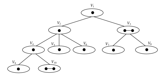
Figure 1: A cent-tree $T_{c}(Q)$ of a QT-graph on 12 vertices.

We next form the submatrix $B$ of the complement spanning-tree matrix $A$ for the graph $K_{n}-Q$ based on the structure of the cent-tree $T_{c}(Q)$, as well as on the $st$-partition of $T_{c}(Q)$.

Let $V^{\prime}_{1},V^{\prime}_{2},\ldots,V^{\prime}_{h}$ be the node sets of the $st$-partition of $T_{c}(Q)$. More precisely, the nodes of the $T_{c}(Q)$ are partitioned in the following sets:

$$V^{\prime}_{1} = V_{1},\ldots,V_{\ell},\ \ \ \ \ \ \ \ \ \ \ \ \ \ \ \ \ \ \ \ \ \ \ \ \ \ \ \ \ \ \ \ \ \ \ \ \ \ \ \ \ \ \ \ \ \ \ \ \ \ \ \ \ \ \ \ \ \ \ \ \ \ \ \ \ \ \ \ \ \ \ \ \ \ \ \ \ \ \ \ \ \ \ \ \ \ \ \ \ \ \ \ \ \ \$$

$$V^{\prime}_{2} = V_{\ell+1},\ldots,V_{s},\ \ \ \ \ \ \ \ \ \ \ \ \ \ \ \ \ \ \ \ \ \ \ \ \ \ \ \ \ \ \ \ \ \ \ \ \ \ \ \ \ \ \ \ \ \ \ \ \ \ \ \ \ \ \ \ \ \ \ \ \ \ \ \ \ \ \ \ \ \ \ \ \ \ \ \ \ \ \ \ \ \ \ \ \ \ \ \ \ \ \ \ \ \ \$$

$$\vdots$$

$$V^{\prime}_{h} = V_{k}.\ \ \ \ \ \ \ \ \ \ \ \ \ \ \ \ \ \ \ \ \ \ \ \ \ \ \ \ \ \ \ \ \ \ \ \ \ \ \ \ \ \ \ \ \ \ \ \ \ \ \ \ \ \ \ \ \ \ \ \ \ \ \ \ \ \ \ \ \ \ \ \ \ \ \ \ \ \ \ \ \ \ \ \ \ \ \ \ \ \ \ \ \ \ \$$

Then, we label the vertices of the graph $Q$ from $n-p+1$ to $n$ as follows: First, we label the vertices in $V_{1}$ from $(n-p)+1$ to $(n-p)+p_{1}$; next, we label the vertices in $V_{2}$ from $(n-p)+p_{1}+1$ to $(n-p)+p_{1}+p_{2}$; finally, we label the vertices in $V_{k}$.

Thus, based on the above labeling of the vertices of the QT-graph $Q$, we can easily construct the matrix $B$ of the graph $K_{n}-Q$; it is a $p\times p$ matrix and has the following form:

$B=\left[\begin{array}[]{ccccccccccc}M_{1}&&&&&&&&&&\\ &\ddots&&&&&&&&&\\ &&M_{\ell}&&&&&&&&\\ &&&M_{\ell+1}&&&&[b]_{j,i}&&&\\ &&&&\ddots&&&&&&\\ &&&&&M_{s}&&&&&\\ &&&&&&M_{s+1}&&&&\\ &&&[b]_{i,j}&&&&\ddots&&&\\ &&&&&&&&M_{r}&&\\ &&&&&&&&&\ddots&\\ &&&&&&&&&&M_{k}\end{array}\right]$, (2)

where $M_{i}$ is a $p_{i}\times p_{i}$ submatrix of the form

$M_{i}=\left[\begin{array}[]{cccc}a_{i}&b&\cdots&b\\ b&a_{i}&\cdots&b\\ \vdots&\vdots&\ddots&\vdots\\ b&b&\cdots&a_{i}\end{array}\right]$,

and the entries $[b]_{i,j}$ and $[b]_{j,i}$ of the off-diagonal positions $(i,j)$ and $(j,i)$, respectively, of matrix $B$ correspond to $p_{i}\times p_{j}$ and $p_{j}\times p_{i}$ submatrices with all their elements $b^{\prime}$s if node $V_{j}$ is a descendant of node $V_{i}$ in $T_{c}(Q)$ and zeros otherwise, $1\leq j\leq i\leq k$. Recall that $a_{i}=1-d_{i}b$, where $d_{i}$ is the degree of an arbitrary vertex in node $V_{i}$ of $T_{c}(Q)$, and $b=1/n$.

In order to compute the determinant of the matrix $B$ we first simplify the determinants of the matrices $M_{i}$, $1\leq i\leq k$. We multiply the last row of the matrix $M_{i}$ by $-1$ and add it to the first $p_{i}-1$ rows of the matrix $M_{i}$, $1\leq i\leq k$. Then we add the first $p_{i}-1$ columns of the matrix $M_{i}$ to the last column of the matrix $M_{i}$, $1\leq i\leq k$, and we obtain

$\det(M_{i})=\left|\begin{array}[]{cccc}a_{i}-b&&&\\ &a_{i}-b&&\\ &&\ddots&\\ b&b&&a_{i}-b+p_{i}b\end{array}\right|=(a_{i}-b)^{p_{i}-1}(a_{i}-(1-p_{i})b)$.

It now suffices to substitute the above value in the determinant of matrix $B$. We point out that after simplifying the determinant of matrices $M_{i}$ only the diagonal and the last row of each matrix $M_{i}$ have nonzero entries; the diagonal has nonzero entries since $d_{i}<n-1$. Thus, we have

$$\det(B)=\displaystyle\prod_{i=1}^{k}p_{i}({a_{i}-b})^{p_{i}-1}\det(D),$$ (3)

where

$D=\left[\begin{array}[]{ccccccccccc}\sigma_{1}&&&&&&&&&&\\ &\ddots&&&&&&&&&\\ &&\sigma_{\ell}&&&&&&&&\\ &&&\sigma_{\ell+1}&&&&(b)_{j,i}&&&\\ &&&&\ddots&&&&&&\\ &&&&&\sigma_{s}&&&&&\\ &&&&&&\sigma_{s+1}&&&&\\ &&&(b)_{i,j}&&&&\ddots&&&\\ &&&&&&&&\sigma_{r}&&\\ &&&&&&&&&\ddots&\\ &&&&&&&&&&\sigma_{k}\end{array}\right]$ (4)

is a $k\times k$ matrix with diagonal elements $\sigma_{i}=\frac{a_{i}-(1-p_{i})b}{p_{i}}$, $1\leq i\leq k$, and the entry $(b)_{i,j}$ of the off-diagonal position $(i,j)$ is $b$ if node $V_{j}$ is a descendant of node $V_{i}$ in $T_{c}(Q)$ and $0$ otherwise, $1\leq j\leq i\leq k$.

We observe that if we set $p_{i}=1$ in matrix $D$, $1\leq i\leq k$, then $D$ is equal to the submatrix $B$ of the graph $K_{n}-Q$, where $Q$ is a graph of a special type; it is a QT-graph on $k$ vertices possessing the property that each node of its cent-tree $T_{c}(Q)$ contains a single vertex; see Figure 2.

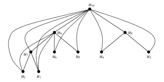
center

Figure 2: A QT-graph $Q$ on 10 vertices. Every node $V_{i}$ of the cent-tree $T_{c}(Q)$
contains exactly one vertex.

It is easy to see that, if we form the submatrix $B$ of the complement spanning-tree matrix $A$ of $K_{n}-Q$, where $Q$ is the QT-graph of Figure 2, using an appropriate vertex labeling, that is, $\ell_{2}=n-9,\ \ell_{1}=n-8,\ \ldots,\ \ell_{10}=n$, then we obtain $D=B$. The idea now is to transform the $k\times k$ matrix $D$ into a form similar to that of the $k\times k$ matrix $B$ of a tree $T$ on $k$ vertices; see Eq. (1) in Section 3. We proceed as follows:

We first apply the following operations to each row $i=1,2,\ldots,k$ of the matrix $D$:

• We find the minimum index $j$ such that $i<j\leq k$ and $D_{i,j}\neq 0$, and then

• we multiply the $j$th column by $-1$ and add it to the $\ell$th column, if $D_{i,\ell}=D_{i,j}$ and $j+1\leq\ell\leq k$.

Next, we apply similar operations to each column $j=1,2,\ldots,k$ of the matrix $D$:

• We find the minimum index $i$ such that $1\leq j<i$ and $D_{i,j}\neq 0$, and then

• we multiply the $i$th row by $-1$ and add it to the $\ell$th row, if $D_{\ell,j}=D_{i,j}$ and $i+1\leq\ell\leq k$.

Thus, we obtain

$\det(D)=\left|\begin{array}[]{ccccccccccc}a^{\prime}_{1}&&&&&&&&&&\\ &\ddots&&&&&&&&&\\ &&a^{\prime}_{\ell}&&&&(b^{\prime}_{j})_{j,i}&&&&\\ &&&a^{\prime}_{\ell+1}&&&&&&&\\ &&&&\ddots&&&&&&\\ &&&&&a^{\prime}_{s}&&&&&\\ &&(b^{\prime}_{j})_{i,j}&&&&a^{\prime}_{s+1}&&&&\\ &&&&&&&\ddots&&&\\ &&&&&&&&a^{\prime}_{r}&&\\ &&&&&&&&&\ddots&\\ &&&&&&&&&&a^{\prime}_{k}\end{array}\right|$,

where

$${}a^{\prime}_{i}=\begin{cases}\sigma_{i}&\text{if}\ V_{i}\ \text{is a leaf of}\ T_{c}(Q),\\ \\ \sigma_{i}+\displaystyle\sum_{j\in\text{ch}(i)\atop\ell+1\leq j\leq k}(\sigma_{j}-2b)&\text{otherwise},\end{cases}$$ (5)

and

$${}b^{\prime}_{i}=\begin{cases}b&\text{if }V_{i}\text{ is a leaf of }T_{c}(Q),\\ \\ b-\sigma_{i}&\text{otherwise}.\end{cases}$$ (6)

Note that the entry $(b^{\prime}_{j})_{i,j}$ in the off-diagonal position $(i,j)$ is $b^{\prime}_{j}$ if node $V_{j}$ is a descendant of node $V_{i}$ in $T_{c}(Q)$ and $0$ otherwise, $1\leq j\leq i\leq k$. Recall that $\sigma_{i}=\frac{a_{i}-(1-p_{i})b}{p_{i}}$; in the case where each node of the cent-tree $T_{c}(Q)$ contains a single vertex, we have $\sigma_{i}=a_{i}$ (in this case $p_{i}=1$, for every $i=1,2,\ldots,k$).

It is easy to see that the structure of the resulting $k\times k$ matrix $D$ is similar to that of the $k\times k$ matrix $B$ of a tree; see Eq. (1) in Section 3. Thus, for the computation of the determinant $\det(D)$, we can use similar techniques.

We next define the following function $\phi$ on the nodes on the cent-tree of a QT-graph $Q$:

$$\phi(i)=\begin{cases}a^{\prime}_{i}&\text{if }i\in V_{i}\text{ and }V_{i}\text{ is a leaf of }T_{c}(Q),\\ \\ a^{\prime}_{i}-\displaystyle\sum_{j\in\text{ch}(i)}{\frac{(b^{\prime}_{j})^{2}}{\phi(j)}}&\text{otherwise},\end{cases}$$

where $a^{\prime}_{i}$ and $b^{\prime}_{i}$ are defined in Eq. (5) and Eq. (6), respectively. We call the function $\phi$ the cent-function of the graph $Q$ or, equivalently, the cent-function of the cent-tree $T_{c}(Q)$; hereafter, we use $\phi_{i}$ to denote $\phi(i)$, $1\leq i\leq k$.

Following the same elimination scheme as that for the computation of the determinant of the matrix $B$ in Section 3, we obtain

$${}\det(D)=\displaystyle\prod_{i=1}^{k}\phi_{i}.$$ (7)

Thus, the results of this section are summarized in the following theorem.

Theorem 4.1. Let $Q$ be a quasi-threshold graph on $p$ vertices and let $V_{1},V_{2},\ldots,V_{k}$ be the nodes of the cent-tree of $Q$. Let $\phi$ be the cent-function of the graph $Q$. Then, the number of spanning trees of the graph $G=K_{n}-Q$ is equal to

$$\tau(G)=n^{n+k-p-2}\prod_{i=1}^{k}{p_{i}(n-d_{i}-1)^{p_{i}-1}\phi_{i}},$$

where $p_{i}$ is the number of vertices of the node $V_{i}$ and $d_{i}$ is the degree of an arbitrary vertex in node $V_{i}$, $1\leq i\leq k$.

Proof. As mentioned in Section 3, the complement spanning-tree matrix $A$ of a graph $K_{n}-Q$ can be represented by

$A=\left[\begin{array}[]{cc}I_{n-p}&\\ &B\\ \end{array}\right]$,

where the submatrix $B$ concerns those vertices of the graph $K_{n}-Q$ that have degree less than $n-1$; these vertices induce the graph ${\overline{Q\mkern 3.0mu}\mkern-3.0mu}{}$. Since $a_{i}=1-d_{i}b$ and $b=1/n$, from Eq. (3) we have

$$\det(B)=n^{k-p}\displaystyle\prod_{i=1}^{k}p_{i}(n-d_{i}-1)^{p_{i}-1}\det(D).$$

From the above equality and Eq. (7), we obtain

$$\det(B)=n^{k-p}\prod_{i=1}^{k}{p_{i}(n-d_{i}-1)^{p_{i}-1}\phi_{i}}.$$

The number of spanning trees $\tau(G)$ of the graph $G$ is equal to $n^{n-2}\det(A)$. Thus, since $\det(A)=\det(B)$, the theorem follows.   

Theorem 4.1 coupled with Theorem 3.1 implies a simple linear-time algorithm for computing the number of spanning trees of the graph $G=K_{n}-Q$, where $Q$ is a quasi-threshold graph on $p$ vertices, $p\leq n$ (see also Remark 3.1).

Remark 4.1. As mentioned in the introduction, the class of quasi-threshold graphs contains the class of c-split graphs (complete split graphs); recall that a graph is defined to be a c-split graph if there is a partition of its vertex set into a stable set $S$ and a complete set $K$ and every vertex in $S$ is adjacent to all the vertices in $K$ [6].

Thus, the cent-tree of a c-split graph $H$ consists of $|S|+1$ nodes $V_{1},V_{2},\ldots,V_{|S|+1}$ such that $V_{1}=K$ and the nodes $V_{2},V_{3},\ldots,V_{|S|+1}$ are children of the root $V_{1}$; each child contains exactly one vertex $u\in S$.

Let $H$ be a c-split graph on $p$ vertices and let $V(H)=K+S$ be the partition of its vertex set. Then, by Theorem 4.1, we obtain that the number of spanning trees of the graph $G=K_{n}-H$ is given by the following closed formula:

$\tau(G)=n^{n-p-1}(n-|K|)^{|S|-1}(n-p)^{|K|}$,

where $p=|K|+|S|$ and $p\leq n$.  $\Box$

5 Concluding Remarks

It is well known that the classes of quasi-threshold and threshold graphs are perfect graphs. Thus, it is reasonable to ask whether the complement spanning-tree matrix theorem can be efficiently used for deriving formulas, regarding the number of spanning trees, for other classes of perfect graphs [6].

It has been shown that the classes of perfect graphs, namely complement reducible graphs, or so-called cographs, and permutation graphs, have nice structural and algorithmic properties: a cograph admits a unique tree representation, up to isomorphism, called a cotree [11] (note that the class of cographs contain the classes of quasi-threshold and threshold graphs), while a permutation graph $G[\pi]$ can be transformed into a directed acyclic graph and, then, into a rooted tree by exploiting the inversion relation on the elements of the permutation $\pi$ [14].

Based on these properties, one can work towards the investigation whether the classes of cographs and permutation graphs belong to the family of graphs that admit formulas for the number of their spanning trees.

References

[1]
C. Berge, Graphs and Hypergraphs, North-Holland, Amsterdam,
1973.
[2]
T.J.N. Brown, R.B. Mallion, P. Pollak and A. Roth, Some methods
for counting the spanning trees in labelled molecular graphs,
examined in relation to certain fullerenes, Discrete Appl.
Math.67, 51–66, 1996.
[3]
K-L. Chung and W-M. Yan, On the number of spanning trees of a
multi-complete/star related graph, Inform. Process. Lett.76, 113–119, 2000.
[4]
C.J. Colbourn, The Combinatorics of Network Reliability,
Oxford University Press, New York, 1987.
[5]
B. Gilbert and W. Myrvold, Maximizing spanning trees in almost
complete graphs, Networks30, 23–30, 1997.
[6]
M.C. Golumbic, Algorithmic Graph Theory and Perfect Graphs,
Academic Press, New York, 1980.
[8]
P.L. Hammer and A.K. Kelmans, Laplacian spectra and spanning trees
of threshold graphs, Discrete Appl. Math.65,
255–273, 1996.
[9]
F. Harary, Graph Theory, Addison-Wesley, Reading, MA, 1969.
[10]
M. Kano and S.D. Nikolopoulos, On the structure of A-free graphs:
Part II, Tech. Report TR-25-99, Department of Computer Science,
University of Ioannina, 1999.
[11]
H. Lerchs, On cliques and kernels, Department of Computer Science,
University of Toronto, March 1971.
[12]
S. Ma, W.D. Wallis and J. Wu, Optimization problems on
quasi-threshold graphs, J. Comb. Inform. and Syst. Sciences.14, 105–110, 1989.
[13]
W. Myrvold, K.H. Cheung, L.B. Page, and J.E. Perry, Uniformly-most
reliable networks do not always exist, Networks21,
417–419, 1991.
[22]
W-M. Yan, W. Myrnold and K-L. Chung, A formula for the number of
spanning trees of a multi-star related graph, Inform.
Process. Lett.68, 295–298, 1998.
[23]
Y. Zhang, X. Yong and M.J. Golin, The number of spanning trees in
circulant graphs, Discrete Math.223, 337–350, 2000.
\captionstyle