Neural Network Ensembles: Evaluation of Aggregation Algorithms

Abstract

Ensembles of artificial neural networks show improved generalization capabilities that outperform those of single networks. However, for aggregation to be effective, the individual networks must be as accurate and diverse as possible. An important problem is, then, how to tune the aggregate members in order to have an optimal compromise between these two conflicting conditions. We present here an extensive evaluation of several algorithms for ensemble construction, including new proposals and comparing them with standard methods in the literature. We also discuss a potential problem with sequential aggregation algorithms: the non-frequent but damaging selection through their heuristics of particularly bad ensemble members. We introduce modified algorithms that cope with this problem by allowing individual weighting of aggregate members. Our algorithms and their weighted modifications are favorably tested against other methods in the literature, producing a sensible improvement in performance on most of the standard statistical databases used as benchmarks.

1 Introduction

For most regression and classification problems, combining the outputs of several predictors improves on the performance of a single generic one [22]. Formal support to this property is provided by the so-called bias/variance dilemma [12], based on a suitable decomposition of the prediction error. According to these ideas, good ensemble members must be both accurate and diverse, which poses the problem of generating a set of predictors with reasonably good individual performances and independently distributed predictions for the test points.

Diverse individual predictors can be obtained in several ways. These include: i) using different algorithms to learn from the data (classification and regression trees, artificial neural networks, support vector machines, etc.), ii) changing the internal structure of a given algorithm (for instance, number of nodes/depth in trees or architecture in neural networks), and iii) learning from different adequately-chosen subsets of the data set.

The probability of success in strategy iii), the most frequently used, is directly tied to the instability of the learning algorithm [2]. That is, the method must be very sensitive to small changes in the structure of the data and/or in the parameters defining the learning process. Again, classical examples in this sense are classification and regression trees and artificial neural networks (ANNs). In particular, in the case of ANNs the instability comes naturally from the inherent data and training process randomness, and also from the intrinsic non-identifiability of the model.

The combination of strong instability of the learning algorithm with the trade-off predictors’ diversity vs. good individual generalization capabilities requires an adequate selection of the ensemble members. Attempts to achieve a good compromise between the above mentioned properties include elaborations of two general techniques: bagging [2] and boosting [10]. These standard methods for ensemble construction follow two different strategies: Bagging (short for ’bootstrap aggregation’), and variants thereof, train independent predictors on bootstrap re-samples ${\emph{L}}_{n}$ ($n=1,M$) of the available data D, usually employing the unused examples ${\emph{V}}_{n}={\emph{D}}-{\emph{L}}_{n}$ for validation purposes. These predictors are then aggregated according to different rules (for instance, simple or weighted average). Boosting and its variants are stagewise procedures that, starting from a predictor trained on D, sequentially train new aggregate members on bootstrap re-samples drawn with modified probabilities. According to the general approach, each example in D is given a different chance to appear in a new training set by prioritizing patterns poorly learnt on previous stages. In the end, the predictions of the different members so generated are weighted with a decreasing function of the error each predictor makes on its training data.

For regression problems, on which we will focus here, boosting is still a construction area, where no algorithm has emerged yet as ’the’ proper way of implementing this technique [10, 7, 11, 1, 15, 23]. Consequently, bagging is the most common method for ANN aggregation. On the other hand, intermediate alternatives between bagging and boosting, which optimize directly the ensemble generalization performance instead of seeking for the best individual members, have not been much explored [21]. In this work we compare different strategies for ensemble construction, restricting ourselves to work in the regression setting and using ANNs as learning method. These restrictions are not essential; in principle, our analysis can be extended to classification problems and to other regression/classification methods. Furthermore, we will discuss stepwise algorithms to build the best aggregate after network training, thus incorporating the condition of optimal ensemble performance. Our main purpose is to establish rules as general as possible to build accurate regression aggregates. For this, we will

• discuss, in a unifying picture, several alternatives already proposed in the literature for the aggregation of ANNs,

• present a new algorithm that is optimal within this unified point of view,

• propose a simple weighting scheme of ensemble members that improves the aggregates’ generalization performances, and

• perform an extensive comparison of all these methods among themselves and with boosting techniques on several synthetic and real-world data sets.

The organization of this work is the following: In Section 2 we re-discuss several bagging-like methods proposed in the literature, considering them as different strategies for selecting the termination point of training processes for ensemble members. In this section we also present a new algorithm that is optimal from this point of view. In Section 3 we introduce the synthetic and real-world databases considered in this study, and describe the experimental settings used to learn from them. In Section 4 we obtain empirical evidence on the relative efficacy of all the methods discussed in Section 2 by applying them to these databases. Then, in Section 5 we present a modified, weighted version of the best algorithms and test their performances by comparison with the results in Section 4 and also against boosting and other techniques. Finally, in Section 6 we summarize the work done and the main results obtained, and draw some conclusions.

2 Ensemble Construction Algorithms

The simplest way of generating a regressor aggregate is bagging [2]. According to this method, from the data set D containing $N$ examples ($t,\mathbf{x}$) one generates bootstrap re-samples ${\emph{L}}_{n}$ ($n=1,M$) by drawing with replacement $N$ training patterns. Thus, each training set ${\emph{L}}_{n}$ will contain, on average, $0.63N$ different examples, some of them repeated one or more times [9]. The remaining $0.37N$ examples in ${\emph{V}}_{n}={\emph{D}}-{\emph{L}}_{n}$ are generally used for validation purposes in the regressor learning phase (backpropagation training of the ANN in our case). In this way one generates $M$ different members $f_{n}$ of the ensemble, whose outputs on a test point $\mathbf{x}$ are finally averaged to produce the aggregate prediction $\Phi({\mathbf{x}})=w_{1}f_{1}({\mathbf{x}})+...+w_{M}f_{M}({\mathbf{x}})$. The weights $w_{n}$ are usually taken equal to $1/M$ (simple averaging). Other options will be discussed in the next section. Notice that, according to this method, all the regressors are trained independently and their performances individually optimized using the “out-of-bag” data in ${\emph{V}}_{n}$. Then, although there is no fine-tuning of the ensemble members’ diversity, the method frequently improves largely on the average performance of the single regressors $f_{n}$.

Bagging can be viewed as a first stage in a sequence of increasingly more sophisticated algorithms for building a composite ANN regressor. To understand this, let’s consider first the situation in which a common validation subset V of the dataset D is kept unseen by all the networks during their training phases. Let’s also consider training to convergence $M$ ANNs on bootstrap re-samples ${\emph{L}}_{n}$ obtained now from ${\emph{L}}={\emph{D}}-{\emph{V}}$, saving the intermediate states $f_{n}(\tau)$ at each training epoch $\tau$ (i.e., $f_{n}(\tau)$ is the ANN model whose weights and biases take the values obtained at epoch $\tau$ of the training process). Building an ensemble is then translated to the task of selecting a combination of one state $f_{n}(\tau_{n}^{\mathrm{opt}})$ from each of the $M$ runs to create an optimal ensemble, that is, an ensemble with the smallest error on V. In this light, bagging solves the problem by choosing the state using only information on the given run ($\tau_{n}^{\mathrm{opt}}$ is the number of training epochs for which the validation error on V is minimum). In more advanced algorithms, the regressors are not optimized individually but as part of the aggregate. For ANNs, the simplest way of doing this is choosing a (common) optimal number of training epochs $\tau_{n}^{\mathrm{opt}}=\tau^{\mathrm{opt}}$ for all networks by optimizing the ensemble performance on V [18]:

$$\tau^{\mathrm{opt}}={\mathrm{argmin}}_{\tau}\sum_{(t,{\mathbf{x}})\in{\emph{V}}}[t-\Phi({\mathbf{x}},{\mathbf{w}}(\tau))]^{2}.$$

Here ${\mathbf{w}}(\tau)$ are the ANN internal parameters (weights and biases) at epoch $\tau$. Thus, instead of validating the ensemble members one by one to maximize their individual performances as in bagging, the algorithm selects a common optimal stopping point $\tau^{\mathrm{opt}}$ for all the networks in the ensemble. In practice, one finds that $\tau^{\mathrm{opt}}$ is in general larger than the individual stopping points found in bagging, i.e., some controlled degree of single network overfitting improves the aggregate’s performance. In the following we will refer to this algorithm as “Epoch”.

The above described strategy can be further pushed on by selecting not a single optimal $\tau^{\mathrm{opt}}$ for all networks but independent $\tau^{\mathrm{opt}}_{n}$ for each network in the ensemble. This requires minimizing

$$E({\vec{\tau}})=\sum_{(t,{\mathbf{x}})\in{\emph{V}}}[t-\Phi({\mathbf{x}},{\mathbf{w}}({\vec{\tau}}))]^{2}$$

as a function of the set of training epochs ${\vec{\tau}}=\{\tau_{n};n=1,M\}$ for all networks. This can be accomplished, for instance, by using simulated annealing in ${\vec{\tau}}$-space. That is, starting from networks trained ${\vec{\tau}}_{0}$ epochs, we randomly change $\tau_{0n}$ and check whether the ensemble generalization error (2) increases or decreases when network $n$ is trained up to $\tau_{0n}+\Delta\tau$. As usual, we accept the move with probability 1 when $E({\vec{\tau}})$ decreases, and with probability

$${\frac{\exp\{-\beta[E({\vec{\tau}})-E({\vec{\tau}}_{0})]\}}{1+\exp\{-\beta[E({\vec{\tau}})-E({\vec{\tau}}_{0})]\}}}$$

when $E({\vec{\tau}})$ increases. This is repeated many times considering different networks $n$ (chosen either at random or sequentially), while the annealing parameter $\beta$ is conveniently increased at each step; the algorithm runs until $E({\vec{\tau}})$ settles in a deep local minimum. In practice we have taken $\Delta\tau=r\tau^{\mathrm{max}}/20$, where $\tau^{\mathrm{max}}$ is the maximum number of training epochs and $r$ is a random number in the interval $[-1,1]$. The annealing temperature was decreased according to $\beta^{-1}=0.995^{q}E({\vec{\tau_{0}}})/2$, where $q$ is the annealing step. We point out that the minimization problem is simple enough not to depend critically on these choices. As far as we know, this algorithm —which we will call “SimAnn”— has not been previously discussed in the literature and constitutes one of the main contributions of this work. Notice that for its implementation, as well as for the simplest implementation of Epoch, one is forced to store all the intermediate networks $f_{n}[{\mathbf{w}}(\tau)]$. However, given the large storage capacity in computers nowadays, in most applications this requirement is not severe.

In the common situation of scarcity of data, the need to keep an independent validation set V is a serious drawback that limits the efficacy of the methods discussed above. An alternative approach is to resort to the out-of-bag patterns $(t_{p},{\mathbf{x}}_{p})\in{\emph{V}}_{n}$ unseen by network $f_{n}$, and optimize with respect to the number of training epochs the error

$$E({\vec{\tau}})=\sum_{p=1}^{N}[t_{p}-\Phi_{p}({\mathbf{x}}_{p},{\mathbf{w}}({\vec{\tau}}))]^{2}.$$ (1)

Here $\Phi_{p}({\mathbf{x}}_{p},{\mathbf{w}}(\vec{\tau}))=\sum_{n=1,M}w_{pn}f_{n}[{\mathbf{x}}_{p},{\mathbf{w}}(\vec{\tau})]$ is the aggregate regressor built with those networks that have not seen pattern $(t_{p},{\mathbf{x}}_{p})$ in their training phase, i.e.

$$w_{pn}=\frac{\gamma_{pn}}{\sum_{n}\gamma_{pn}},$$

where $\gamma_{pn}=1$ if $(t_{p},{\mathbf{x}}_{p})\in{\emph{V}}_{n}$ and 0 otherwise. Notice that the validation procedure generated by Eq. (1) amounts to effectively optimizing the performances of several subsets of the $M$ trained ANNs, each subset including on average $0.37M$ networks. The advantage is that, like in the description of bagging at the beginning of this section, no sub-utilization of data for validation purposes is necessary.

The above described strategy can be slightly simplified by selecting independent $\tau^{\mathrm{opt}}_{n}$ for each network in the ensemble. This is the proposal of the so-called NeuralBAG algorithm [5], which chooses

$$\tau^{\mathrm{opt}}_{n}={\mathrm{argmin}}_{\tau}\sum_{(t_{p},{\mathbf{x}}_{p})\in{\emph{V}}_{n}}[t_{p}-\Phi_{p}({\mathbf{x}}_{p},{\mathbf{w}}(\tau))]^{2}$$ (2)

This is a rather ad hoc criterion: notice that in (2) the networks $f_{m}$ with $m\neq n$ are trained up to $\tau^{\mathrm{opt}}_{n}$, but they are effectively trained $\tau^{\mathrm{opt}}_{m}$ epochs in the final ensemble. Nevertheless, judging from the reported results [5], it seems to be effective in practice.

All the strategies for ANN aggregation discussed so far minimize some particular error function in a global way. A different approach is to adapt the typical hill-climbing search method to this problem. In a previous work [13] we proposed a simple way of generating a ANN ensemble through the sequential aggregation of individual predictors, where the learning process of a new ensemble member is validated by the previous-stage aggregate prediction performance. That is, the early-stopping method is applied by monitoring the generalization capability on ${\emph{V}}_{\mathrm{n+1}}$ of the $n$-stage aggregate predictor plus the $n+1$ network being currently trained. In this way we retain the simplicity of independent network training and only the validation process becomes slightly more involved, leading again to a controlled overtraining (“late-stopping”) of the individual networks. Notice that, despite the stepwise characteristic of this algorithm (here called SECA, for Stepwise Ensemble Construction Algorithm), it can be implemented after the parallel training of networks if desirable. Alternatively, if implemented sequentially it avoids completely the burden of storing networks at intermediate training times like in the algorithms described above.

For the sake of completeness, we summarize the implementation of SECA as follows:

Step 1: Generate a training set ${\emph{L}}_{1}$ by a bootstrap re-sample from dataset D, and a validation set ${\emph{V}}_{1}={\emph{D}}-{\emph{L}}_{1}$ by collecting all instances in D that are not included in ${\emph{L}}_{1}$. Produce a model $f_{1}$ by training a network on ${\emph{L}}_{1}$ until a minimum $e_{f}({\emph{V}}_{1})$ of the generalization error on ${\emph{V}}_{1}$ is reached.

Step 2: Generate new training and validation sets ${\emph{L}}_{2}$ and ${\emph{V}}_{2}$ respectively, using the procedure described in Step 1. Produce a model $f_{2}$ training a network until the generalization error on ${\emph{V}}_{2}$ of the aggregate predictor $\Phi_{2}=(f_{1}+f_{2})/2$ reaches a minimum $e_{\Phi}({\emph{V}}_{2})$. In this step the parameters of model $f_{1}$ are kept constant and the model $f_{2}$ is trained with the usual (quadratic) cost function on ${\emph{L}}_{2}$.

Step 3: Iterate the process until a number $M$ of models is produced. A suitable $M$ can be estimated from the behavior of $e_{\Phi}({\emph{V}}_{n})$ as a function of $n$, since this error will stabilize when adding more networks to the aggregate becomes useless.

In this algorithm the individual networks are directly trained with a late-stopping method based on the current ensemble generalization performance. The method seems to reduce the aggregate generalization error without paying much attention to whether this improvement is related to enhancing the members’ diversity or not. However, one can see [13] that it actually finds diverse models to reduce the ensemble error by looking, at every stage, for a new model anticorrelated with the current ensemble. Notice that SECA can be also implemented using an external validation set V, in which case all the bootstrap complements ${\emph{V}}_{n}$ are replaced by this fixed set.

All the above described methods constitute a chain of increasingly optimized algorithms for ensemble building, starting from the simplest Bagging idea of optimizing networks independently to SimAnn, which should produce the “optimal” ensemble (i.e., the ensemble with the minimum validation error 1). Let’s consider a simple analysis of the computational cost involved in the implementation of these algorithms. Once the $M$ ANNs have been independently trained and $T$ networks saved along each training evolution, which is common to all the algorithms, Bagging requires a computational time $t\sim M\times T$ to select the best combination (essentially, the evaluation of the $T$ ANN’s validation errors for each of the $M$ networks to find the corresponding minima). Epoch requires exactly the same computational effort to find the (common) optimal stopping point for all networks. NeuralBag uses, instead, $t\sim M^{2}\times T$ evaluations to find the best aggregate. Finally, SECA and SimAnn require ${\frac{(M+1)}{2}}\times M\times T$ and $p\times M\times T$ network evaluations, respectively. Here we have written the number of simulated annealing steps $N_{\mathrm{sa}}=pT$, with $p$ an arbitrary integer, to facilitate the comparison. In the following we will take $p\sim M$ to have a fair comparison between NeuralBag, SECA and SimAnn. Notice, however, that the major demand from a computational point of view is the ANN training and not the network selection to build the ensemble. In practice, in the algorithms’ evaluations in Section 4 and 5 we have taken $M=20$, $T=200$ and $p=15$, with all the networks trained a maximum of $10T$ to $100T$ epochs, depending on the database.

As mentioned in the Introduction, a completely different strategy for building composite regression/classification machines is boosting. For classification problems, its main difference with bagging is the use of modified probabilities to re-sample the training sets ${\emph{L}}_{n}$. At stage $n$, the weights associated to examples in D are larger for those examples poorly learnt in previous stages, so that they eventually appear several times in ${\emph{L}}_{n}$. In this way, the new predictor $f_{n}$ trained on ${\emph{L}}_{n}$ specializes on these hard examples. Finally, the inclusion of $f_{n}$ in the ensemble with a suitably-chosen weight allows the exponential decrease with boosting rounds $n$ of the ensemble’s training error on the whole dataset D. Notice that, in addition to the above mentioned modification of re-sampling probabilities, other differences with bagging are: i) boosting is essentially a stage-wise approach, which requires a sequential training of the aggregate members $f_{n}$, and ii) in the final ensemble these members are weighted according to their performances on the respective training sets ${\emph{L}}_{n}$ (using a decreasing function of the training error). A further consideration of this last characteristic will be done in Section 4, where we discuss a weighting scheme for bagged regressors alternative to the simple average considered in this section.

While boosting is, as explained above, a well defined procedure in the classification setting, for regression problems there are several ways of implementing its basic ideas. Unfortunately, none of them has yet emerged as “the” proper way of boosting regressors. Without the intention of exhausting all the proposed implementations, we can distinguish two boosting strategies for solving regression problems: i) by forward stage-wise additive modelling, which modifies the target values to effectively fit residual errors[11, 15, 8], and ii) by reducing the regression problem to classification and essentially changing example weights to emphasize those which were poorly learnt on previous stages of the fitting process [10, 20, 7, 23]. In order to compare with the bagging-like algorithms described above, in this work we will implement the boosting techniques from [11] and [7] as examples of these two different strategies.

In Sections 4 and 5 we will show how all the heuristic algorithms described in this section work on real and synthetic data. This will provide a fairly extensive comparison of the already known methods and will test the new SimAnn algorithm against all the other methods. In the next section we briefly describe the databases and experimental settings considered for this comparison.

3 Benchmark Databases and Experimental Settings

We have evaluated the algorithms described in the previous section by applying them to several benchmark databases: the synthetic Friedman #1, 2, 3 data sets and chaotic Ikeda map, and the real-world Abalone, Boston Housing, Ozone and Servo data sets. In the cases of the Friedman data sets we can control the (additive) noise level, which allows us to investigate its influence on the different algorithm’s performances. We present the results for the Ikeda map together with those of real-world sets because the level of noise in this problem is fixed by its intrinsic dynamics. In addition, at the end of next section we will present results on the Mackey-Glass equation, which allows a more general comparison with other regression methods in the literature previously applied to this problem [16, 19].

In the following we give brief descriptions of the databases and the ANN architectures used. In all cases, the number of hidden units $h$ have been selected by trial and error, using a validation set and looking for the minimum generalization error on this set as a function of $h$. Once the network architecture was chosen, it was kept the same during all the calculations. Notice that this is not a particularly important point, since we want to compare the efficacy of different aggregation methods and all of them use the same trained networks.

• Friedman #1

  The Friedman #1 synthetic data set corresponds to training vectors with 10 input and one output variables generated according to

  $$t=10\sin(x_{1}x_{2})+20(x_{3}-0.5)^{2}+10x_{4}+5x_{5}+\varepsilon,$$ (3)

  where $\varepsilon$ is Gaussian noise and $x_{1},\ldots x_{10}$ are uniformly distributed over the interval $[0,1]$. Notice that $x_{6},\dots x_{10}$ do not enter in the definition of $t$ and are only included to check the prediction method’s ability to ignore these inputs. In order to explore the algorithm’s performances in different situations we considered different noise levels and training set lengths. The Gaussian noise component was alternatively set to: $\varepsilon=0$ (No noise, labeled “free”), $\varepsilon$ with normal distribution ${\emph{N}}(\mu=0,\sigma=1)$ (low noise), and $\varepsilon$ with normal distribution ${\emph{N}}(\mu=0,\sigma=2))$ (high noise). We generated 1200 sample vectors for each noise level and these data sets were randomly split in training and test sets. The training sets D had alternatively 50, 100 and 200 patterns, while the test set contained always 1000 examples. We considered ANNs with 10:$h$:1 architectures, with the number of hidden units $h=6,10$ and 15 for increasing number of patterns in the training set.
  

• Friedman #2

  Friedman #2 has four independent variables and the target data are generated according to

  $$y=x_{1}^{2}+\sqrt{x_{2}x_{3}-(x_{2}x_{4})^{-2}}+\varepsilon$$

  where the zero-mean, normal noise is adjusted to give noise-to-signal power ratios of 0 (no noise), 1:9 (low noise) and 1:3 (high noise). The variables $x_{i}$ are uniformly distributed in the ranges

  $$0<x_{1}<100,\ \ \ 20<\frac{x_{2}}{2\pi}<280,\ \ \ 0<x_{3}<1,\ \ \ 1<x_{4}<11$$

  The training sets contained 20, 50 and 100 patterns, and the test set had always 1000 patterns. We considered 4:$h$:1 ANNs, with $h=4,6$ and 8 according to the training set length.
  

• Friedman #3

  Friedman #3 has also four independent variables distributed as above but the target data are generated as

  $$y=\tan^{-1}\left[{\frac{x_{2}x_{3}-(x_{2}x_{4})^{-2}}{x_{1}}}\right]+\varepsilon$$

  The noise-to-signal ratios were chosen as before, but in this case the training sets contained 100, 200 and 400 patterns. Accordingly, we considered $h=6,8$ and 12. As in the previous cases, the test sets had always 1000 patterns.
  

• Abalone

  The age of abalone is determined by cutting the shell through the cone, staining it, and counting the number of rings through a microscope. To avoid this boring task, other measurements easier to obtain are used to predict the age. Here we considered the data set that can be downloaded from the UCI Machine Learning Repository (ftp to ics.uci.edu/pub/machine-learning-databases), containing 8 attributes and 4177 examples without missing values. Of these, 1045 patterns were used for testing and 3132 for training (for all real-world problems considered, the data set splitting in learning and test sets was chosen following [3]). The ANNs used to learn from this set had a 8:5:1 architecture.
  

• Boston Housing

  This data set consists of 506 training vectors, with 11 input variables and one target output. The inputs are mainly socioeconomic information from census tracts on the greater Boston area and the output is the median housing price in the tract. These data can also be downloaded from the UCI Machine Learning Repository.

  Here we considered 450 training examples and 56 data points for the test set. The ANNs used had a 11:5:1 architecture.
  

• Ozone

  The Ozone data correspond to meteorological information (humidity, temperature, etc.) related to the maximum daily ozone (regression target) at a location in Los Angeles area. Removing missing values one is left with 330 training vectors, containing 8 inputs and one target output in each one. The data set can be downloaded by ftp (to ftp.stat.berkeley.edu/pub/users/breiman) from the Department of Statistics, University of California at Berkeley.

  We considered ANNs with 8:5:1 architectures and performed a (random) splitting of the data in training and test sets containing, respectively, 295 and 35 patterns.
  

• Servo

  The servo data cover an extremely non-linear phenomenon –predicting the rise time of a servomechanism in terms of two (continuous) gain settings and two (discrete) choices of mechanical linkages. The set contains 167 instances and can be downloaded from the UCI Machine Learning Repository.

  We considered 4:15:1 ANNs, using 150 examples for training and 17 examples for testing purposes.
  

• Ikeda

  The Ikeda laser map [14], which describes instabilities in the transmitted light by a ring cavity system, is given by the real part of the complex iterates

  $$z_{n+1}=1+0.9z_{n}\exp\left[0.4i-{\frac{6i}{(1+|z_{n}|^{2})}}\right].$$

  Here we have generated 1100 iterates, using 100 in the training set and 1000 for testing purposes.

  After some preliminary investigations, we chose an embedding dimension 5 for this map and considered ANNs with a 5:10:1 architecture.

For each one of these databases we trained $M=20$ independent networks, storing $T=200$ intermediate weights and biases ${\mathbf{w}}({\vec{\tau}})$ on long training experiments until convergence ($10T$ to $100T$ epochs, depending on the database). We considered this number of networks after checking on preliminary evaluations that there were no sensible performance improvements with bigger ensembles. With these 20 ANNs we implemented the different bagging-like ensemble construction algorithms, changing the training stopping points of individual networks according to the criteria discussed in the previous section. We did this for the following two different validation scenarios:

• Keeping an external validation set V, randomly selected from the data set D, and training the 20 ANNs on different bootstrap re-samples of ${\emph{L}}={\emph{D}}-{\emph{V}}$. Here we considered two partitions of D: 20/80% and 37/63% (following the bootstrap proportion), where in each case the first number indicates the fraction of data points in V. For this case only the bagging-like algorithms discussed in the previous section were considered.

• Validating the training process directly with the out-of-bag data, as explained in the previous section. This procedure makes full use of the available data, and in general should produce better results than the previous situation. In this case we tested bagging-like techniques and also boosted ANNs according to the Friedman [11] and Drucker [7] algorithms, considering a maximum of 20 boosting rounds for comparison.

The results given in the following section correspond to an average over 50 independent runs of the above-described procedures, without discarding any anomalous case (for Boston, Ozone and Servo databases we averaged over 100 experiments because the smaller test sets allow larger sample fluctuations). We will not indicate the variance of average errors, since these deviations only characterize the dispersion in performances due to different realizations of training and test sets. They have no direct relevance in comparing the average performances of different methods (in each run all the algorithms use the same 20 networks). This procedure guarantees that differences in the final ensemble performances are only due to the aggregation methods and/or validation settings.

Finally, at the end of Section 5 we compare the best performing algorithms here considered with several other methods in the literature. For this comparison we use the chaotic Mackey-Glass time series:

• Mackey-Glass

  The Mackey-Glass time-delay differential equation is a model for blood cell regulation. It is defined by

  $${\frac{dx(t)}{dt}}={\frac{0.2x(t-\tau)}{1+x^{10}(t-\tau)}}-0.1x(t)$$ (4)

  When $x(0)=1.2$ and $\tau=17$, we have a non-periodic and non-convergent time series that is very sensitive to initial conditions (we assume $x(t)=0$ when $t<0$).

  In order to compare with the results in [16] and [19], we have downloaded the database used by these authors and considered, like in these works, an embedding dimension $d=6$ and 1194 patterns for training and 1000 patterns for testing purposes. For this problem we took $h=40$.

4 Evaluation Results

The results quoted below are given in terms of the normalized mean-squared test error:

$$NMSE_{\emph{T}}={\frac{MSE_{\emph{T}}}{\sigma^{2}_{\emph{D}}}},$$ (5)

defined as the mean-squared error on the test set T divided by the variance of the total data set D. According to this definition, $NMSE\simeq 1$ for a constant predictor equal to the data average and 0 for a perfect one. Then, its value allows to appraise both the predictor’s performance and the relative complexity of the different regression tasks. Notice that, as indicated in the table captions, the results are given in units of $10^{-2}$, so that all the errors are much smaller than 1 and, consequently, the predictions much better than the trivial data average.

In Tables 1a and 1b we present results for synthetic and real databases respectively, in the situation in which an external validation set containing 20% of the data is used. Tables 2a and 2b correspond to the same case but with 37% of validation data. As mentioned in the previous section, here only bagging-like algorithms are compared. Tables 3a and 3b present the corresponding results for all bagging-like algorithms and out-of-bag validation (no hold out data).

First, for external validation, the experiments indicate that Epoch performs better than Bagging in only 2 of the 27 cases corresponding to synthetic databases (Friedman #1,2 and 3, Tables 1a and 2a), and in 2 or none out of 5 cases for the real-world databases (Tables 1b and 2b), depending on the validation set size. This poor performance becomes slightly better for out-of-bag validation (9/27, Table 3a, and 3/5, Table 3b, respectively). Consequently, we do not find any advantage in using this algorithm instead of Bagging. Something similar happens with NeuralBag, which, in spite of the good results presented in [5], in our experiments only improves on Bagging in roughly half the cases. On the contrary, both SECA and SimAnn are clearly better than Bagging: on average, both methods outperform Bagging approximately in 21 of the 27 Friedman problems and in all but one case for real databases, independently of the validation used.

Considering all the methods together, Table 1a shows that, for the 27 learning problems associated to the Friedman synthetic data, in 22 cases the best method is either SECA or the network selection via simulated annealing (SimAnn). This pattern is confirmed by the results in Table 2a, where SECA and SimAnn are again the best performers in 22 of the 27 cases. For the real-world databases these two methods outperform the other bagging-like algorithms in all cases (see Tables 1b and 2b), with a particularly good performance of SimAnn. For out-of-bag validation, Table 3a shows that, consistently with the previous results, in 19 of the 27 experimental situations SECA and SimmAnn are the best performers. We stress, however, the good performance of Epoch on Friedman #2 data set, particularly for noise-free data. For the real-world databases, Table 3b shows that SECA and SimAnn produced the best results in all but one (Servo) of the regression problems investigated. All these results obey the expected behaviors with noise level and data set length. Furthermore, for the synthetic Friedman problems in general the test error is larger when more data are held out for validation, although this not the case for the real-world Abalone, Boston and Ozone datasets. Moreover, for bagged regressors, independently of the method used to ensemble them, in all cases the out-of-bag validation is more efficient than keeping an external set, in agreement with other works in the literature[4]. Notice, however, that this last observation is not valid in the noisy Friedman #2 and Servo problems for a single ANN.

In the case of out-of-bag validation, we have performed a paired $t$-test to check whether SECA and SimAnn significantly outperform Bagging. Following the procedure in [6], we considered a binary variable that assumes a value of 1 when SECA/SimAnn is better than Bagging and 0 otherwise. If the average of this variable differs from 0.5 and this difference is statistically significant, we can affirm that one of the methods is better than the other. The results of the $t$-test are given in Tables 4a and 4b. For Friedman #1, SECA and SimAnn are better than Bagging in all cases; for Friedman #2 there are no clear differences between the methods, and for Friedman #3 SECA and SimAnn are significantly better than Bagging except for high noise and few patterns in the training set. For the real-world databases, SECA and SimAnn are always better than Bagging, with more than 95% of statistical significance in several cases. These results are in complete agreement with the NMSE comparison in Tables 1-3.

4.1 Accuracy vs. Diversity

In order to gain some insight into SECA and SimAnn’s behaviors that might explain the good performances shown in Tables 1-4, we have investigated the standard bias-variance decomposition of the generalization error[12].

Consider general regression problems where vectors $\mathbf{x}$ of predictor variables are obtained from some distribution $P(\mathbf{x)}$ and regression targets $t$ are generated according to $t=f(\mathbf{x})+\varepsilon$. Here $f$ is the true regression function and $\varepsilon$ is random noise with zero mean. If we estimate $f$ learning from a data set L and obtain a model $f_{\emph{L}}$, the (quadratic) generalization error on a test point $(t,\mathbf{x})$ averaged over all possible realizations of L (with respect to $P$ and noise $\varepsilon$) can be decomposed as:

$$\mathrm{E}[(t-f_{{\emph{L}}}(\mathbf{x}))^{2}|{\emph{L}}] = \mathrm{E}[\varepsilon^{2}|\varepsilon]$$

$$+ (\mathrm{E}[f_{\emph{L}}(\mathbf{x})|{\emph{L}}]-f(\mathbf{x}))^{2}+\mathrm{E}[(f_{\emph{L}}(\mathbf{x})-\mathrm{E}[f_{\emph{L}}(\mathbf{x})|{\emph{L}}])^{2}|{\emph{L}}]$$

The first term on the right-hand side is simply the noise variance $\sigma_{\varepsilon}^{2}$; the second and third terms are, respectively, the squared bias and variance of the estimation method.

From the point of view of a single estimator $f_{\emph{L}}$, we can interpret this equation by saying that a good method should be not biased and have as little variance as possible between different realizations. There are learning methods (for instance, ANNs) for which the first condition is reasonably well met but the second one is not satisfied since, for small changes or even with no changes at all in L, different learning experiments lead to distinct predictors $f_{\emph{L}}$ (unstable learning methods). A way to take advantage of this apparent weakness of these methods is to make an aggregate of them.

If we rewrite the error decomposition in the form:

$$\mathrm{E}[(t-\mathrm{E}[f_{\emph{L}}(\mathbf{x})|{\emph{L}}])^{2}|{\emph{L}}]\equiv\mathrm{Bias}^{2}+\sigma_{\varepsilon}^{2}=\mathrm{MeanError}-\mathrm{Variance},$$ (7)

we can reinterpret this equation in the following way: using the ensemble average $\Phi\equiv\mathrm{E}[f_{\emph{L}}|{\emph{L}}]$ as estimator, the generalization error can be reduced if we produce fairly accurate models $f_{\emph{L}}$ (small MeanError) that output diverse predictions for each test point (large Variance). Of course, there is a trade-off between these two conditions, but finding a good compromise between the regressors’ mean accuracy ($\equiv 1/\textrm{MeanError}$) and diversity ($\equiv\textrm{Variance}$) seems particularly feasible for largely unstable methods like ANNs.

For the results shown in Table 2a we have estimated separately the accuracy and diversity components of the error according to 7. In Table 5 we present the results obtained; for easier comparison, we give them normalized by the mean accuracy and diversity of the bagging ensemble members. As expected, bagging produces the most accurate but less diverse predictors; instead, the other aggregation methods resign some accuracy to gain diversity. More interestingly, we see that, despite the similar performance of SECA and SimAnn in Table 2a, these aggregation methods select very different ensemble members. In particular, SimAnn seeks mainly for diverse predictors although they are not very accurate while SECA introduces diversity in a more balanced way with accuracy. Epoch strategy is in general intermediate between these two methods but not effective enough to outperform them.

5 Weighting Ensemble Members

In the previous section we evaluated several ensemble construction algorithms that essentially differ in the way they select the particular stopping points for independently-trained ANNs. The final aggregate prediction on a test point is simply the mean of the individual predictions, without weighting the outputs of the ensemble members ($w_{n}=1/M$, $n=1,M$). This is not particularly wise for SECA, since some of these members may have poor generalization capabilities. SECA is a stepwise optimization technique, and a known problem with these heuristics is that during the optimization process they cannot review the choices made in the past. Figure 1 shows a typical example of the problem one can find for a given realization of the Friedman #1 data set. Open circles represent the evolution of training and test errors during the construction of the ensemble using SECA. In this example, the fourth added network clearly deteriorates the ensemble performance, and this effect cannot be compensated by the addition of more networks. Obviously, it also influences the selection of the following ensemble members.

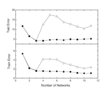
Figure 1: Evolution of training and test errors during the ensemble construction, in arbitrary units. Open circles correspond to SECA; dots indicate the same evolution when ensemble members are weighted according to W-SECA.

In a previous work [17] we explored a possible way to cope with this problem, using a slightly different SECA algorithm that only accepts networks that improve the ensemble performance. Unfortunately, new results showed that this algorithm also produces some overfitting, being unable to clearly outperform bagging on small and noisy data sets. A possible intermediate solution is weighting the ensemble members, instead of rejecting them if they do not improve the overall ensemble performance. This allows us to reduce the influence of bad choices made in the past by simply giving smaller weights to troublesome networks. Then, following general ideas from boosting, we propose to modify the algorithm so that the output of the ensemble at the $m$-th stage becomes

$$\Phi_{m}({\mathbf{x}})=\sum_{n=1}^{m}w_{n}f_{n}({\mathbf{x}}),$$ (8)

where $w_{n}$ is a decreasing function of $e_{n}$, the MSE of the $n$-th member over D; i.e., we weight each ensemble member according to its individual performance on the whole dataset. This is the way in which boosting reduces the importance of overfitted members in the final ensemble. In practice we have explored two different weighting functions:

$$w_{i}=\frac{e_{i}^{-\alpha}}{\sum_{j}e_{j}^{-\alpha}},\ \ \ w_{i}=\frac{\exp(-\alpha e_{i})}{\sum_{j}\exp(-\alpha e_{j})}.$$ (9)

Figure 2 shows the results obtained with SECA on Friedman #1 for both weighting schemes. As we can see, for small to intermediate values of $\alpha$ weighting produces better results than simply averaging the individual predictions. For large values of $\alpha$ some overfitting is observed, since only a few particular networks effectively contribute to the ensemble. As expected, this is more acute for exponential weighting, but there are no other major differences between both laws. On the other hand, the smaller the noise the larger one can take $\alpha$ before overfitting is observed. We have also considered Friedman #2 and 3 data sets, and the behavior in Figure 2 is representative of the general trend.

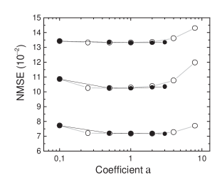
Figure 2: Normalized mean-squared test error NMSE as a function of the weighting coefficient $\alpha$ for Friedman #1 data sets (From top to bottom: high noise, low noise and noise-free data). Open circles (dots) correspond to exponential (potential) weighting.

In Figure 1 we have included the results of weighting SECA using the power law with $\alpha=2$ (this algorithm will be called W-SECA) for the case discussed above. The problematic fourth network is given a small weight, and is practically ignored by the ensemble.

We have performed the $t$-test described before to establish whether the performance obtained with W-SECA is significantly better than that of SECA. To have a fair evaluation of the algorithm just described we used the same ANNs considered in the previous section. Tables 6a and 6b show the corresponding results, which indicate that W-SECA outperforms SECA with statistical significance in practically all situations studied.

We have also applied the weighting scheme to Bagging and SimAnn to investigate if the effective elimination of some bad ensemble members (by giving them small weights) has also impact on these algorithms. One question to answer here is: Will this improvement wash out the differences observed in Tables 1-4 between the different algorithms? In order to have a fair evaluation of the algorithms we used the same ANNs considered in the previous section. The results obtained are collected in Tables 7a and 7b.

These tables show that for the 27 regression problems corresponding to Friedman #1, 2 and 3 data sets, W-SECA and W-SimAnn outperform Bagging in 21 and 22 cases respectively. Moreover, for the real-world databases and Ikeda map, W-SimAnn is always better than W-Bagging, and W-SECA looses only on the Servo database against W-Bagging. That is, although weighting is in general beneficial for all algorithms, the member selection strategy is still important to obtain good performances. This is also supported by the results of paired $t$-tests between W-SECA and W-SimAnn against W-Bagging (see Tables 8a and 8b).

It is also of interest to mention that the weighted algorithms outperform non-weighted ones in 26 out of the 32 cases investigated (compare best results in Tables 3 and 7). From the remaining 6 cases, 4 correspond to high noise-scarce data situations. Notice also that in these cases the best performers are SECA and SimAnn. Finally, we stress that from the 32 problems considered, W-Bagging performs better than Bagging in 27 cases, W-SimAnn performs better than SimAnn in 29 cases, and W-SECA performs better than SECA in 31 cases. We remark the important improvements for SECA, which were expected according to the above discussion in connection with Figure 1.

In Tables 7a and 7b we also present results obtained with the boosting algorithms proposed in [7] (“D-Boosting”) and [11] (“F-Boosting”) for comparison. For these algorithms we used a maximum of 20 boosting rounds, which should produce a fair test considering the 20 ANNs ensembled in the bagging-like methods. Notice that for the 27 Friedman datasets the boosting algorithms perform better than W-SECA and W-SimAnn only in three cases, and in these few cases the “D-Boosting” implementation is always the best performer. For the real-world databases and Ikeda map this implementation and W-SimAnn are the top performers.

As a final investigation on W-SECA and W-SimAnn, we have considered the Mackey-Glass problem. This allows us to make a comparison with seven other regression methods based on Support Vector Machines (SVM) and regularized boosting using Radial Basis Function (RBF) networks, as described in [16] and [19]. Following these works, we introduced three levels of uniform noise to the training set, with signal-to-noise ratios of 6.2%, 12.4% and 18.6% respectively, and Gaussian noise with signal-to-noise ratios of 22.15% and 44.30% respectively. The test set is kept noiseless to measure the true prediction error. As mentioned in Section 4, to have a fair comparison all the experimental settings (training and test set lengths, embedding dimension, etc.) are the same as in [16] and [19]. Table 9 presents the corresponding results, which show that W-SECA and W-SimAnn are among the top performers in most cases. We stress that they perform worse than SVM methods only for the largest Gaussian noise case (we are disregarding the CG-k result for the largest uniform noise since it seems to be abnormally small).

6 Summary and Conclusions

We have performed a thorough evaluation of simple methods for the construction of neural network ensembles. In particular, we considered algorithms that can be implemented with an independent (parallel) training of the ensemble members, and introduced a framework that suggests naturally the SimAnn algorithm as the optimal one. Taking as the ensemble prediction the simple average of the ANN outputs, we have shown that SECA and SimAnn are the best performers in the large majority of cases. These include synthetic data with different noise levels and training set sizes, and also real-world databases. We have also shown that these methods resolve very differently the compromise between accuracy and diversity through their particular search strategies.

The greedy method that we termed SECA seeks at every stage for a new member that is at least partially anticorrelated with the previous-stage ensemble estimator. This is achieved by applying a late-stopping method in the learning phase of individual networks, leading to a controlled level of overtraining of the ensemble members. In principle this algorithm retains the simplicity of independent network training, although, if necessary, it can avoid the computational burden of saving intermediate networks in this phase since it can be implemented in a sequential way. In this implementation the method is a stepwise construction of the ensemble, where each network is selected at a time and only its parameters have to be saved. We showed, by comparison with several other algorithms in the literature, that this strategy is effective, as exemplified by the results in Tables 1 to 4.

The SimAnn algorithm, first proposed in this work, uses simulated annealing to minimize the error on unseen data with respect to the number of training epochs for each individual ensemble member. This method is also very effective, being competitive with SECA on most databases. Furthermore, the implementation of the minimization step at the end of the ANNs training process is, in practice, not very time consuming from a computational point of view, being only a fraction of the time required to train the networks.

We also discussed a known problem with stepwise selection procedures like SECA, and proposed a modification of this algorithm to overcome it. The modified algorithm, which we called W-SECA, weights the predictions of ensemble members depending on their individual performances. We showed that it improves the results obtained with SECA in practically all cases. Moreover, since weighting is in general beneficial for all the methods considered, we investigated whether this procedure overrides the differences between ensemble construction algorithms. We found that the weighted versions of SECA and SimAnn (W-SECA and W-SimAnn) are again the best performers, indicating the intrinsic efficiency of these construction methods.

Finally, we have also performed a comparison of W-SECA and W-SimAnn with several other regression methods, including methods based on SVMs and regularized boosting. For this we used published results in the literature corresponding to the Mackey-Glass equation. Again in this case we found that the algorithms here proposed are among the top performers in almost all situations considered (Tables 7a,b and 9). Given this competitive behavior of weighted bagging-like algorithms, one is tempted to speculate that, for regression, the success of boosting ideas might not be mainly related to the modification of resampling probabilities but to the final error weighting of ensemble members.

We want to comment on the performance improvement obtained with the aggregation algorithms discussed in this work. We found that in general SECA and SimAnn, either in their weighted or non-weighted versions, produce better results than other algorithms in the literature (Bagging, NeuralBAG, Epoch). Although this holds true in several cases with more than 95% of statistical significance, the performance improvement obtained depends largely on the problem considered. For instance, with respect to Bagging, the most common algorithm, one finds the following (compare Tables 3 and 7): For the Friedman databases the improvement can be very low with high noise (1% or less), to very large (up to 200%) in some noise-free cases. For databases with fixed noise level (real-world data and Ikeda map), the improvement ranges from less than 1% (Abalone) to nearly 12% (Ikeda). The answer to the question as to whether these performances justify the use of the algorithms here proposed instead of Bagging would depend, then, on the concrete application, particularly on how critical it is. However, even for non-critical ones there is always a chance that using W-SECA or W-SimAnn one might obtain fairly large improvements. In any case, the best justification is perhaps the fact that not much additional computational time is required to implement these algorithms.

Before closing, we want to comment on a recent work[24] partially related to the present one. In Ref. [24], the authors use genetic algorithms (GA) to select a suitable subset of all the trained nets to build the ensemble. For this, they train a number of ANNs to the optimal validation point like in Bagging, and then assign to these networks an importance weight through a GA strategy. Finally, only those networks that have weights larger than a given threshold are kept in the ensemble. In the algorithm –that they termed GASEN– the predictions of the retained ANNs are combined by simple average, which leads to good generalization capabilities when compared to Bagging and Boosting. This strategy can be readily implemented within our SimAnn algorithm by simply allowing an appropriate random change in the number of aggregated ANNs, in addition to the stochastic search of optimal training epochs. Notice that this procedure would extend the GASEN optimization to ANNs trained an arbitrary number of epochs (instead of searching only among those at the optimal validation point), which might be important since some degree of single-network overtraining is known to improve the ensemble performance. This combined approach, which would presumably bring the best of SimAnn and GASEN into a single algorithm, is, however, beyond the scope of this work.

In addition to the above proposal, as future work we are also considering extending the methods here proposed to classification problems and comparing their performances with those of boosting strategies.

DB	Noise	Length	Single	Bagging	Epoch	SECA	SimAnn
		50	4.48	3.59	3.72	3.50	3.53
	Free	100	3.51	2.27	2.51	2.13	2.18
		200	1.10	0.49	0.48	0.45	0.46
		50	5.59	4.69	4.87	4.66	4.63
#1	Low	100	4.43	3.18	3.46	2.86	2.89
		200	2.71	1.92	2.12	1.74	1.80
		50	7.47	6.33	6.54	6.34	6.25
	High	100	5.97	4.98	5.16	4.80	4.78
		200	4.59	3.62	3.78	3.39	3.38
		20	2.07	1.38	1.62	1.40	1.29
	Free	50	0.0177	0.0102	0.0104	0.0115	0.0119
		100	0.0066	0.0049	0.0050	0.0053	0.0054
		20	4.51	3.80	4.06	3.76	3.71
#2	Low	50	2.55	2.06	2.08	1.98	1.98
		100	1.78	1.61	1.60	1.63	1.63
		20	9.28	8.13	8.66	8.02	7.88
	High	50	7.04	5.79	6.10	5.66	5.58
		100	5.60	5.10	5.15	5.08	5.08
		100	3.15	1.99	2.25	1.89	2.04
	Free	200	1.49	0.95	1.00	0.91	0.94
		400	0.65	0.48	0.49	0.47	0.48
		100	8.77	7.10	7.42	6.80	6.83
#3	Low	200	6.21	5.48	5.73	5.32	5.32
		400	5.01	4.48	4.55	4.44	4.44
		100	19.35	13.35	13.93	13.99	15.97
	High	200	13.96	11.48	11.85	12.19	13.62
		400	11.07	10.44	10.48	10.37	10.34

Table 1a: Normalized mean-squared test errors (in units of $10^{-2}$), averaged over 50 experiments, for Friedman #1, 2 and 3 data sets. In this case 20% of the data set D is used for validation purposes. The results for Single correspond to the average performance of a single ANN. The best result in each case is highlighted in bold.

Database	Single	Bagging	Epoch	SECA	SimAnn
Abalone	4.739	4.703	4.712	4.686	4.689
Boston	3.042	2.679	2.818	2.618	2.609
Ozone	4.319	4.071	4.098	4.026	4.024
Servo	2.578	2.194	2.232	2.209	2.179
Ikeda	28.73	19.17	19.43	17.49	17.64

Table 1b: Same as Table 1a for the databases indicated in the first column. For Boston, Ozone and Servo (Abalone, Ikeda) the results correspond to an average over 100 (50) independent experiments.

DB	Noise	Length	Single	Bagging	Epoch	SECA	SimAnn
		50	5.30	3.57	3.74	3.51	3.54
	Free	100	4.35	2.49	2.54	2.32	2.32
		200	1.91	1.05	1.07	0.95	0.96
		50	6.12	4.60	4.83	4.54	4.54
#1	Low	100	4.95	3.43	3.55	3.09	3.06
		200	3.29	2.13	2.28	2.00	2.04
		50	8.04	6.38	6.61	6.31	6.19
	High	100	6.50	5.04	5.24	4.86	4.84
		200	5.20	3.92	3.88	3.50	3.54
		20	3.10	1.90	1.96	1.82	1.72
	Free	50	0.0346	0.0144	0.0146	0.0160	0.0156
		100	0.0087	0.0053	0.0055	0.0056	0.0057
		20	5.57	3.85	4.18	3.91	3.82
#2	Low	50	2.80	2.12	2.10	2.04	2.02
		100	2.05	1.62	1.63	1.64	1.64
		20	10.70	8.21	8.99	8.06	7.85
	High	50	7.19	5.87	6.25	5.71	5.65
		100	6.26	5.16	5.29	5.12	5.13
		100	3.94	2.09	2.31	1.98	2.04
	Free	200	1.58	1.06	1.16	1.02	1.06
		400	1.01	0.51	0.54	0.50	0.50
		100	9.75	7.16	7.56	6.93	6.88
#3	Low	200	7.06	5.57	5.82	5.42	5.39
		400	5.59	4.58	4.63	4.49	4.50
		100	20.62	13.47	14.21	14.34	15.98
	High	200	15.24	11.36	12.02	11.86	12.99
		400	11.84	10.56	10.58	10.42	10.39

Table 2a: Same as Table 1a but using 37% of the learning data for validation purposes.

Database	Single	Bagging	Epoch	SECA	SimAnn
Abalone	4.786	4.694	4.696	4.669	4.670
Boston	3.263	2.620	2.729	2.566	2.552
Ozone	4.504	4.069	4.063	3.983	3.973
Servo	3.403	2.340	2.348	2.299	2.235
Ikeda	37.88	21.29	20.96	18.64	18.58

Table 2b: Same as Table 1b but using 37% of the learning data for validation purposes.

DB	Noise	Length	Single	Bagging	Epoch	NBAG	SECA	SimAnn
		50	4.53	3.21	3.43	3.31	3.14	3.15
	Free	100	3.39	1.93	1.95	1.92	1.82	1.82
		200	0.91	0.33	0.31	0.31	0.30	0.30
		50	5.22	4.17	4.36	4.21	4.15	4.12
#1	Low	100	3.98	2.79	2.84	2.72	2.51	2.53
		200	2.62	1.66	1.68	1.66	1.50	1.56
		50	7.08	5.73	6.03	5.82	5.72	5.67
	High	100	5.74	4.64	4.80	4.62	4.39	4.44
		200	4.58	3.30	3.25	3.23	3.09	3.08
		20	1.54	1.04	0.78	0.91	1.07	0.95
	Free	50	0.0157	0.0083	0.0081	0.0084	0.0098	0.0088
		100	0.0059	0.0044	0.0044	0.0045	0.0047	0.0046
		20	4.75	3.35	3.17	3.25	3.15	3.09
#2	Low	50	2.68	1.89	1.86	1.84	1.88	1.84
		100	1.84	1.54	1.55	1.54	1.56	1.56
		20	9.97	7.61	8.31	7.82	7.51	7.35
	High	50	7.12	5.65	5.68	5.67	5.54	5.55
		100	5.65	4.91	4.89	4.90	4.90	4.93
		100	2.79	1.64	1.91	1.73	1.60	1.61
	Free	200	1.05	0.73	0.83	0.74	0.72	0.71
		400	0.61	0.39	0.39	0.38	0.39	0.40
		100	8.28	6.41	6.59	6.49	6.18	6.19
#3	Low	200	6.30	5.10	5.19	5.11	4.94	4.92
		400	4.98	4.34	4.38	4.37	4.29	4.29
		100	18.16	12.51	13.04	12.97	13.45	14.80
	High	200	14.58	11.09	11.34	11.43	11.54	12.46
		400	11.13	10.15	10.18	10.14	10.09	10.07

Table 3a: Normalized mean-squared test errors (in units of $10^{-2}$), averaged over 50 experiments, for Friedman #1, 2 and 3 data sets. In this case out-of-bag data are used for validation purposes.

Database	Single	Bagging	Epoch	NBAG	SECA	SimAnn
Abalone	4.728	4.644	4.634	4.649	4.629	4.630
Boston	2.883	2.497	2.511	2.508	2.478	2.495
Ozone	4.245	3.931	3.975	3.921	3.893	3.873
Servo	2.668	1.930	1.875	1.900	1.891	1.905
Ikeda	27.30	17.11	16.35	15.98	15.22	15.45

Table 3b: Same as Table 3a for the databases indicated in the first column. For Boston, Ozone and Servo (Abalone, Ikeda) the results correspond to an average over 100 (50) independent experiments.

Friedman #1	Noise Free			Low Noise			High Noise
Length	50	100	200	50	100	200	50	100	200
SECA vs. Bag.	0.70	0.88	0.88	0.66	0.88	0.98	0.54	0.98	0.94
SimAnn vs. Bag.	0.66	0.76	0.86	0.60	0.82	0.74	0.56	0.80	0.94
Friedman #2	Noise Free			Low Noise			High Noise
Length	20	50	100	20	50	100	20	50	100
SECA vs. Bag.	0.48	0.16	0.36	0.74	0.50	0.32	0.56	0.66	0.52
SimAnn vs. Bag.	0.68	0.28	0.14	0.80	0.62	0.24	0.74	0.66	0.40
Friedman #3	Noise Free			Low Noise			High Noise
Length	100	200	400	100	200	400	100	200	400
SECA vs. Bag.	0.68	0.58	0.48	0.72	0.82	0.68	0.20	0.27	0.66
SimAnn vs. Bag.	0.56	0.66	0.44	0.70	0.82	0.68	0.06	0.08	0.74

Table 4a: Fraction of times SECA and SimAnn outperform Bagging on Friedman databases in 50 independent experiments. Bold numbers indicate results with a significance level above 95%.

Database	Abalone	Boston	Ozone	Servo	Ikeda
SECA vs. Bag.	0.74	0.58	0.58	0.67	1.00
SimAnn vs. Bag.	0.62	0.54	0.68	0.57	0.96

Table 4b: Same as Table 4a for the databases indicated in the top row. For Boston, Ozone and Servo (Abalone, Ikeda) the results correspond to an average over 100 (50) independent experiments.

DB	Noise	Length	Epoch	SECA	SimAnn
		50	0.73   2.17	0.76   2.15	0.61   3.34
	Free	100	0.78   1.67	0.85   1.55	0.78   1.88
		200	0.72   1.80	0.83   1.54	0.74   1.90
		50	0.88  1.39	0.85   1.75	0.81   2.01
#1	Low	100	0.68   2.75	0.75   2.60	0.62   3.72
		200	0.69   2.06	0.70   2.26	0.56   3.18
		50	0.88   1.47	0.87   1.69	0.82   2.11
	High	100	0.71   3.07	0.77   2.76	0.63   4.42
		200	0.80   2.17	0.81   2.50	0.75   2.93
		20	0.78   1.83	0.79   1.86	0.68   2.74
	Free	50	0.88   1.20	0.63   1.90	0.56   2.20
		100	0.76   1.76	0.65   2.40	0.45   4.19
		20	0.81   1.57	0.81   1.77	0.77   1.97
#2	Low	50	0.90   1.42	0.84   1.81	0.80   2.03
		100	0.92   1.44	0.85   1.84	0.80   2.25
		20	0.80   1.64	0.83   1.83	0.78   2.26
	High	50	0.84   1.64	0.83   2.11	0.78   2.53
		100	0.92   1.44	0.88   1.99	0.84   2.33
		100	0.79   1.43	0.85   1.41	0.78   1.66
	Free	200	0.78   1.51	0.85   1.50	0.79   1.64
		400	0.79   1.56	0.83   1.49	0.75   1.85
		100	0.85   1.54	0.82   1.91	0.75   2.36
#3	Low	200	0.86   1.61	0.81   2.20	0.75   2.78
		400	0.88   1.76	0.85   2.19	0.79   2.77
		100	0.72   2.14	0.58   3.09	0.35   6.58
	High	200	0.69   2.46	0.60   3.38	0.40   6.26
		400	0.92   1.83	0.90   2.21	0.85   2.88

Table 5: Accuracy and diversity of ensemble members for different aggregation methods and Friedman data sets. Results are normalized by the corresponding accuracy and diversity of the bagging ensemble.

Friedman #1	Noise Free			Low Noise			High Noise
Length	50	100	200	50	100	200	50	100	200
W-SECA vs. SECA	0.64	0.70	1.00	0.60	0.64	0.78	0.64	0.40	0.64
Friedman #2	Noise Free			Low Noise			High Noise
Length	20	50	100	20	50	100	20	50	100
W-SECA vs. SECA	0.98	0.86	0.88	0.80	0.78	0.66	0.64	0.52	0.34
Friedman #3	Noise Free			Low Noise			High Noise
Length	100	200	400	100	200	400	100	200	400
W-SECA vs. SECA	0.58	0.94	0.78	0.60	0.58	0.58	0.56	0.78	0.60

Table 6a: Fraction of times W-SECA outperforms SECA on Friedman databases in 50 independent experiments. Bold numbers indicate results with a significance level above 95%.

Database	Abalone	Boston	Ozone	Servo	Ikeda
W-SECA vs. SECA	0.72	0.54	0.56	0.60	0.56

Table 6b: Same as Table 5a for the databases indicated.

Friedman #1	Noise Free			Low Noise			High Noise
Length	50	100	200	50	100	200	50	100	200
W-Bagging	3.23	1.88	0.13	4.17	2.75	1.62	5.73	4.63	3.27
W-SECA	3.13	1.76	0.12	4.10	2.49	1.47	5.69	4.40	3.07
W-SimAnn	3.24	1.77	0.11	4.13	2.54	1.50	5.73	4.44	3.07
F-Boosting	3.63	2.46	0.53	4.46	3.24	2.15	6.13	4.90	4.00
D-Boosting	3.32	1.98	0.60	4.10	2.68	1.67	5.78	4.50	3.21
Friedman #2	Noise Free			Low Noise			High Noise
Length	20	50	100	20	50	100	20	50	100
W-Bagging	0.65	0.0076	0.0041	3.28	1.86	1.53	7.52	5.64	4.90
W-SECA	0.62	0.0079	0.0042	2.94	1.84	1.55	7.50	5.56	4.91
W-SimAnn	0.49	0.0076	0.0041	2.93	1.82	1.57	7.50	5.59	4.94
F-Boosting	0.83	0.0116	0.0050	3.09	1.98	1.64	7.74	5.80	5.14
D-Boosting	1.20	0.0081	0.0044	3.14	1.81	1.56	7.49	5.57	4.96
Friedman #3	Noise Free			Low Noise			High Noise
Length	100	200	400	100	200	400	100	200	400
W-Bagging	1.71	0.67	0.37	6.42	5.09	4.36	12.50	11.08	10.14
W-SECA	1.64	0.66	0.36	6.16	4.93	4.28	13.38	11.39	10.08
W-SimAnn	1.69	0.65	0.35	6.24	4.90	4.26	14.83	12.14	10.07
F-Boosting	2.37	0.86	0.55	7.47	5.80	4.75	17.16	13.37	10.74
D-Boosting	1.77	0.72	0.40	6.15	5.00	4.28	13.24	11.52	10.10

Table 7a: Normalized mean-squared test errors (in units of $10^{-2}$) for the weighted versions of the algorithms indicated. These figures correspond to an average over 50 experiments, using out-of-bag data for validation purposes. The results of two different boosting algorithms are also included for comparison.

Database	Abalone	Boston	Ozone	Servo	Ikeda
W-Bagging	4.644	2.503	3.931	1.840	16.64
W-SECA	4.626	2.482	3.887	1.845	15.10
W-SimAnn	4.631	2.498	3.865	1.823	15.10
F-Boosting	4.646	2.638	4.028	2.172	22.07
D-Boosting	4.624	2.479	3.920	1.778	16.19

Table 7b: Same as Table 6a for the real-world databases indicated.

Friedman #1	Noise Free			Low Noise			High Noise
Length	50	100	200	50	100	200	50	100	200
W-SECA vs. W-Bag.	0.68	0.86	0.64	0.68	0.78	0.92	0.58	0.84	0.84
W-SimAnn vs. W-Bag.	0.46	0.78	0.96	0.58	0.66	0.74	0.40	0.82	0.88
Friedman #2	Noise Free			Low Noise			High Noise
Length	20	50	100	20	50	100	20	50	100
W-SECA vs. W-Bag.	0.60	0.38	0.44	0.86	0.56	0.32	0.56	0.62	0.52
W-SimAnn vs. W-Bag.	0.92	0.54	0.62	0.88	0.54	0.16	0.56	0.48	0.38
Friedman #3	Noise Free			Low Noise			High Noise
Length	100	200	400	100	200	400	100	200	400
W-SECA vs. W-Bag.	0.60	0.60	0.60	0.74	0.90	0.82	0.18	0.22	0.70
W-SimAnn vs. W-Bag.	0.58	0.72	0.66	0.70	0.86	0.78	0.10	0.06	0.64

Table 8a: Same as Table 4a for the weighted versions of the algorithms indicated.

Database	Abalone	Boston	Ozone	Servo	Ikeda
W-SECA vs. W-Bag.	0.80	0.63	0.61	0.62	0.98
W-SimAnn vs. W-Bag.	0.68	0.57	0.65	0.55	0.94

Table 8b: Same as Table 4b for the weighted versions of the algorithms indicated.

Mackey-Glass	Uniform Noise			Gaussian Noise
Noise Level	6.20%	12.40%	18.60%	22.15%	44.30%
CG-k	0.11	0.35	0.31	-	-
CG-ak	0.10	0.35	0.65	-	-
BAR-k	0.13	0.32	0.51	-	-
BAR-ak	0.12	0.27	0.66	-	-
SVM e-ins	0.07	0.28	0.57	0.58	3.23
SVM Huber	0.13	0.38	0.71	0.58	3.23
RBF-NN	0.16	0.38	1.54	0.65	3.90
W-Bagging	0.07	0.25	0.58	0.69	4.00
W-SECA	0.07	0.25	0.53	0.66	3.67
W-SimAnn	0.08	0.24	0.55	0.57	3.78

Table 9: Test set prediction errors (in units of $10^{-2}$) for the Mackey-Glass problem using W-SECA and W-SimAnn. For comparison, we give the results of other methods in the literature taken from [19].

References

- [1] R. Avnimelech and N. Intrator. Boosting regression estimators. Neural Computation 11:499-520, 1999.
- [2] L. Breiman. Bagging predictors. Machine Learning 24:123-140, 1996.
- [3] L. Breiman. Random forests. Machine Learning 45:5-32, 2001.
- [4] L. Breiman. Out-of-bag estimation. Technical Report, Statistics Department, University of California, Berkeley, CA, 1996.
- [5] J. Carney and P. Cunningham. Tuning diversity in bagged ensembles. International Journal of Neural Systems 10:267-280, 2000.
- [6] H. Drucker. Improving Regressors using Boosting Techniques. In Proceedings of the Fourteenth International Conference on Machine Learning. Douglas H. Fisher, Jr., editor, pages 107-115, Morgan-Kaufmann, 1997.
- [7] H. Drucker. Boosting using Neural Networks. In Combining Artificial Neural Nets, Amanda J. C. Sharkey, editor, pages 51-77, Springer-Verlag, London, 1999.
- [8] N. Duffy and D. Helmbold. Leveraging for regression. In COLT’00, pages 208-219, 2000.
- [9] B. Efron and R. Tibshirani. An Introduction to the Bootstrap. Chapman and Hall, London, 1993.
- [10] Y. Freund and R. Schapire. A decision-theoretic generalization of on-line learning and an application to boosting. In Proceedings of the Second European Conference on Computational Learning Theory, pages 23-37, Springer Verlag, 1995.
- [11] J. Friedman. Greedy function approximation: A gradient boosting machine. Technical Report, Department of Statistics, Stanford University, 1999.
- [12] S. Geman, E. Bienenstock and R. Doursat. Neural Networks and the Bias/Variance Dilemma. Neural Computation 4:1-58, 1992.
- [13] P. M. Granitto, P. F. Verdes, H. D. Navone and H. A. Ceccatto. A late-stopping method for optimal aggregation of neural networks. International Journal of Neural Systems 11:305-310, 2001.
- [14] K. Ikeda. Multiple valued stationarity state and its instability of the transmited light by a ring cavity system. Opt. Commun. 30:257-261, 1979.
- [15] G. Karakoulas and J. Shawe-Taylor. Towards a strategy for boosting regressors. In Advances in Large Margin Classifiers, A. Smola, P. Bartlett, B. Schölkopf and D. Schuurmans, editors, pages 247-258, MIT Press, 2000.
- [16] K.-R. Müller, A. Smola, G. Rätsch, B. Schölkopf, J. Kohlmorgen and V. Vapnik. Predicting time series with support vector machines. In B. Schölkopf, C. J. C. Burges and A. J. Smola, editors, Advances in Kernel Methods–support vector learning, pages 243-254, Cambridge, MA: MIT Press, 1999.
- [17] H. D. Navone, P. M. Granitto, P. F. Verdes and H. A. Ceccatto. A Learning Algorithm for Neural Network Ensembles. Revista Iberoamericana de Inteligencia Artificial 3:70-74, 2001.
- [18] U. Naftaly, N. Intrator and D. Horn. Optimal ensemble averaging of neural networks. Network: Comput. Neural Systems 8:283-296, 1997.
- [19] G. Rätsch, A. Demiriz and K.P. Bennett, Sparse regression ensembles in infinite and finite hypothesis spaces. Machine Learning 48(1-3):189-218, 2002.
- [20] G. Ridgeway, D. Madigan and T. Richardson. Boosting methodology for regression problems. In D. Heckerman and J. Whittaker, eds., Proc. Artificial Intelligence and Statistics, pages 152-161, 1999.
- [21] B. Rosen. Ensemble learning using decorrelated neural networks. Connection Science. Special Issue on Combining Artificial Neural Nets: Ensemble Approaches 8(3&4):373-384, 1996.
- [22] A. J. C. Sharkey, editor. Combining Artificial Neural Nets. Springer-Verlag, London, 1999.
- [23] R. Zemel and T. Pitassi. A gradient-based boosting algorithm for regression problems. In T. K. Leen, T. G. Dietterich, and V. Tresp, editors, Advances in Neural Information Processing Systems 13, pages 696-702. Cambridge, MA: MIT Press.
- [24] Z.-H. Zhou, J. Wu, W. Tang, Ensembling neural networks: Many could be better than all?, Artificial Intelligence 137, 239-263 (2002).