Efficient Computation of the Characteristic Polynomial

Abstract

This article deals with the computation of the characteristic polynomial of dense matrices over small finite fields and over the integers. We first present two algorithms for the finite fields: one is based on Krylov iterates and Gaussian elimination. We compare it to an improvement of the second algorithm of Keller-Gehrig. Then we show that a generalization of Keller-Gehrig’s third algorithm could improve both complexity and computational time. We use these results as a basis for the computation of the characteristic polynomial of integer matrices. We first use early termination and Chinese remaindering for dense matrices. Then a probabilistic approach, based on integer minimal polynomial and Hensel factorization, is particularly well suited to sparse and/or structured matrices.

1 Introduction

Computing the characteristic polynomial of an integer matrix is a classical mathematical problem. It is closely related to the computation of the Frobenius normal form which can be used to test two matrices for similarity. Although the Frobenius normal form contains more information on the matrix than the characteristic polynomial, most algorithms to compute it are based on computations of characteristic polynomial (see for example [23, §9.7] ).

Using classic matrix multiplication, the algebraic time complexity of the computation of the characteristic polynomial is nowadays optimal. Indeed, many algorithms have a ${\cal O}(n^{3})$ algebraic time complexity ( to our knowledge the older one is due to Danilevski, described in [13, §24]). The fact that the computation of the determinant is proven to be as hard as matrix multiplication [2] ensures this optimality. But with fast matrix arithmetic (${\cal O}(n^{\omega})$ with $2\leq\omega<3$), the best asymptotic time complexity is ${\cal O}(n^{\omega}\text{log}n)$, given by Keller-Gehrig’s branching algorithm [18]. Now the third algorithm of Keller-Gehrig has a ${\cal O}(n^{\omega})$ algebraic time complexity but only works for generic matrices.

In this article we focus on the practicability of such algorithms applied on matrices over a finite field. Therefore we used the techniques developped in [5, 6], for efficient basic linear algebra operations over a finite field. We propose a new ${\cal O}(n^{3})$ algorithm designed to take benefit of the block matrix operations; improve Keller-Gehrig’s branching algorithm and compare these two algorithms. Then we focus on Keller-Gehrig’s third algorithm and prove that its generalization is not only of theoretical interest but is also promising in practice.

As an application, we show that these results directly lead to an efficient computation of the characteristic polynomial of integer matrices using chinese remaindering and an early termination criterion adaptated from [7]. This basic application outperforms the best existing softwares on many cases. Now better algorithms exist for the integer case, and can be more efficients with sparse or structured matrices. Therefore, we also propose a probabilistic algorithm using a black-box computation of the minimal polynomial and our finite field algorithm. This can be viewed as a simplified version of the algorithm described in [24] and [17, §7.2]. Its efficiency in practice is also very promising.

2 Krylov’s approach

Among the different techniques to compute the characteristic polynomial over a field, many of them rely on the Krylov approach. A description of them can be found in [13]. They are based on the following fact: the minimal linear dependance relation between the Krylov iterates of a vector $v$ (i.e. the sequence $(A^{i}v)_{i}$ gives the minimal polynomial $P_{A,v}^{min}$ of this sequence, and a divisor of the minimal polynomial of $A$. Moreover, if $X$ is the matrix formed by the first independent column vectors of this sequence, we have the relation

$$AX=XC_{P_{A,v}^{min}}$$

where $C_{P_{A,v}^{min}}$ is the companion matrix associated to $P_{A,v}^{min}$.

2.1 Minimal polynomial

We give here a new algorithm to compute the minimal polynomial of the sequence of the Krylov’s iterates of a vector $v$ and a matrix $A$. This is the monic polynomial $P_{A,v}^{min}$ of least degree such that $P(A).v=0$. We firstly presented it in [22, 21] and it was simultaneously published in [20, Algorithm 2.14].

The idea is to compute the $n\times n$ matrix $K_{A,v}$ (we call it Krylov’s matrix), whose $i$th column is the vector $A^{i}u$, and to perform an elimination on it. More precisely, one computes the LSP factorization of $K_{A,v}^{t}$ (see [14] for a description of the LSP factorization). Let $k$ be the degree of $P_{A,v}^{min}$. This means that the first $k$ columns of $K_{A,v}$ are linearly independent, and the $n-k$ following ones are linearly dependent with the first $k$ ones. Therefore $S$ is triangular with its last $n-k$ rows equals to $0$. Thus, the LSP factorization of $K_{A,v}^{t}$ can be viewed as in figure 1.

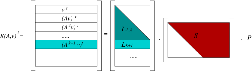
Figure 1: principle of the computation of $P_{A,v}^{min}$

Now the trick is to notice that the vector $m=L_{k+1}L_{1\dots k}^{-1}$ gives the opposites of the coefficients of $P_{A,v}^{min}$. Indeed, let us define $X=K_{A,v}^{t}$

$$X_{1\dots n,k+1}=(A^{k}v)^{t}=\sum_{i=0}^{k-1}{m_{i}(A^{i}v)^{t}}=m\cdot X_{1\dots n,1\dots k}$$

where $P_{A,v}^{min}(X)=X^{k}-m_{k}X^{k-1}-\dots-m_{1}X-m_{0}$.

Thus

$$L_{k+1}SP=m\cdot L_{1\dots k}SP$$

And finally $m=L_{k+1}.L_{1\dots k}^{-1}$

The algorithm is then straightforward:

Algorithm 1 MinPoly : Minimal Polynomial of $A$ and $v$

0:  $A$ a $n\times n$ matrix and $v$ a vector over a field

0:  $P_{\text{min}}^{A,v}(X)$ the minimal polynomial of the sequence of vectors $(A^{i}v)_{i}$

1:  $K_{1\dots n,1}=v$

2:  for $i=1$ to $\text{log}_{2}(n)$ do

3:     $K_{1\dots n,2^{i}\dots 2^{i+1}-1}=A^{2^{i-1}}K_{1\dots n,1\dots 2^{i}-1}$

4:  end for

5:  $(L,S,P)=\mbox{LSP}(K^{t}),k=\mbox{rank}(K)$

6:  $m=L_{k+1}.L_{1\dots k}^{-1}$

7:  return $P_{\text{min}}^{A,v}(X)=X^{k}+\sum_{i=0}^{k-1}{m_{i}X^{i}}$

The dominant operation in this algorithm is the computation of $K$, in $log_{2}n$ matrix multiplications, i.e. in ${\cal O}(n^{\omega}logn)$ algebraic operations. The LSP factorization requires ${\cal O}(n^{\omega})$ operations and the triangular system resolution, ${\cal O}(n^{2})$. The algebraic time complexity of this algorithm is thus ${\cal O}(n^{\omega}logn)$.

When using classical matrix multiplications (assuming $\omega=3$), it is preferable to compute the Krylov matrix $K$ by $k$ successive matrix vector products. The number of field operations is then ${\cal O}(n^{3})$.

It is also possible to merge the creation of the Krylov matrix and its LSP factorization so as to avoid the computation of the last $n-k$ Krylov iterates with an early termination approach. This reduces the time complexity to ${\cal O}(n^{\omega}log(k))$ for fast matrix arithmetic, and ${\cal O}(n^{2}k)$ for classic matrix arithmetic.

Note that choosing $v$ randomly makes the algorithm Monte-Carlo for the computation of the minimal polynomial of A.

2.2 LU-Krylov algorithm

We present here an algorithm, using the previous computation of the minimal polynomial of the sequence $(A^{i}v)_{i}$ to compute the characteristic polynomial of $A$. The previous algorithm produces the $k$ first independent Krylov iterates of $v$. They can be viewed as a basis of an invariant subspace under the action of $A$, and if $P_{A,v}^{min}=P_{A}^{min}$, this subspace is the first invariant subspace of $A$. The idea is to make use of the elimination performed on this basis to compute a basis of its supplementary subspace. Then a recursive call on this second basis will decompose this subspace into a series of invariant subspaces generated by one vector.

The algorithm is the following, where $k$, $P$, and $S$ come from the notation of algorithm 1.

Algorithm 2 LUK : LU-Krylov algorithm

0:  $A$ a $n\times n$ matrix over a field

0:  $P_{\text{char}}^{A}(X)$ the characteristic polynomial of $A$

1:  Pick a random vector $v$

2:  $P_{\text{min}}^{A,v}(X)=MinPoly(A,v)$ of degree $k${$X=\left[\begin{array}[]{c}L_{1}\\ L_{2}\end{array}\right][S_{1}|S_{2}]P$ is computed}

3:  if  $(k=n)$  then

4:     return $P^{A}_{\text{char}}=P^{A,v}_{\text{min}}$

5:  else

6:     $A^{\prime}=PA^{T}P^{T}=\left[\begin{array}[]{cc}A^{\prime}_{11}&A^{\prime}_{12}\\ A^{\prime}_{21}&A^{\prime}_{22}\end{array}\right]$ where $A^{\prime}_{11}$ is $k\times k$.

7:     $P^{A^{\prime}_{22}-A^{\prime}_{21}S_{1}^{-1}S_{2}}_{\text{char}}(X)=LUK(A^{\prime}_{22}-A^{\prime}_{21}S_{1}^{-1}S_{2})$

8:     return $P^{A}_{\text{char}}(X)=P^{A,v}_{\text{min}}(X)\times P^{A^{\prime}_{22}-A^{\prime}_{21}S_{1}^{-1}S_{2}}_{\text{char}}(X)$

9:  end if

Theorem 2.1.

The algorithm LU-Krylov computes the characteristic polynomial of an $n\times n$ matrix $A$ in ${\cal O}(n^{3})$ field operations.

Proof.

Let us use the following notations

$$X=\left[\begin{array}[]{c}L_{1}\\ L_{2}\end{array}\right][S_{1}|S_{2}]P$$

As we already mentioned, the first $k$ rows of $X$ ($X_{1\dots k,1\dots n}$) form a basis of the invariant subspace generated by $v$. Moreover we have

$$X_{1..k}A^{T}=C_{P^{A,v}_{\text{min}}}^{T}X_{1..k}$$

Indeed

$$\forall i<k\ X_{i}A^{T}=\left(A^{i-1}v\right)^{T}A^{T}=\left(A^{i}v\right)^{T}=X_{i+1}$$

and

$$X_{k}A^{T}=\left(A^{k-1}v\right)^{T}A^{T}=\left(A^{k}v\right)^{T}=\sum_{i=0}^{k-1}{m_{i}\left(A^{i}v\right)^{T}}$$

The idea is now to complete this basis into a basis of the whole space. Viewed as a matrix, this basis form the $n\times n$ invertible matrix $\overline{X}$. It is defined as follows:

$$\overline{X}=\underbrace{\left[\begin{array}[]{cc}L_{1}&0\\ 0&I_{n-k}\end{array}\right]}_{\overline{L}}\underbrace{\left[\begin{array}[]{cc}S_{1}&S_{2}\\ 0&I_{n-k}\end{array}\right]}_{\overline{S}}P=\left[\begin{array}[]{c}X_{1\dots k,1\dots n}\\ \left[\begin{array}[]{cc}0&I_{n-k}\end{array}\right]P\end{array}\right]$$

Let us compute

$$\overline{X}A^{T}\overline{X}^{-1} = \left[\begin{array}[]{c|c}\hskip 22.76219ptC^{T}&0\\ \hline\cr\lx@intercol\hfil\left[\begin{array}[]{cc}0&I_{n-k}\end{array}\right]PA^{T}P^{T}{\overline{S}}^{-1}{\overline{L}}^{-1}\hfil\lx@intercol\end{array}\right]$$

$$= \left[\begin{array}[]{c|c}\hskip 17.07164ptC^{T}&0\\ \hline\cr\lx@intercol\hfil\left[\begin{array}[]{cc}A^{\prime}_{21}&A^{\prime}_{22}\end{array}\right]{\overline{S}}^{-1}{\overline{L}}^{-1}\hfil\lx@intercol\end{array}\right]$$

$$= \left[\begin{array}[]{c|c}C^{T}&0\\ \hline\cr Y&X_{2}\end{array}\right]$$

with

$$X_{2}=A^{\prime}_{22}-A^{\prime}_{21}S_{1}^{-1}S_{2}$$

By a similarity transformation, we thus have reduced $A$ to a block triangular matrix. Then the characteristic polynomial of $A$ is the product of the characteristic polynomial of these two diagonal blocks:

$$P_{\text{char}}^{A}=P^{A,v}_{\text{min}}\times P^{A^{\prime}_{22}-A^{\prime}_{21}S_{1}^{-1}S_{2}}_{\text{char}}$$

Now for the time complexity, we will denote by $T_{\tt LUK}(n)$ the number of field operations for this algorithm applied on a $n\times n$ matrix, by $T_{\tt minpoly}(n,k)$ the cost of the algorithm 1 applied on a $n\times n$ matrix having a degree $k$ minimal polynomial, by $T_{\tt LSP}(m,n)$ the cost of the LSP factorization of a $m\times n$ matrix, by $T_{\tt trsm}(m,n)$ the cost of the simultaneous resolution of $m$ triangular systems of dimension $n$, and by $T_{\tt MM}(m,k,n)$ the cost of the multiplication of a $m\times k$ matrix by a $k\times n$ matrix.

The values of $T_{\tt LSP}$ and $T_{\tt trsm}$ can be found in [6]. Then, using classical matrix arithmetic, we have:

$$T_{\tt LUK}(n) = T_{\tt minpoly}(n,k)+T_{\tt LSP}(k,n)+T_{\tt trsm}(n-k,k)$$

$$+T_{\tt mm}(n-k,k,n-k)+T_{\tt LUK}(n-l)$$

$$= {\cal O}(n^{2}k+k^{2}n+k^{2}(n-k)+k(n-k)^{2})$$

$$+T_{\tt LUK}(n-k)$$

$$= {\cal O}(\sum_{i}{n^{2}k_{i}+k_{i}^{2}n})$$

$$= {\cal O}(n^{3})$$

The latter being true since $\sum_{i}k_{i}=n$ and $\sum_{i}{k_{i}^{2}}\leq n^{2}$.

∎

Note that when using fast matrix arithmetic, it is no longer possible to sum the $log(k_{i})$ into $log(n)$ or the $k_{i}^{\omega-2}n^{2}$ into $n^{\omega}$, so this prevents us from getting the best known time complexity of $n^{\omega}log(n)$ with this algorithm. We will now focus on the second algorithm of Keller-Gehrig achieving this best known time complexity.

2.3 Improving Keller-Gehrig’s branching algorithm

In [18], Keller-Gehrig presents a so called branching algorithm, computing the characteristic polynomial of a $n\times n$ matrix over a field $K$ in the best known time complexity of $n^{\omega}log(n)$ field operations.

The idea is to compute the Krylov iterates of a several vectors at the same time. More precisely, the algorithm computes a sequence of $n\times n$ matrices $(V_{i})_{i}$ whose columns are the Krylov’s iterates of vectors of the canonical basis. $U_{0}$ is the identity matrix (every vector of the canonical basis is present). At the $i$-th iteration, the algorithm computes the following $2^{i}$ Krylov’s iterates of the remaining vectors. Then a Gaussian elimination determines the linear dependencies between them so as to form $V_{i+1}$ by picking the $n$ linearly independent vectors. The algorithm ends when each $V_{i}$ is invariant under the action of $A$. Then the matrix $V^{-1}AV$ is block diagonal with companion blocks on the diagonal. The polynomials of these blocks are the minimal polynomials of the sequence of Krylov’s iterates, and the characteristic polynomial is the product of the polynomials associated to these companion blocks.

The linear dependencies removal is performed by a step-form elimination algorithm defined by Keller-Gehrig. Its formulation is rather sophisticated, and we propose to replace it by the column reduced form algorithm (algorithm 3) using the more standard LQUP

Algorithm 3 ColReducedForm

0:  $A$ a $m\times n$ matrix of rank $r$ ($m,n\geq r$) over a field

0:  $A^{\prime}$ a $m\times r$ matrix formed by r linearly independent columns of $A$

1:  $(L,Q,U,P,r)=\text{LQUP}(A^{T})$ ($r=rank(A)$)

2:  return $([I_{r}0](Q^{T}A^{T}))^{T}$

factorization (described in [14]). More precisely, the step form elimination of Keller-Gehrig, the LQUP factorization of Ibarra & Al. and the echelon elimination (see e.g. [23]) are equivalent and can be used to determine the linear dependencies in a set of vectors.

Algorithm 4 KGB: Keller-Gehrig Branching algorithm

0:  $A$ a $n\times n$ matrix over a field

0:  $P_{\text{char}}^{A}(X)$ the characteristic polynomial of $A$

1:  $i=0$

2:  $V_{0}=I_{n}=(V_{0,1},V_{0,2},\dots,V_{0,n})$

3:  $B=A$

4:  while ($\exists k,V_{k}$ has $2^{i}$ columns) do

5:     for all j do

6:        if  ( $V_{i,j}$ has strictly less than $2^{i}$ columns ) then

7:           $W_{j}=V_{i,j}$

8:        else

9:           $W_{j}=\left[V_{i,j}|BV_{i,j}\right]$

10:        end if

11:     end for

12:     $W=(W_{j})_{j}$

13:     $V_{i+1}=\text{ColReducedForm}(W)${$V_{i+1,j}$ are the remaining vectors of $W_{j}$ in $V_{i+1}$}

14:     $B=B\times B$

15:     $i=i+1$

16:  end while

17:  for all $j$ do

18:     compute $P_{j}$ the minimal polynomial of the sequence of vectors of $V_{i-1,j}$, using algorithm 1

19:  end for

20:  return $\Pi_{j}{P_{j}}$

Our second improvement is to apply the idea of algorithm 1 to compute polynomials associated to each companion block, instead of computing $V^{-1}AV$. The Krylov’s iterates are already computed, and the last call to ColReducedForm performed the elimination on it, so there only remains to solve the triangular systems so as to get the coefficients of each polynomial.

Algorithm 4 sums up these modifications. The operations in the while loop have a ${\cal O}(n^{\omega})$ algebraic time complexity. This loop is executed at most $\text{log}(n)$ times and the algebraic time complexity of the algorithm is therefore ${\cal O}(n^{\omega}\text{log}(n))$. More precisely it is ${\cal O}(n^{\omega}\text{log}(k_{\text{max}}))$ where $k_{\text{max}}$ is the degree of the largest invariant factor.

2.4 Experimental comparisons

To implement these two algorithms, we used a finite field representation over double size floating points: modular<double> (see [6]) and the efficient routines for finite field linear algebra FFLAS-FFPACK presented in [6, 5]. The following experiments used a classic matrix arithmetic. We ran them on a series of matrices of order $300$ which Frobenius normal forms had different number of diagonal companion blocks. Figure 2 shows the computational time on a Pentium IV 2.4Ghz with 512Mb of RAM.

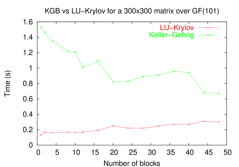
Figure 2: LU-Krylov vs. KGB

It appears that LU-Krylov is faster than KGB on every matrices. This is due to the extra $\text{log}(n)$ factor in the time complexity of the latter. One can note that the computational time of KGB is decreasing with the number of blocks. This is due to the fact that the $\text{log}(n)$ is in fact $\text{log}(k_{\text{max}}$ where $k_{\text{max}}$ is the size of the largest block. This factor is decreasing when the number of blocks increases. Conversely, LU-Krylov computational time is almost constant. It slightly increases, due to the increasing number of rectangular matrix operations. The latter being less efficient than square matrix operations.

3 Toward an optimal algorithm

As mentioned in the introduction, the best known algebraic time complexity for the computation of the characteristic polynomial is not optimal in the sense that it is not ${\cal O}(n^{\omega})$ but ${\cal O}(n^{\omega}\text{log}(n))$. However, Keller-Gehrig gives a third algorithm (let us name it KG3), having this time complexity but only working on generic matrices.

To get rid of the extra $\text{log}(n)$ factor, it is no longer based on a Krylov approach. The algorithm is inspired by a ${\cal O}(n^{3})$ algorithm by Danilevski (described in [13]), improved into a block algorithm. The genericity assumption ensures the existence of a series of similarity transformations changing the input matrix into a companion matrix.

3.1 Comparing the constants

The optimal “big-O” complexity often hides a large constant in the exact expression of the time complexity. This makes these algorithms impracticable since the improvement induced is only significant for huge matrices. However, we show in the following lemma that the constant of KG3 has the same magnitude as the one of LUK.

Lemma 3.1.

The computation of the characteristic polynomial of a $n\times n$ generic matrix using KG3 algorithm requires $K_{\omega}n^{\omega}+o(n^{\omega})$ algebraic operations, where

$$K_{\omega} = C_{\omega}\left[-\frac{2^{\omega-2}}{2(2^{\omega-2}-1)(2^{\omega-1}-1)(2^{\omega}-1)}-\frac{1}{2^{\omega}-1}\right.$$

$$+\frac{1}{(2^{\omega-2}-1)(2^{\omega-1}-1)}-\frac{3}{2^{\omega-1}-1}+\frac{2}{2^{\omega-2}-1}$$

$$\left.+\frac{1}{(2^{\omega-2}-1)(2^{\omega}-1)}+\frac{2^{\omega-2}}{2(2^{\omega-2}-1)(2^{\omega-1}-1)^{2}}\right]$$

and $C_{\omega}$ is the constant in the algebraic time complexity of the matrix multiplication.

The proof and a description of the algorithm are given in appendix A.

In particular, when using classical matrix arithmetic ($\omega=3,C_{\omega}=2$), we have on the one hand $K_{\omega}=176/63\approx 2.794$.

On the other hand, the algorithm 2 called on a generic matrix simply computes the $n$ Krylov vectors $A^{i}v$ ($2n^{3}$ operations), computes the LUP factorization of these vectors ($2/3n^{3}$ operations) and the coefficients of the polynomial by the resolution of a triangular system (${\cal O}(n^{2})$). Therefore, the constant for this algorithm is $2+2/3\approx 2.667$. These two algorithms have thus a similar algebraic complexity, LU-Krylov being slightly faster than Keller-Gehrig’s third algorithm. We now compare them in practice.

3.2 Experimental comparison

We claim that the study of precise algebraic time complexity of these algorithms is worth-full in practice. Indeed these estimates directly correspond to the computational time of these algorithms applied over finite fields. Therefore we ran these algorithms on a small prime finite field (word size elements with modular arithmetic). Again we used modular<double> and FFLAS-FFPACK. These routines can use fast matrix arithmetic, we, however, only used classical matrix multiplication so as to compare two ${\cal O}(n^{3})$ algorithms having similar constants ($2.67$ for LUK and $2.794$ for KG3). We used random dense matrices over the finite field $\mathbb{Z}_{65521}$, as generic matrices. We report the computational speed in Mfops (Millions of field operations per second) for the two algorithms on figure 3:

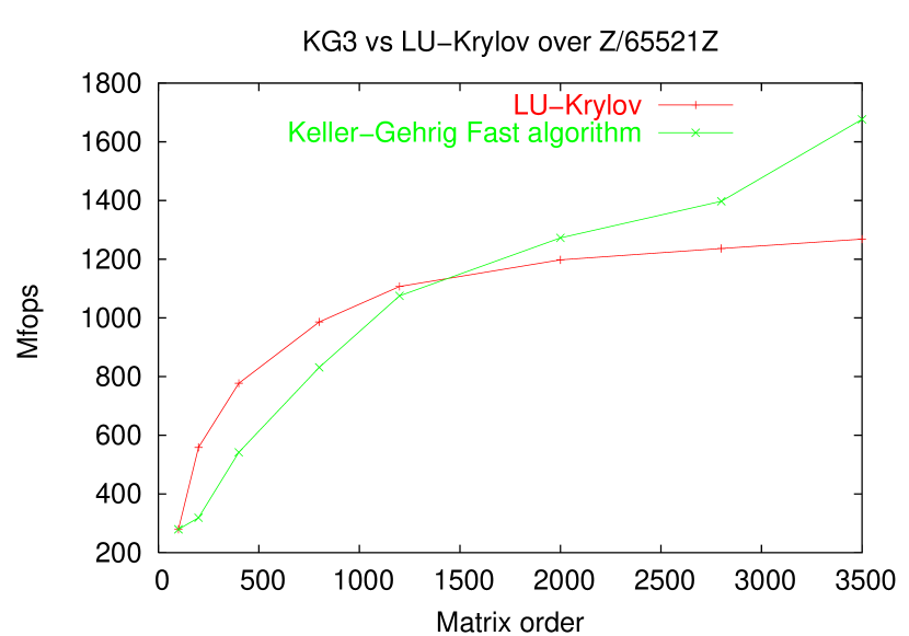
Figure 3: LUK vs. KG3: speed comparison

It appears that LU-Krylov is faster than KG3 for small matrices, but for matrices of order larger than 1500, KG3 is faster. Indeed, the ${\cal O}(n^{3})$ operations are differently performed: LU-Krylov computes the Krylov basis by $n$ matrix-vector products, whereas KG3 only uses matrix multiplications. Now, as the order of the matrices gets larger, the BLAS routines provides better efficiency for matrix multiplications than for matrix vector products. Once again, algorithms exclusively based on matrix multiplications are preferable: from the complexity point of view, they make it possible to achieve ${\cal O}(n^{\omega})$ time complexity. In practice, they promise the best efficiency thanks to the BLAS better memory management.

4 Over the Integers

There exist several algorithms to compute the characteristic polynomial of an integer matrix. A first idea is to perform the algebraic operations over the ring of integers, using exact divisions [1] or by avoiding divisions [3, 15, 8, 17]. We focus here on field approaches. Concerning the bit complexity of this computation, a first approach, using Chinese remaindering gives ${\cal O}\text{\~{\ }}(n^{\omega+1}\text{log}\|A\|)$ bit operations (${\cal O}\text{\~{\ }}$ is the “soft-O” notation, hiding logarithmic and poly-logarithmic factors in $n$ and $\|A\|$). Baby-step Giant-step techniques applied by Eberly [8] improves this complexity to ${\cal O}\text{\~{\ }}(n^{3.5}\text{log}\|A\|)$ (using classic matrix arithmetic). Lastly, the recent improvement of [17, §7.2], combining Coppersmith’s block-Wiedemann techniques [4, 16, 26, 25] set the best known exponent for this computation to $2.697263$ using fast matrix arithmetic.

Our goal here is not to give an exhaustive comparison of these methods, but to show that a straightforward application of our finite field algorithm LU-Krylov is already very efficient and can outperform the best existing softwares.

A first deterministic algorithm, using Chinese remaindering is given in section 4.1. Then we improve it in section 4.2 into a probabilistic algorithm by using the early termination technique of [7, §3.3]. Therefore, the minimal number of homomorphic computations is achieved. Now, for the sparse case, a recent alternative [24], also developed in [17, §7.2], change the Chinese remaindering by a Hensel p-adic lifting in order to improve the binary complexity of the algorithm. In section 4.4, we combine some of these ideas with the Sparse Integer Minimal Polynomial computation of [7] and our dense modular characteristic polynomial to present an efficient practical implementation.

4.1 Dense deterministic : Chinese remaindering

The first naive way of computing the characteristic polynomial is to use Hadamard’s bound [10, Theorem 16.6] to show that any integer coefficient of the characteristic polynomial has the order of $n$ bits:

Lemma 4.1.

Let $A\in\mathbb{Z}^{n\times n}$, with $n\geq 4$, whose coefficients are bounded in absolute value by $B>1$. The coefficients of the characteristic polynomial of $A$ have less than $\lceil\frac{n}{2}\left(\log_{2}(n)+\log_{2}(B^{2})+1.6669\right)\rceil$ bits.

Proof.

$c_{i}$, the $i$-th coefficient of the characteristic polynomial, is a sum of all the $(n-i)\times(n-i)$ diagonal minors of $A$. It is therefore bounded by ${n\choose i}\sqrt{(n-i)B^{2}}^{(n-i)}$. The lemma is true for $i=n$ since the characteristic polynomial is unitary and also true for $i=0$ by Hadamard’s bound. Now, using Stirling’s formula ($n!<(1+\epsilon)\sqrt{2\pi n}\frac{n^{n}}{e^{n}}$), one gets ${n\choose i}<\frac{1+\epsilon}{\sqrt{2\pi}}\sqrt{\frac{n}{i(n-i)}}\left(\frac{n}{i}\right)^{i}\left(\frac{n}{n-i}\right)^{n-i}$. Thus $\log_{2}(c_{i})<\frac{n}{2}\left(\log_{2}(n)+\log_{2}(B^{2})+C\right)-H$. Well, suppose on the first hand that $i\leq\frac{n}{2}$, then $H\sim(\frac{1}{ln(2)}-1+C)\frac{n}{2}+\frac{3i^{2}}{nln(2)}+\frac{C-3}{2}i-\frac{5i}{2ln(2)}$. On the second hand, if $(n-i)\leq\frac{n}{2}$, then $H\sim(\frac{1}{ln(2)}-1)n+\frac{3k^{2}}{nln(2)}+\frac{C+5}{2}k-\frac{7k}{2ln(2)}$, where $k=n-i$. Both equivalences are positive as soon as $C<1.6668979201$. ∎

For example, the characteristic polynomial of

$$\left[\begin{array}[]{ccccc}1&1&1&1&1\\ 1&1&-1&-1&-1\\ 1&-1&1&-1&-1\\ 1&-1&-1&1&-1\\ 1&-1&-1&-1&1\end{array}\right]$$

is $X^{5}-5X^{4}+40X^{2}-80X+48$ and $80={5\choose 1}\sqrt{4}^{4}$ is greater than Hadamard’s bound $56$, but less than our bound $1004.4$.

Note that this bound improves the one used in [11, lemma 2.1] since $1.6669<2+\text{log}_{2}(e)\approx 3.4427$.

Now, using fast integer arithmetic and the fast Chinese remaindering algorithm [10, Theorem 10.25], one gets the overall complexity for the dense integer characteristic polynomial via Chinese remaindering of

$$O(n^{4}(log(n)+log(B))).$$

Well, as we see in next section, to go faster, the idea is actually to stop the remaindering earlier. Indeed, the actual coefficients can be much smaller than the bound of lemma 4.1.

4.2 Dense probabilistic Monte-Carlo : early termination

We just use the early termination of [7, §3.3]. There it is used to stop the remaindering of the integer minimal polynomial, here we use it to stop the remaindering of the characteristic polynomial:

Lemma 4.2.

[7] Let $v\in\mathbb{Z}$ be a coefficient of the characteristic polynomial, and $U$ be a given upper bound on $|v|$. Let $P$ be a set of primes and let $\{p_{1}\ldots p_{k},p^{*}\}$ be a random subset of $P$. Let $l$ be a lower bound such that $p^{*}>l$ and let $M=\prod_{i=1}^{k}p_{i}$. Let $v_{k}=v\mod M$, $v^{*}=v\mod p^{*}$ and $v_{k}^{*}=v_{k}\mod p^{*}$ as above. Suppose now that $v_{k}^{*}=v^{*}$. Then $v=v_{k}$ with probability at least $1-\frac{\log_{l}(\frac{U-v_{k}}{M})}{|P|}$.

The proof is that of [7, lemma 3.1]. The probabilistic algorithm is then straightforward: after each modular computation of a characteristic polynomial, the algorithm stops if every coefficient is unchanged. It is of the Monte-Carlo type: always fast with a controlled probability of success. The probability of success is bounded by the probability of lemma 4.2. In practice this probability is much higher, since the $n$ coefficients are checked. But since they are not independent, we are not able to produce a tighter bound.

4.3 Experimental results

We implemented these two methods using LU-Krylov over finite fields as described in section 2.4. The choice of moduli is there linked to the constraints of the matrix multiplication of FFLAS. Indeed, the wrapping of numerical BLAS matrix multiplication is only valid if $n(p-1)^{2}<2^{53}$ (the result can be stored in the $53$ bits of the double mantissa). Therefore, we chose to sample the primes between $2^{m}$ and $2^{m+1}$ (where $m=\lfloor 25.5-\frac{1}{2}\text{log}_{2}(n)\rfloor$). This set was always sufficient in practice. Even with $5000\times 5000$ matrices, $m=19$ and there are $38658$ primes between $2^{19}$ and $2^{20}$. Now if the coefficients of the matrix are between $-1000$ and $1000$, the upper bound on the coefficients of the characteristic polynomial is $\text{log}_{2^{m}}(U)\approx 4458.7$. Therefore, the probability of finding a bad prime is lower than $4458.7/38658\approx 0.1153$. Then performing a couple a additional modular computations to check the result will improve this probability. In this example, only 17 more computations (compared to the $4459$ required for the deterministic computation) are enough to ensure a probability of error lower than $2^{-50}$, for which Knuth [19, §4.5.4] considers that there is more chances that cosmic radiations perturbed the output!

In the following, we denote by ILUK-det the deterministic algorithm of section 4.1, by ILUK-prob the probabilistic algorithm of section 4.2 with primes chosen as above and by ILUK-QD the quasi-deterministic algorithm obtained by applying ILUK-prob plus a sufficient number of modular computations to ensure a probability of failure lower than $2^{-50}$.

$n$	Maple	Magma	ILUK-det	ILUK-prob	ILUK-QD
100	163s	0.34s	0.22s	0.17s	0.2s
200	3355s	4.45s	4.42s	3.17s	3.45s
		11.1Mb	3.5Mb	3.5Mb	3.5Mb
400	74970s	69.8s	91.87s	64.3s	66.75s
		56Mb	10.1Mb	10.1Mb	10.1Mb
800		1546s	1458s	1053s	1062s
		403Mb	36.3Mb	36.3Mb	36.3Mb
1200		8851s	7576s	5454s	5548s
		1368Mb	81Mb	81Mb	81Mb
1500		MT	21082s	15277s	15436s
			136Mb	136Mb	136Mb
2000		MT	66847s	46928s
			227Mb	227Mb
2500		MT	169355s	124505s
			371Mb	371Mb
3000		MT	349494s	254358s
			521Mb	521Mb

Table 1: Characteristic polynomial of a dense integer matrix of order $n$ (computation time in seconds and memory allocation in Mb)

We report in table 1 the timings of their implementations, compared to the timings of the same computation using Maple-v9 and Magma-2.11. We ran these tests on an athlon 2200 (1.8 Ghz) with 2Gb of RAM, running Linux-2.4. The matrices are formed by integers chosen uniformly between 0 and 10: therefore, their minimal polynomial equals their characteristic polynomial.

The implementation of Berkowitz algorithm used by Maple has prohibitive computational timings. Magma is much faster thanks to a $p\_$adic algorithm (probabilistic ?) . However, no literature exists to our knowledge, describing this algorithm. Our deterministic algorithm has similar computational timings and gets faster for large matrices. For matrices of order over $800$, magma tries to allocate more than 2Gb of RAM, and the computation crashes (denoted by MT as Memory Thrashing). The memory usage of our implementations is much smaller than in magma, and makes it possible to handle larger matrices.

The probabilistic algorithm ILUK-prob improves the computational time of the deterministic one of roughly $27$ %, and the cost of the extra checks done by ILUK-QD is negligible.

However, this approach does not take advantage of the structure of the matrix nor of the degree of the minimal polynomial, as magma seems to do. In the following, we will describe a third approach to fill this gap.

4.4 Structured or Sparse probabilistic Monte-Carlo

By structured or sparse matrices we mean matrices for which the matrix-vector product can be performed with less than $n^{2}$ arithmetic operations or matrices having a small minimal polynomial degree. In those cases our idea is to compute first the integer minimal polynomial via the specialized methods of [7, §3] (denoted by IMP), to factor it and them to simply recover the factor exponents by a modular computation of the characteristic polynomial. The overall complexity is not better than e.g. [24, 17] but the practical speeds shown on table 2 speak for themselves. The algorithm is as follows:

Algorithm 1 CIA : Characteristic polynomial over Integers Algorithm

0:  $A\in\mathbb{Z}^{n\times n}$, even as a blackbox, $\epsilon$.

0:  The characteristic polynomial of $A$ with a probability of $1-\epsilon$.

1:  $\eta=1-\sqrt{1-\epsilon}$

2:  $P_{\text{min}}^{A}$ = IMP($A,\eta$) via [7, §3].

3:  Factor $P_{\text{min}}^{A}$ over the integers, e.g. by Hensel’s lifting.

4:  $B=2^{\frac{n}{2}\left(\log_{2}(n)+\log_{2}(||A||^{2})+1.6669\right)}$

5:  Choose a random prime $p$ in a set of $\frac{1}{\eta}\text{log}_{2}(\sqrt{n+1}\ 2^{n+1}B+1)$ primes.

6:  Compute $P_{p}$ the characteristic polynomial of $A$ mod $p$ via LUK.

7:  for all $f_{i}$ irreducible factor of $P_{\text{min}}^{A}$ do

8:     Compute $\overline{f}_{i}\equiv f_{i}\mod p$.

9:     Find $\alpha_{i}$ the multiplicity of $\overline{f}_{i}$ within $P_{p}$.

10:     if $\alpha_{i}$ == 0 then

11:        Return “FAIL”.

12:     end if

13:  end for

14:  Compute $P_{\text{char}}^{A}=\prod f_{i}^{\alpha_{i}}=X^{n}-\sum_{i=0}^{n-1}{a_{i}X^{i}}$.

15:  if  ($\sum\alpha_{i}\text{degree}(f_{i})\neq n$)  then

16:     Return “FAIL”.

17:  end if

18:  if  ($Trace(A)\neq a_{n-1}$ ) then

19:     Return “FAIL”.

20:  end if

21:  Return $P_{\text{char}}^{A}$.

Theorem 4.3.

Algorithm 1 is correct. It is probabilistic of the Monte-Carlo type. Moreover, most cases where the result is wrong are identified.

Proof.

Let $P^{\text{min}}$ be the integer minimal polynomial of $A$ and $\tilde{P}^{\text{min}}$ the result of the call to IMP.

With a probability of $\sqrt{1-\epsilon}$, $P^{\text{min}}=\tilde{P}^{\text{min}}$. Then the only problem that can occur is that an irreducible factor of $P^{\text{min}}$ divides another factor when taken modulo $p$, or equivalently, that $p$ divides the resultant of these polynomials. Now from [10, Algorithm 6.38] and lemma 4.1 an upper bound on the size of this resultant is $\text{log}_{2}(\sqrt{n+1}\ 2^{n+1}B+1)$. Therefore, the probability of choosing a bad prime is less than $\eta$. Thus the result will be correct with a probability greater than $1-\epsilon$ ∎

This algorithm is also able to detect most erroneous results and return “FAIL” instead. We call it therefore “Quasi-Las-Vegas”.

The first case is when $P^{\text{min}}=\tilde{P}^{\text{min}}$ and a factor of $P^{\text{min}}$ divides another factor modulo $p$. In such a case, the exponent of this factor will appear twice in the reconstructed characteristic polynomial. The overall degree being greater than $n$, FAIL will be returned.

Now, if $P^{\text{min}}\neq\tilde{P}^{\text{min}}$, the tests $\alpha_{i}>0$ will detect it unless $\tilde{P}^{\text{min}}$ is a divisor of $P^{\text{min}}$, say $P^{\text{min}}=\tilde{P}^{\text{min}}Q$. In that case, on the one hand, if $Q$ does not divide $\tilde{P}^{\text{min}}$ modulo $p$, the total degree will be lower than $n$ and FAIL will be returned. On the other hand, a wrong characteristic polynomial will be reconstructed, but the trace test will detect most of these cases.

We now compare our algorithms to magma. In table 2, we denote by $d$ the degree of the integer minimal polynomial and by $\omega$ the average number of nonzero elements per row within the sparse matrix. CIA is written in C++ and uses different external modules: the integer minimal polynomial is computed with LinBox via [7, §3], the polynomial factorization is computed with NTL via Hensel’s factorization.

Matrix	$A$	$U^{-1}AU$	$A^{T}A$	B	$U^{-1}BU$	$B^{T}B$
$n$	300	300	300	600	600	600
$d$	75	75	21	424	424	8
$\omega$	1.9	300	2.95	4	600	13
ILUK-prob	1.3	1.5	18.3	31.8	34.9	120.0
ILUK-det	37.5	121.7	265.0	310	3412	422.3
Magma	1.4	16.5	0.2	6.2	184.0	6.0
CIA	0.32	3.72	0.86	4.51	325.1	2.4
IMP	0.01	3.38	0.01	1.49	322.1	0.04
Fact	0.05	0.05	0.01	0.76	0.76	0.01
LUK+Mul	0.26	0.29	0.84	2.26	2.26	2.30

Table 2: CIA on sparse or structured matrices

We show the computational times of algorithm 1 (CIA), decomposed into the time for the integer minimal polynomial computation (IMP), the factorization of this polynomial (Fact), the computation of the characteristic polynomial and the computation of the multiplicities (LUK+Mul). They are compared to the timings of the algorithms of section 4.1 and 4.2.

We used two sparse matrices $A$ and $B$ of order $300$ and $600$, having a minimal polynomial of degree respectively $75$ and $424$. $A$ is the almost empty matrix Frob08blocks and is in Frobenius normal form with $8$ companion blocks and $B$ is the matrix ch5-5.b3.600x600.sms presented in [7].

On these matrices magma is pretty efficient thanks to their sparsity. The early termination in ILUK-prob gives similar timings for $A$, since the coefficients of its characteristic polynomial are small. But this is not the case with $B$. ILUK-det performs many useless operations since the Hadamard bound is well overestimating the size of the coefficients. CIA also takes advantage of both the sparsity and the low degree of the minimal polynomial. It is actually much faster than magma for $A$ and is slightly faster for $B$ (the degree of the minimal polynomial is bigger).

Then, we made these matrices dense with an integral similarity transformation. The lack of sparsity slows down both magma and CIA, whereas ILUK-prob maintains similar timings. ILUK-det is much slower because the bigger size of the matrix entries increases the Hadamard bound.

Lastly, we used symmetric matrices with small minimal polynomial ($A^{T}A$ and $B^{T}B$). The bigger size of the coefficients of the characteristic polynomial makes the Chinese remainder methods of ILUK-prob and ILUK-det slower. CIA is still pretty efficient ( the best on $B^{T}B$ ), but magma appears to be extremely fast on $A^{T}A$.

We report in table 3 on some comparisons using other sparse matrices.

Matrix	$n$	$\omega$	magma	CIA	ILUK-QD
TF12	552	7.6	10.03s	6.93s	51.84s
Tref500	500	16.9	108.1s	64.58s	335.04s
mk9b3	1260	3	77.02s	35.74s	348.31s

Table 3: CIA on other sparse matrices

To conclude, ILUK-det is always too expensive, although it has better timings than magma for large dense matrices (cf. table 1). ILUK-prob is well suited for every kind of matrix having a characteristic polynomials with small coefficients. Now with sparse or structured matrices, magma and CIA are more efficient; CIA being almost always faster.

5 Conclusion

We presented a new algorithm for the computation of the characteristic polynomial over a finite field, and proved its efficiency in practice. We also considered Keller-Gehrig’s third algorithm and showed that its generalization would be not only interesting in theory but produce a practicable algorithm.

We applied our algorithm for the computation of the integer characteristic polynomial in two ways: a combination of Chinese remaindering and early termination for dense matrix computations, and a mixed blackbox-dense algorithm for sparse or structured matrices. These two algorithm outperform the existing software for this task. Moreover we showed that the recent improvements of [24, 17] should be highly practicable since the successful CIA algorithm is inspired by their ideas. It remains to show how much they improve the simple approach of CIA.

To improve the dense matrix computation over a finite field, one should consider the generalization of Keller-Gehrig’s third algorithm. At least some heuristics could be built: using row-reduced form elimination to give produce generic rank profile.

Lastly, concerning the sparse computations, the blackbox algorithms of [27] and of [9], could handle huge sparse matrices (no dense computation is used as in CIA). But one should study how their use of preconditionners, expensive in practice, penalize them.

Appendix A On Keller-Gehrig’s third algorithm

We first recall the principle of this algorithm, so as to determine the exact constant in its algebraic time complexity. This advocates for its practicability.

A.1 Principle of the algorithm

First, let us define a $m$-Frobenius form as a $n\times n$ matrix of the shape: $\left[\begin{matrix}0&M_{1}\\ Id_{n-m}&M_{2}\end{matrix}\right]$.

Note that a $1$-Frobenius form is a companion matrix, which characteristic polynomial is given by the opposites of the coefficients of its last column.

The aim of the algorithm is to compute the $1$-Frobenius form $A_{0}$ of $A$ by computing the sequence of matrices $A_{r}=A,\ldots,A_{0},$ where $A_{i}$ has the $2^{i}$-Froebenius form and $r=\left\lceil\log n\right\rceil$. The idea is to compute $A_{i}$ from $A_{i+1}$ by slicing the block $M$ of $A_{i+1}$ into two $n\times 2^{i}$ columns blocks $B$ and $C$. Then, similarity transformations with the matrix

$$U=\left[\begin{matrix}0&C_{1}\\ Id_{n-2^{i}}&C_{2}\end{matrix}\right]$$

will “shift” the block $B$ to the left and generate an identity block of size $2^{i}$ between $B$ and $C$.

Figure 4: Principle of Keller-Gehrig’s third algorithm

More precisely, the algorithm computes the sequence of matrices $A_{i,0}=A_{i+1},A_{i,1},\ldots,A_{i,s_{i}}=A_{i}$, where $s_{i}=\left\lceil n/2^{i}\right\rceil-1$, by the relation $A_{i,j+1}=U_{i,j}^{-1}A_{i,j}U_{i,j}$, whith the notations of figure 4.

As long as $C_{1}$ is invertible, the process will carry on, and make at last the block $B$ disapear from the matrix. This last condition is restricting and is the reason why this algortihm is only valid for generic matrices.

A.2 Proof of lemma 3.1

Lemma 3.1. The computation of the characteristic polynomial of a $n\times n$ generic matrix using the fast algorithm requires $K_{\omega}n^{\omega}+o(n^{\omega})$ algebraic operations, where

$$K_{\omega} = C_{\omega}\left[-\frac{2^{\omega-2}}{2(2^{\omega-2}-1)(2^{\omega-1}-1)(2^{\omega}-1)}-\frac{1}{2^{\omega}-1}\right.$$

$$+\frac{1}{(2^{\omega-2}-1)(2^{\omega-1}-1)}-\frac{3}{2^{\omega-1}-1}+\frac{2}{2^{\omega-2}-1}$$

$$\left.+\frac{1}{(2^{\omega-2}-1)(2^{\omega}-1)}+\frac{2^{\omega-2}}{2(2^{\omega-2}-1)(2^{\omega-1}-1)^{2}}\right]$$

and $C_{\omega}$ is the constant in the algebraic time complexity of the matrix multiplication.

Proof.

We will denote by $X_{a\dots b}$ the submatrix composed by the rows from $a$ to $b$ of the block $X$. For a given $i$, KG3 performs $n/2^{i}$ similarity transformations. Each one of them can be described by the following operations:

1:  $B^{\prime}_{n-2^{i}+1\dots n}=C^{-1}_{1\dots 2^{i}}B_{1\dots 2^{i}}$

2:  $B^{\prime}_{1\dots n-2^{i}}=-C_{2^{i}+1\dots n}B^{\prime}_{n-2^{i}+1\dots n}+B_{2^{i}+1\dots n}$

3:  $C^{\prime}=B^{\prime}C_{\lambda+1\dots\lambda+2^{i}}$

4:  $C^{\prime}_{2^{i}+1\dots 2^{i}+\lambda}+=C_{1\dots\lambda}$

5:  $C^{\prime}_{2^{i}+\lambda+1\dots n}+=C_{2^{i}+\lambda+1\dots n}$

The first operation is a system resolution, and consists in a LUP factorization and two triangular system solve with matrix right hand side. The two following ones are matrix multiplications, and we do not consider the two last ones, since their cost is dominated by the previous ones. The cost of a similarity transformation is then:

$$T_{i,j} = T_{\text{LUP}}(2^{i},2^{i})+2T_{\text{TRSM}}(2^{i},2^{i})$$

$$+T_{\text{MM}}(n-2^{i},2^{i},2^{i})+T_{\text{MM}}(n,2^{i},2^{i})$$

From [6, Lemma 4.1] and [21], we have

$$T_{\text{LUP}}(m,n)=\frac{C_{\omega}}{2^{\omega-1}-2}m^{\omega-1}\left(n-m\frac{2^{\omega-2}-1}{2^{\omega-1}-1}\right)$$

and

$$T_{\text{TRSM}}(2^{i},2^{i})=\frac{C_{\omega}mn^{\omega-1}}{2\left(2^{\omega-1}-1\right)}$$

Therefore

$$T_{i,j} = \frac{C_{\omega}2^{\omega-2}}{2\left(2^{\omega-2}-1\right)\left(2^{\omega-1}-1\right)}(2^{i})^{\omega}+\frac{C_{\omega}}{\left(2^{\omega-2}-1\right)}(2^{i})^{\omega}$$

$$+C_{\omega}(n-2^{i})(2^{i})^{\omega-1}+C_{\omega}n(2^{i})^{\omega-1}$$

$$= C_{\omega}(2^{i})^{\omega}\underbrace{\left(\frac{2^{\omega-3}+2^{\omega-1}-1}{\left(2^{\omega-2}-1\right)\left(2^{\omega-1}-1\right)}-1\right)}_{D_{\omega}}$$

$$+2nC_{\omega}(2^{i})^{\omega-1}$$

And so the total cost of the algorithm is

$$T = \sum_{i=1}^{log(n/2)}{\sum_{j=1}^{n/2^{i}-1}{T_{i,j}}}$$

$$= \sum_{i=1}^{log(n/2)}{\left(\frac{n}{2^{i}}-1\right)C_{\omega}D_{\omega}(2^{i})^{\omega}+2nC_{\omega}(2^{i})^{\omega-1}}$$

$$= C_{\omega}\sum_{i=1}^{log(n/2)}(D_{\omega}-3)n(2^{i})^{\omega-1}+2n^{2}(2^{i})^{\omega-2}$$

$$-D_{\omega}(2^{i})^{\omega}$$

And since

$$\sum_{i=1}^{log(n/2)}{(2^{i})^{x}}=\frac{n^{x}-1}{2^{x}-1}=\frac{n^{x}}{2^{x}-1}+o(n^{x})$$

we get the result:

$$T = n^{\omega}C_{\omega}\left[-\frac{2^{\omega-2}}{2(2^{\omega-2}-1)(2^{\omega-1}-1)(2^{\omega}-1)}-\frac{1}{2^{\omega}-1}\right.$$

$$+\frac{1}{(2^{\omega-2}-1)(2^{\omega-1}-1)}-\frac{3}{2^{\omega-1}-1}+\frac{2}{2^{\omega-2}-1}$$

$$\left.+\frac{1}{(2^{\omega-2}-1)(2^{\omega}-1)}+\frac{2^{\omega-2}}{2(2^{\omega-2}-1)(2^{\omega-1}-1)^{2}}\right]$$

∎

References

- [1] J. Abdeljaoued and G. I. Malaschonok. Efficient algorithms for computing the characteristic polynomial in a domain. Journal of Pure and Applied Algebra, 156:127–145, 2001.
- [2] W. Baur and V. Strassen. The complexity of partial derivatives. Theoretical Computer Science, 22(3):317–330, 1983.
- [3] S. J. Berkowitz. On computing the determinant in small parallel time using a small number of processors. Inf. Process. Lett., 18(3):147–150, 1984.
- [4] D. Coppersmith. Solving homogeneous linear equations over GF[2] via block Wiedemann algorithm. Mathematics of Computation, 62(205):333–350, Jan. 1994.
- [5] J.-G. Dumas, T. Gautier, and C. Pernet. Finite field linear algebra subroutines. In T. Mora, editor, ISSAC’2002. ACM Press, New York, July 2002.
- [6] J.-G. Dumas, P. Giorgi, and C. Pernet. FFPACK: Finite field linear algebra package. In Gutierrez [12].
- [7] J.-G. Dumas, B. D. Saunders, and G. Villard. On efficient sparse integer matrix Smith normal form computations. Journal of Symbolic Computations, 32(1/2):71–99, July–Aug. 2001.
- [8] W. Eberly. Black box frobenius decomposition over small fields. In C. Traverso, editor, ISSAC’2000. ACM Press, New York, Aug. 2000.
- [9] W. Eberly. Reliable krylov-based algorithms for matrix null space and rank. In Gutierrez [12].
- [10] J. v. Gathen and J. Gerhard. Modern Computer Algebra. 1999.
- [11] M. Giesbrecht and A. Storjohann. Computing rational forms of integer matrices. J. Symb. Comput., 34(3):157–172, 2002.
- [12] J. Gutierrez, editor. ISSAC’2002. Proceedings of the 2002 International Symposium on Symbolic and Algebraic Computation, Lille, France. ACM Press, New York, July 2004.
- [13] A. Householder. The Theory of Matrices in Numerical Analysis. Blaisdell, Waltham, Mass., 1964.
- [14] O. H. Ibarra, S. Moran, and R. Hui. A generalization of the fast LUP matrix decomposition algorithm and applications. Journal of Algorithms, 3(1):45–56, Mar. 1982.
- [15] E. Kaltofen. On computing determinants of matrices without divisions. In P. S. Wang, editor, ISSAC’92. ACM Press, New York, July 1992.
- [16] E. Kaltofen. Analysis of Coppersmith’s block Wiedemann algorithm for the parallel solution of sparse linear systems. Mathematics of Computation, 64(210):777–806, Apr. 1995.
- [17] E. Kaltofen and G. Villard. On the complexity of computing determinants. Computational Complexity, 13:91–130, 2004.
- [18] W. Keller-Gehrig. Fast algorithms for the characteristic polynomial. Theoretical computer science, 36:309–317, 1985.
- [19] D. E. Knuth. Seminumerical Algorithms, volume 2 of The Art of Computer Programming. Addison-Wesley, Reading, MA, USA, edition, 1997.
- [20] H. Lombardi and J. Abdeljaoued. Méthodes matricielles - Introduction à la complexité algébrique. Berlin, Heidelberg, New-York : Springer, 2004.
- [21] C. Pernet. Calcul du polynôme caractéristique sur des corps finis. Master’s thesis, Universit Joseph Fourrier, June 2003. www-lmc.imag.fr/lmc-mosaic/Clement.Pernet.
- [22] C. Pernet and Z. Wan. L U based algorithms for characteristic polynomial over a finite field. SIGSAM Bull., 37(3):83–84, 2003. Poster available at www-lmc.imag.fr/lmc-mosaic/Clement.Pernet.
- [23] A. Storjohann. Algorithms for Matrix Canonical Forms. PhD thesis, Institut für Wissenschaftliches Rechnen, ETH-Zentrum, Zürich, Switzerland, Nov. 2000.
- [24] A. Storjohann. Computing the frobenius form of a sparse integer matrix. Paper to be submitted, Apr. 2000.
- [25] G. Villard. Further analysis of Coppersmith’s block Wiedemann algorithm for the solution of sparse linear systems. In W. W. Küchlin, editor, ISSAC’97, pages 32–39. ACM Press, New York, July 1997.
- [26] G. Villard. A study of Coppersmith’s block Wiedemann algorithm using matrix polynomials. Technical Report 975–IM, LMC/IMAG, Apr. 1997.
- [27] G. Villard. Computing the Frobenius normal form of a sparse matrix. In V. G. Ganzha, E. W. Mayr, and E. V. Vorozhtsov, editors, CASC’00, Oct. 2000.