The Noncoherent Rician Fading Channel – Part I : Structure of the Capacity-Achieving Input

Abstract

Transmission of information over a discrete-time memoryless Rician fading channel is considered where neither the receiver nor the transmitter knows the fading coefficients. First the structure of the capacity-achieving input signals is investigated when the input is constrained to have limited peakedness by imposing either a fourth moment or a peak constraint. When the input is subject to second and fourth moment limitations, it is shown that the capacity-achieving input amplitude distribution is discrete with a finite number of mass points in the low-power regime. A similar discrete structure for the optimal amplitude is proven over the entire SNR range when there is only a peak power constraint. The Rician fading with phase-noise channel model, where there is phase uncertainty in the specular component, is analyzed. For this model it is shown that, with only an average power constraint, the capacity-achieving input amplitude is discrete with a finite number of levels. For the classical average power limited Rician fading channel, it is proven that the optimal input amplitude distribution has bounded support.

Index Terms: Fading channels, memoryless fading, Rician fading, phase noise, peak constraints, channel capacity, capacity-achieving input.

1 Introduction

Recently, the information theoretic analysis of fading channels is receiving much attention. This interest is motivated by the rapid advances in wireless technology and the need to use scarce resources such as bandwidth and power as efficiently as possible under severe fading conditions. Providing the ultimate performance, information theoretic measures such as capacity, spectral efficiency and error exponents can be used as benchmarks to which we can compare the performance of practical communication systems. Furthermore with the recent discovery of codes that operate very close to the Shannon capacity, information theoretic limits have gained practical relevance. Although the capacity and other information-theoretic measures of fading channels were investigated in as early as the 1960’s ([4], [5]), it is only recently that many interesting fading channel models have been considered under various practically related input and channel constraints.

A significant amount of effort has been expended to study fading channel models where side information about the fading is available at either the receiver or the transmitter or both (see [22], [23], [24], [25]). However, under fast fading conditions noncoherent communications, where neither party knows the fading, often becomes the only available alternative. Richters [5] considered the problem of communicating over an average power limited discrete-time memoryless Rayleigh fading channel without any channel side information. He conjectured that the capacity-achieving amplitude distribution is discrete with a finite number of mass points. Recently, Abou-Faycal et al. [8] gave a rigorous proof of Richters’ conjecture. This result shows that when the fading is known by neither the transmitter nor the receiver, the optimal amplitude distribution has a notably different character than that of unfaded Gaussian channels. A similar discrete structure for the optimal input was also shown in [10] for the pulse amplitude modulated direct detection photon channel when average and peak power limitations are imposed on the intensity of a photon emitting source. Katz and Shamai [9] considered the noncoherent AWGN channel and proved that the optimal input amplitude is discrete with an infinite number of mass points. Lapidoth [15] recently analyzed the effects of phase noise over the AWGN channel, characterizing the high-SNR asymptotics of the channel capacity for a general class of phase noise distributions with memory. An extensive study of the capacity of multi-antenna fading channels at high SNR was conducted in [16].

Kennedy [4] showed that the infinite bandwidth capacity of fading multipath channels is the same as that of the unfaded Gaussian channel. Although any set of orthogonal signals achieves this capacity for the unfaded Gaussian channel, orthogonal signals that are peaky both in time and frequency are needed in the presence of fading [27, Sec. 8.6]. Indeed, for a general class of fading channels, Verdú [3] has recently shown that if there are no constraints other than average power, flash signaling, a class of unbounded peak-to-average ratio inputs defined in [3], is necessary to achieve the capacity as $\textrm{\footnotesize{SNR}}\rightarrow 0$ when the channel realization is unknown at the receiver. Flash signaling can be practically employed in systems where sudden discharge of energy (e.g., using capacitors) is allowed, thus sidestepping the use of RF amplifiers. However, these peaky signals are not feasible in communication systems subject to strict peak-to-average ratio requirements. Furthermore, in some systems CDMA-type white signals which spread their energy over the available bandwidth are used because of their anti-jamming and low probability of intercept capabilities. Hence, it is of interest to investigate the effect upon the capacity of imposing peakedness constraints, especially in the low-power regime. Médard and Gallager [17] considered noncoherent broadband fading channels with no specular component and limited the peakedness of the input signals by imposing a fourth moment constraint. Then they showed that such a constraint forces the mutual information to zero inversely with increasing bandwidth. Since CDMA-type signals spread their energy over the available bandwidth, they satisfy the above fourth moment constraint. Therefore, Médard and Gallager conclude that CDMA-type white signals cannot efficiently utilize fading multipath channels at extremely large bandwidth. Other results on this theme are obtained by Telatar and Tse [19] and Subramanian and Hajek [18].

In this paper, we consider the noncoherent discrete-time memoryless Rician fading channel and study the capacity and the optimal input structure. In a companion paper [Part II], we further investigate the spectral-efficiency/bit-energy tradeoff in the low-power regime. The organization of the paper is as follows. In Section 2, we introduce the Rician fading channel model. In Section 3, we characterize the structure of the capacity achieving input distribution in the low-power regime when the channel input is constrained to have limited peakedness. In Section 4, the average power limited Rician fading with phase-noise channel, where there is phase uncertainty in the specular component, is introduced and the structure of the capacity-achieving input is investigated. Numerical results are given in Section 5, while Section 6 contains our conclusions.

2 Channel Model

In this paper, we consider the following discrete-time memoryless Rician fading channel model

$$y_{i} = mx_{i}+a_{i}x_{i}+n_{i}$$ (1)

where $\{a_{i}\}$ and $\{n_{i}\}$ are sequences of independent and identically distributed (i.i.d.) circular zero mean complex Gaussian random variables, independent of each other and of the input, with variances $E\{|a_{i}|^{2}\}=\gamma^{2}$ and $E\{|n_{i}|^{2}\}=N_{0}$, $m$ is a deterministic complex constant, $x_{i}$ is the complex channel input and $y_{i}$ is the complex channel output. $\{a_{i}\}$ and $\{n_{i}\}$ represent sequences of fading coefficients and background noise samples, respectively.

The Rician fading channel model is particularly appropriate when there is a direct line-of-sight (LOS) component in addition to the faded component arising from multipath propagation. Moreover, the Rician model includes both the unfaded Gaussian channel and the Rayleigh fading channel as two special cases. Hence, results obtained for this model provide a unifying perspective.

In the channel model (1), fading is assumed to be flat and hence has a multiplicative effect on the channel input. This is a valid assumption if the delay spread of the channel is much smaller than the symbol duration. Moreover, frequency selective fading channels can often be decomposed into parallel non-interacting flat fading subchannels using orthogonal multicarrier techniques. Note also that the fading coefficients assume independent realizations at every symbol period. Under such fast fading conditions, reliable estimation of the fading coefficients may be quite difficult because of the short duration between independent fades. Therefore, we consider the noncoherent scenario where neither the receiver nor the transmitter knows the fading coefficients $\{a_{i}\}$.

3 Channel Capacity and Optimal Input Distribution

In this section, we elaborate on the structure of the capacity achieving input distribution for the Rician fading channel when the input has limited peakedness which is achieved by imposing a fourth moment or a peak limitation on the input amplitude.

3.1 Second and Fourth Moment Limited Input

We first assume that the input amplitude is subject to second and fourth moment constraints:

$$E\left\{|x_{i}|^{2}\right\} \leq P_{av}\qquad\,\,\,\forall i$$ (2)

$$E\left\{|x_{i}|^{4}\right\} \leq \kappa P_{av}^{2}\qquad\forall i$$ (3)

where $P_{av}$ is the average power constraint and $1<\kappa<\infty$. When the average power constraint is active, the fourth moment constraint is equivalent to limiting the kurtosis, $\frac{E\left\{|x_{i}|^{4}\right\}}{\left(E\left\{|x_{i}|^{2}\right\}\right)^{2}}\leq\kappa$, which is a measure of the peakedness of the input signal. For the Rician channel model (1), the capacity is the supremum of the input-output mutual information over the set of all input distributions satisfying the constraints (2) and (3)

$$C=\sup_{\begin{subarray}{c}F_{x}(\cdot)\\ E\left\{|x|^{2}\right\}\leq P_{av}\\ E\left\{|x|^{4}\right\}\leq\kappa P_{av}^{2}\end{subarray}}\int_{\mathbb{C}}\int_{\mathbb{C}}f_{y|x}(y|x)\log\frac{f_{y|x}(y|x)}{f_{y}(y)}\,\,\mathrm{d}y\,\,\mathrm{d}F_{x}(x)$$ (4)

where the conditional density of the output given the input,

$$f_{y|x}(y|x)=\frac{1}{\pi(\gamma^{2}|x|^{2}+N_{0})}\exp\left(-\frac{|y-mx|^{2}}{\gamma^{2}|x|^{2}+N_{0}}\right),$$ (5)

is circular complex Gaussian. Moreover note that $f_{y}(y)=\int_{\mathbb{C}}f_{y|x}(y|x)\,\mathrm{d}F_{x}(x)$ is the marginal output density, $F_{x}$ is the distribution function of the input and $\mathbb{C}$ denotes the complex plane.

First we have the following preliminary result on the optimal phase distribution.

Proposition 1

For the Rician fading channel (1) and input constraints (2) and (3), uniformly distributed phase that is independent of the input amplitude is capacity-achieving .

Proof: The result follows readily from the arguments in [16, Sec. IV.D.6] where the optimality of circularly symmetric input distributions is pointed out in a more general setting. Assume that an input random variable $x$ generates a mutual information, $I_{0}$. Consider a new input $x_{1}=xe^{j\theta}$ where $\theta$ is independent of $x$ and uniformly distributed on $(-\pi,\pi]$. Since the conditional distribution has the property $f_{y|x}(e^{j\theta}y|e^{j\theta}x)=f_{y|x}(y|x)$ for any $\theta$, it can be easily seen that mutual information is invariant under deterministic rotations of the input distribution and hence $I(x_{1};y|\theta)=I_{0}$. By the concavity of the mutual information over input distributions, we have $I(x_{1};y)\geq I_{0}$. Further note that input constraints (2) and (3) are also invariant to rotation. Therefore there is no loss in optimality in considering input random variables that has uniformly distributed phase independent of the amplitude. $\square$

Note that if $|m|=0$, we have a Rayleigh fading channel where the phase cannot be used to convey information when the channel is unknown. However, if there is a line-of-sight component, i.e., $|m|>0$, phase can indeed carry information and by Proposition 1, the uniform distribution maximizes the transmission rate.

With this characterization, we have reduced the optimization problem (4) to optimal selection of the distribution function of the input amplitude, $F_{|x|}(\cdot)$, under the constraints $E\{|x|^{2}\}\leq P_{av}$ and $E\{|x|^{4}\}\leq\kappa P_{av}^{2}$. For the sake of simplification in the notation, we introduce new random variables $R=\frac{1}{N_{0}}|y|^{2}$ and $r=\frac{\gamma}{\sqrt{N_{0}}}|x|$. Assuming a uniform input phase that is independent of the input magnitude, the mutual information in nats, after a straightforward transformation, can be expressed as follows:

$$I(F_{r})\stackrel{{\scriptstyle\text{def}}}{{=}}I(x;y)=-\int_{0}^{\infty}\!\!f_{R}(R;F_{r})\ln f_{R}(R;F_{r})\,\mathrm{d}R\!-\!\int_{0}^{\infty}\ln(1+r^{2})\,\mathrm{d}F_{r}(r)-1$$ (6)

where $f_{R}(R;F_{r})=\int_{0}^{\infty}g(R,r)\,\mathrm{d}F_{r}(r)$ is the density function of $R$ with the kernel given by $g(R,r)=\frac{1}{1+r^{2}}\exp\left(-\frac{R+{\sf{K}}r^{2}}{1+r^{2}}\right)I_{0}\left(\frac{2\sqrt{{\sf{K}}}r\sqrt{R}}{1+r^{2}}\right)$. Furthermore, $F_{r}$ is the distribution function of $r$ and ${\sf{K}}=\frac{|m|^{2}}{\gamma^{2}}$ is the Rician factor. Now, the capacity formula can be recast as follows

$$C(\alpha,\kappa,{\sf{K}})=\sup_{\begin{subarray}{c}F_{r}\\ E\{r^{2}\}\leq\alpha\\ E\{r^{4}\}\leq\kappa\alpha^{2}\end{subarray}}I(F_{r})$$ (7)

depending on three parameters, namely, $\alpha=\gamma^{2}\frac{P_{av}}{N_{0}}$, the normalized SNR; $\kappa$; and ${\sf{K}}$, the Rician factor. In [1], the existence of an optimal amplitude distribution achieving the supremum in (7) is shown and the following sufficient and necessary condition for an amplitude distribution to be optimal is derived employing the techniques used in [8].

Proposition 2

(Kuhn-Tucker Condition) For the Rician channel (1) with input constraints (2) and (3), $F_{0}$ is a capacity achieving amplitude distribution if and only if there exist $\lambda_{1},\lambda_{2}\geq 0$ such that the following is satisfied

$$\int_{0}^{\infty}g(R,r)\ln f_{R}(R,F_{0})\,\mathrm{d}R+\ln(1+r^{2})+\lambda_{1}(r^{2}-\alpha)+\lambda_{2}(r^{4}-\kappa\alpha^{2})+C+1\geq 0\quad\forall r\geq 0$$ (8)

with equality if $r\in E_{0}$ where $E_{0}$ is the set of points of increase of $F_{0}$.

Note that in the above formulation, $\lambda_{1}$ and $\lambda_{2}$ are the Lagrange multipliers for the second and fourth moment constraints respectively. Using Proposition 2, we have the following result on the optimal amplitude distribution.

Theorem 1

For the Rician fading channel (1) with input amplitude constraints (2) and (3), if the fourth moment constraint (3) is active then the capacity-achieving input amplitude distribution is discrete with a finite number of mass points.

Proof: The result is shown by contradiction. The proof can be summarized as follows:

i) We first contradict the assumption that the optimal distribution has an infinite number of points of increase on a bounded interval.

ii) Next, we contradict the assumption that the optimal distribution has an infinite number of points of increase (mass points) but only finitely many of them on any bounded interval.

iii) Ruling out the above assumptions leaves us with the only possibility that the optimal input has a finite number of mass points.

Assume $F_{0}$ is an optimal amplitude distribution. To prove the theorem, we first find a lower bound on the left hand side (LHS) of the Kuhn-Tucker condition (8). To that end, we first bound $f_{R}$ as follows,

$$f_{R}(R;F_{0}) =\int_{0}^{\infty}g(R,r)\,\mathrm{d}F_{0}(r)$$

$$\geq\int_{0}^{\infty}\frac{1}{1+r^{2}}\exp\left(-\frac{R+{\sf{K}}r^{2}}{1+r^{2}}\right)\,\mathrm{d}F_{0}(r)$$ (9)

$$\geq\exp(-R)\int_{0}^{\infty}\frac{1}{1+r^{2}}\exp\left(-\frac{{\sf{K}}r^{2}}{1+r^{2}}\right)\,\mathrm{d}F_{0}(r)$$ (10)

$$=D_{F_{0}}\exp(-R)\qquad\forall R\geq 0$$ (11)

where $0<D_{F_{0}}\leq 1$ is a constant depending on $F_{0}$. The first inequality is obtained from the fact that $I_{0}(x)\geq 1\,\,\,\forall x\geq 0$ and the second inequality comes from observing that $e^{-R/(1+r^{2})}\geq e^{-R}\,\,\,\forall R,r\geq 0$. Using the lower bound (11), and noting that $g(R,r)$ is a noncentral chi-square density function in $R$, we have the following bound on the LHS of the Kuhn-Tucker condition (8)

$$\text{LHS}\geq\ln D_{F_{0}}-1-(1+{\sf{K}})r^{2}+\ln(1+r^{2})+\lambda_{1}(r^{2}-\alpha)+\lambda_{2}(r^{4}-\kappa\alpha^{2})+1+C\,\,\,\forall r\geq 0.$$

If the fourth moment constraint is active, i.e., $\lambda_{2}>0$, then for all $D_{F_{0}}>0$ and $\lambda_{1}\geq 0$, the above lower bound diverges to infinity as $r\rightarrow\infty$. Now, we establish contradiction in the following assumptions.
i) Assume that the optimal distribution $F_{0}$ has an infinite number of points of increase on a bounded interval. Note that this assumption is satisfied by continuous distributions. First we extend the LHS of the Kuhn-Tucker condition (8) to the complex domain.

$$\Phi(z)=\int_{0}^{\infty}g(R,z)\ln f_{R}(R,F_{0})\,\mathrm{d}R+\ln(1+z^{2})+\lambda_{1}(z^{2}-\alpha)+\lambda_{2}(z^{4}-\kappa\alpha^{2})+C+1$$ (12)

where $z\in\mathbb{C}$. By the Differentiation Lemma [31, Ch. 12], it is easy to see that $\Phi$ is analytic in the region where $\text{Re}\{1+z^{2}\}>0$ [1, Appendix C]. This choice of region guarantees the uniform convergence of the integral expression in (12). Note that in this region, by our earlier assumption, $\Phi(z)=0$ for an infinite number of points having a limit point. By the Identity Theorem, $\Phi(z)=0$ in the region where $\text{Re}\{1+z^{2}\}>0$. Hence the Kuhn-Tucker condition (8) is satisfied with equality for all $r\geq 0$. Clearly, this case is not possible from the above lower bound which diverges to infinity as $r\rightarrow\infty$.
ii) Next assume that the optimal distribution has an infinite number of mass points but only finitely many of them on any bounded interval. Then the LHS of the Kuhn-Tucker condition should be equal to zero infinitely often as $r\rightarrow\infty$ which is again not possible by the above diverging lower bound.
Hence the optimal distribution must be discrete with a finite number of mass points and the theorem follows. $\square$

The significance of Theorem 1 comes from the fact that for the Rician fading channel, any fourth moment constraint with a finite $\kappa$ will eventually be active for sufficiently small SNR because, as observed in [3, Sec. V.E], if there is no such constraint, the required value of $\kappa$ grows without bound as $\text{\footnotesize{SNR}}\rightarrow 0$. Therefore, Theorem 1 establishes the discrete nature of the optimal input in the low-power regime. Furthermore, Theorem 1 easily specializes to the Rayleigh and the unfaded Gaussian channels. For the unfaded Gaussian channel, if the fourth moment constraint is inactive, it is well known that a Rayleigh distributed amplitude is optimal and it has kurtosis $\kappa=2$. Therefore the fourth moment constraint being active (i.e., $1<\kappa<2$) is also a necessary condition for the discrete nature in that case. In [8], the optimal amplitude for the average-power-limited noncoherent Rayleigh fading channel is shown to be discrete with a finite number of levels over the entire SNR range. Theorem 1 proves that this discrete character does not change when we have an additional fourth moment constraint.

We note that the key property which leads to the proof of Theorem 1 is that we have a moment constraint higher than the second moment. Hence the result of Theorem 1 holds in a more general setting where the fourth moment constraint (3) is replaced by a constraint in the following form: $E\{|x|^{2+\delta}\}\leq M$ for some $\delta>0$ and $M<\infty$. In a related work, Palanki [21] has independently shown the discrete character of the optimal input for a general type of fading channels when only moment constraints strictly higher than the second moment are imposed.

3.2 Peak Power Limited Input

In this section, we assume that the input amplitude is subject to only a peak power limitation,

$$|x_{i}|^{2}\stackrel{{\scriptstyle\text{a.s.}}}{{\leq}}P\quad\forall i.$$ (13)

Although being more stringent than the fourth moment limitation, peak power constraint is more relevant in practical systems. For instance, efficient use of battery power in portable radio units and linear operation of RF amplifiers employed at the transmitter require peak power limited communication schemes.

Since the peak constraint (13) is invariant to rotation of the input, optimality of uniform phase follows from Proposition 1. Hence, our primary focus is on obtaining a characterization for the optimal amplitude distribution. Existence of a capacity-achieving amplitude distribution readily follows from the results on the second and fourth moment limited case. Similarly, we define $R=\frac{1}{N_{0}}|y|^{2}$ and $r=\frac{\gamma}{\sqrt{N_{0}}}|x|$. Specializing (8), we easily obtain the following sufficient and necessary condition for an amplitude distribution, $F_{0}$, to be optimal over the peak-power limited Rician channel:

$$\int_{0}^{\infty}g(R,r)\ln f_{R}(R,F_{0})\,\mathrm{d}R+\ln(1+r^{2})+C+1\geq 0\quad\forall r\in\left[0,\sqrt{\alpha}\right]$$ (14)

with equality if $r\in E_{0}$ where $E_{0}$ is the set of points of increase of $F_{0}$. Note that $\alpha=\gamma^{2}\frac{P}{N_{0}}$. Next, we state the main result on the optimal amplitude distribution.

Theorem 2

For the Rician fading channel (1) where the input is subject to only a peak power constraint $|x|^{2}\stackrel{{\scriptstyle\text{a.s.}}}{{\leq}}P$, the capacity-achieving amplitude distribution is discrete with a finite number of mass points.

Proof: Since the input is subject to a peak constraint, the result in this case is established by contradicting the assumption that the optimal input distribution has an infinite number of points of increase on a bounded interval.

Assume $F_{0}$ is an optimal distribution. To prove the theorem, we first find an upper bound on the left-hand-side (LHS) of (14). To achieve this goal, we bound $f_{R}(\cdot,F_{0})$ as follows.

$$f_{R}(R;F_{0}) =\int_{0}^{\sqrt{\alpha}}\frac{1}{1+r^{2}}\exp\left(-\frac{R+{\sf{K}}r^{2}}{1+r^{2}}\right)I_{0}\left(\frac{2\sqrt{{\sf{K}}}r\sqrt{R}}{1+r^{2}}\right)\,\mathrm{d}F_{0}(r)$$

$$\leq\exp\left(-\frac{R}{1+\alpha}+\sqrt{{\sf{K}}R}\right)\int_{0}^{\sqrt{\alpha}}\frac{1}{1+r^{2}}\exp\left(-\frac{{\sf{K}}r^{2}}{1+r^{2}}\right)\,\mathrm{d}F_{0}(r)$$ (15)

$$=D_{F_{0}}\exp\left(-\frac{R}{1+\alpha}+\sqrt{{\sf{K}}R}\right)$$ (16)

where $0<D_{F_{0}}\leq 1$ is a constant depending on $F_{0}$. Upper bound (15) is easily verified by observing $\exp\left(-\frac{R}{1+r^{2}}\right)\leq\exp\left(-\frac{R}{1+\alpha}\right)\,\,\,\forall r\leq\sqrt{\alpha}$ and $I_{0}\left(\frac{2\sqrt{{\sf{K}}}r\sqrt{R}}{1+r^{2}}\right)\leq I_{0}(\sqrt{{\sf{K}}R})\leq\exp(\sqrt{{\sf{K}}R})\,\,\,\forall r\geq 0.$ Using (16), we have the following upper bound:

$$\int_{0}^{\infty}g(R,r)\ln f_{R}(R;F_{0})\,\mathrm{d}R \leq\ln D_{F_{0}}-\frac{1}{1+\alpha}\int_{0}^{\infty}g(R,r)R\,\,\mathrm{d}R+\sqrt{K}\int_{0}^{\infty}g(R,r)\sqrt{R}\,\,\mathrm{d}R$$ (17)

$$\leq\ln D_{F_{0}}-\frac{1+({\sf{K}}+1)r^{2}}{1+\alpha}+\sqrt{\sf{K}}\sqrt{1+(1+{\sf{K}})r^{2}}\quad\forall r\geq 0.$$ (18)

The upper bound in (18) follows from the fact that $g(R,r)$ is a non-central chi-square probability density function in $R$, and $\int_{0}^{\infty}g(R,r)R\,\,\mathrm{d}R=1+(1+{\sf{K}})r^{2}$ and $\int_{0}^{\infty}g(R,r)\sqrt{R}\,\,\mathrm{d}R\leq\sqrt{1+(1+{\sf{K}})r^{2}}$ which follows from the concavity of $\sqrt{x}$ and the Jensen’s inequality. From (18), we obtain the following upper bound on the left hand side (LHS) of (14):

$$\text{LHS}\leq\ln D_{F_{0}}-\frac{1+({\sf{K}}+1)r^{2}}{1+\alpha}+\sqrt{\sf{K}}\sqrt{1+(1+{\sf{K}})r^{2}}+\ln(1+r^{2})+C+1\quad\forall r\geq 0.$$ (19)

Using the above upper bound, we show that the following assumption cannot hold true.
i) Assume that the optimal input distribution $F_{0}$ has an infinite number of points of increase on a bounded interval. Next we extend the LHS of (14) to the complex domain:

$$\Phi(z)=\int_{0}^{\infty}g(R,z)\ln f_{R}(R,F_{0})\,\mathrm{d}R+\ln(1+z^{2})+C+1$$ (20)

where $z\in\mathbb{C}$. Since the condition in (14) should be satisfied with equality at the points of increase of the optimal input distribution, by the above assumption, $\Phi(z)=0$ for an infinite number of points having a limit point. Then by the Identity Theorem [30], $\Phi(z)=0$ in the whole region where it is analytic. By the Differentiation Lemma [31, Ch. 12], one can easily verify that $\Phi(z)$ is analytic in the region where $\text{Re}(1+z^{2})>0$ which includes the positive real line. Therefore we conclude that $\Phi(r)=0\,\,\,\forall r\geq 0$. Clearly, this is not possible from the upper bound in (19) which diverges to $-\infty$ as $r\to\infty$ for any finite $\alpha,{\sf{K}}\geq 0$, and $D_{F_{0}}>0$.
Reaching a contradiction, we conclude that the optimal distribution must be discrete with a finite number of mass points. $\square$

We note that Theorem 2 establishes the discrete structure of the optimal input distribution over the entire SNR range. The proof basically uses the observation that a bounded input induces an output probability density function that decays at least exponentially, and in turn provides a diverging bound on the Kuhn-Tucker condition. We also note recent independent work by Huang and Meyn [13], where the discrete nature of the optimal input is proven by again showing a diverging bound on the Kuhn-Tucker condition for a general class of channels in which the input is subject only to peak amplitude constraints.

4 Rician Fading Channel with Phase Noise

In this section, we deviate from the classical Rician channel model (1) where the specular component is assumed to be static and consider the following model

$$y_{i}=(a_{i}+me^{j\,\theta_{i}})x_{i}+n_{i}.$$ (21)

where phase noise is introduced in the specular component. Here, {$\theta_{i}$} is assumed to be a sequence of independent and identically distributed uniform random variables on $[-\pi,\pi)$ and $m$ is a deterministic complex constant. We again consider the noncoherent scenario where $\{a_{i}\}$ and $\{\theta_{i}\}$ are known by neither the receiver nor the transmitter. This model is relevant in mobile systems where rapid random changes in the phase of the specular component are not tracked. Moreover, such a model is suitable in cases where there is imperfect receiver side information about the fading magnitude. As another departure from the previous section, here we impose only an average power constraint, $E\{|x|^{2}\}\leq P_{av}$. The discrete nature of the optimal input amplitude follows immediately from the techniques of Section 3 when there is an additional higher moment constraint.

We immediately realize that the channel output, $y$, is conditionally Gaussian given $x$ and $\theta$,

$$f_{y|x,\,\theta}(y|x,\theta)=\frac{1}{\pi(\gamma^{2}|x|^{2}+N_{0})}\exp\left(-\frac{\left|y-me^{j\theta}x\right|^{2}}{\gamma^{2}|x|^{2}+N_{0}}\right).$$ (22)

Integrating (22) over uniform $\theta$, we obtain the conditional distribution of the channel output given the input,

$$f_{y|x}(y|x)=\frac{1}{\pi(\gamma^{2}|x|^{2}+N_{0})}\exp\left(-\frac{|y|^{2}+|m|^{2}|x|^{2}}{\gamma^{2}|x|^{2}+N_{0}}\right)I_{0}\left(\frac{2|m||y||x|}{\gamma^{2}|x|^{2}+N_{0}}\right).$$ (23)

We again introduce the following random variables: $R=\frac{1}{N_{0}}|y|^{2}\,\,,\,\,r=\frac{\gamma}{\sqrt{N_{0}}}|x|.$ Since the phase information is completely destroyed in the channel (21) and the above transformations are one-to-one, we have $I(x;y)=I(|x|;|y|)=I(r;R).$ Furthermore the conditional distribution of $R$ given $r$ is easily obtained from (23):

$$f_{R|r}(R|r)=\frac{1}{1+r^{2}}\,\exp\left(-\frac{R+{\sf{K}}r^{2}}{1+r^{2}}\right)I_{0}\left(\frac{2\sqrt{{\sf{K}}}r\sqrt{R}}{1+r^{2}}\right)$$ (24)

where ${\sf{K}}=\frac{|m|^{2}}{\gamma^{2}}$ is the Rician factor. Similarly as in the previous section, the existence of an optimal amplitude distribution is shown and the following sufficient and necessary condition is given in [1].

Proposition 3

(Kuhn-Tucker Condition) For the Rician channel model (21) with an average power constraint $E\{|x|^{2}\}\leq P_{av}$, $F_{0}$ is a capacity-achieving amplitude distribution if and only if there exists $\lambda\geq 0$ such that the following is satisfied

$$-D(f_{R|r}||f_{R})+\lambda(r^{2}-\alpha)+C \geq 0\quad\forall r\geq 0$$ (25)

with equality if $r\in E_{0}$ where $E_{0}$ is the set of points of increase of $F_{0}$. In the above formulation, $D(\cdot||\cdot)$ is the divergence (e.g. [28, Section 2.3]), $f_{R}(R;F_{0})=\int_{0}^{\infty}f_{R|r}(R|r)\,\mathrm{d}F_{0}(r)$ is the density function of $R$, $\alpha=\gamma^{2}\text{\footnotesize{SNR}}$, and $C$ is the capacity.

The next theorem gives the main result on the structure of the optimal input for the Rician fading channel with phase noise.

Theorem 3

For the Rician fading channel with uniform phase noise (21) and average power constraint $E\{|x|^{2}\}\leq P$, the capacity-achieving input amplitude distribution is discrete with a finite number of mass points.

Proof: The result is shown by contradiction. Let $F_{0}$ be an optimal amplitude distribution. The proof can be summarized as follows:

i) We first assume that $F_{0}$ has an infinite number of points of increase on a bounded interval. The impossibility of this case is shown by contravening the fact that under this assumption the left hand side of the Kuhn-Tucker condition which is extended to the complex domain is identically zero over its region of analyticity.

ii) Then we assume that the optimal distribution is discrete with an infinite number of mass points but only finitely many of them on any bounded interval. This assumption is also ruled out by finding a diverging lower bound on the left hand side of the Kuhn-Tucker condition.

iii) Having eliminated the above assumptions, we are left with the only possibility that the optimal distribution is discrete with a finite number of mass points.

Assumption 1: Assume that $F_{0}$ has an infinite number of points of increase on a bounded interval. Then the Kuhn-Tucker condition (25) is satisfied with equality at an infinite number of points having a limit point. First we extend the left hand side of (25) to the complex domain: $\Psi(z)=-D(f_{R|r=z}||f_{R})+\lambda(z^{2}-\alpha)+C,$ where $z\in\mathbb{C}$. Equivalently, using the fact that $f_{R|r}$ is a noncentral chi-square density function in $R$,

$$\Psi(z)=\int_{0}^{\infty}f_{R|r}(R|z)\ln f_{R}(R)\,\mathrm{d}R- \int_{0}^{\infty}f_{R|r}(R|z)\ln\left(I_{0}\left(\frac{2\sqrt{{\sf{K}}}z\sqrt{R}}{1+z^{2}}\right)\right)\mathrm{d}R$$

$$+ \lambda(z^{2}-\alpha)+\ln(1+z^{2})+\frac{2{\sf{K}}z^{2}}{1+z^{2}}+C+1.$$ (26)

By the Differentiation Lemma [31, Ch. 12], it is easy to see that $\Psi$ is analytic in the region where $\text{Re}\left\{1+z^{2}\right\}>0$ and $\text{Re}\{z\}>0$. The first condition guarantees the uniform convergence of the integrals in (4) by forcing the integrands to decrease exponentially. Since $I_{0}$ has zeros on the imaginary axis and the second integral in (4) involves the logarithm of the Bessel function, with the second condition, $\text{Re}\{z\}>0$, we exclude the imaginary axis from the region of analyticity. Since $\Psi(z)=0$ for an infinite number of points having a limit point, by the Identity Theorem [30], $\Psi(z)=0$ in the whole region where it is analytic. In particular, we have $\Psi(jb+\frac{1}{n})=0$ for all $|b|<1$ and $n\in\mathbb{Z}^{+}$, and hence $\lim_{n\to\infty}\Psi(jb+\frac{1}{n})=0\quad\forall|b|<1.$ All the terms other than the second term in (4) are analytic also on the imaginary axis with $|z|<1$ and the limiting expression is obtained by letting $\frac{1}{n}\to 0$ in the arguments of these functions. For the second term in (4), we need to invoke the Dominated Convergence Theorem [29] to justify the interchange of limit and integral. An integrable upper bound on the magnitude of the integrand of the second integral is shown in [1, Appendix D]. Therefore, we have

$$\lim_{n\to\infty}\Psi(jb+\frac{1}{n})= \int_{0}^{\infty}f_{R|r}(R|jb)\ln f_{R}(R)\,\mathrm{d}R$$

$$- \int_{0}^{\infty}\lim_{n\to\infty}f_{R|r}\left(R\bigg{|}jb+\frac{1}{n}\right)\ln\left(I_{0}\left(\frac{2\sqrt{{\sf{K}}}\left(jb+\frac{1}{n}\right)\sqrt{R}}{1+\left(jb+\frac{1}{n}\right)^{2}}\right)\right)\mathrm{d}R$$

$$+ \lambda(-b^{2}-\alpha)+\ln(1-b^{2})-\frac{2{\sf{K}}b^{2}}{1-b^{2}}+C+1=0\quad\forall|b|<1.$$ (27)

Note that all the terms other than the second term in (27) are real. Next we show that the second term in (27) has a nonzero imaginary component yielding a contradiction. First we evaluate the limit in the integrand as follows.

$$\lim_{n\to\infty}f_{R|r}\left(R\bigg{|}jb+\frac{1}{n}\right)\ln\left(I_{0}\left(\frac{2\sqrt{{\sf{K}}}\left(jb+\frac{1}{n}\right)\sqrt{R}}{1+\left(jb+\frac{1}{n}\right)^{2}}\right)\right)=$$

$$=\left\{\begin{array}[]{ll}0&\text{if }I_{0}\left(\frac{2\sqrt{{\sf{K}}}jb\sqrt{R}}{1-b^{2}}\right)=0\\ \frac{1}{1-b^{2}}\exp\left(-\frac{R-{\sf{K}}b^{2}}{1-b^{2}}\right)I_{0}\left(\frac{2\sqrt{{\sf{K}}}jb\sqrt{R}}{1-b^{2}}\right)\ln\left(I_{0}\left(\frac{2\sqrt{{\sf{K}}}jb\sqrt{R}}{1-b^{2}}\right)\right)&\text{otherwise},\end{array}\right.$$ (30)

which is obtained easily by observing that all the terms are analytic in the entire complex plane (excluding $z=\pm j$) except the logarithm function which is not analytic at the zeros of the Bessel function. However, as we approach the zeros of the Bessel function, $I_{0}\ln I_{0}\to 0$ and hence we obtain (30). Noting that $J_{0}(z)=I_{0}(jz)$ where $J_{0}$ is the zeroth order Bessel function of the first kind, and that the set of zeros of the $I_{0}$ function along the imaginary axis has measure zero, the second integral in (27) can now be expressed as follows:

$$\int_{0}^{\infty}\frac{1}{1-b^{2}}\exp\left(-\frac{R-{\sf{K}}b^{2}}{1-b^{2}}\right)J_{0}\left(\frac{2\sqrt{{\sf{K}}}b\sqrt{R}}{1-b^{2}}\right)\ln\left(J_{0}\left(\frac{2\sqrt{{\sf{K}}}b\sqrt{R}}{1-b^{2}}\right)\right)\mathrm{d}R.$$ (31)

By applying a change of variables $v=\frac{2\sqrt{{\sf{K}}}b\sqrt{R}}{1-b^{2}}$ and expressing $\ln z=\ln|z|+j\,\text{arg}(z)$, the above integral becomes

$$\int_{0}^{\infty} \frac{1-b^{2}}{2{\sf{K}}b^{2}}\,v\exp\left(-\frac{1-b^{2}}{4{\sf{K}}b^{2}}v^{2}+\frac{{\sf{K}}b^{2}}{1-b^{2}}\right)J_{0}(v)\ln|J_{0}(v)|\,\mathrm{d}v$$

$$+j\pi\int_{0}^{\infty}\frac{1-b^{2}}{2{\sf{K}}b^{2}}\,v\exp\left(-\frac{1-b^{2}}{4{\sf{K}}b^{2}}v^{2}+\frac{{\sf{K}}b^{2}}{1-b^{2}}\right)J_{0}(v)h(v)\,\mathrm{d}v.$$ (32)

In the above formulation $h(v)=0$ if $v\in(0,\alpha_{1})$ and $h(v)=k$ if $v\in(\alpha_{k},\alpha_{k+1})$ where $\{\alpha_{k}\}$ are the zeros of $J_{0}$. As noted in [12], the second term in (32) arises due to the fact that the logarithm jumps in value by $j\pi$ when a zero is passed. This fact can be observed by considering the argument of $J_{0}(b-j\epsilon)$ as $\epsilon\to 0$ where $b-j\epsilon$ is in a small neighborhood of $\alpha_{k}$ such that $J_{0}(b-j\epsilon)\backsimeq J_{0}^{\,\,{}^{\prime}}(\alpha_{k})(b-j\epsilon-\alpha_{k})$.

Using a similar bound obtained in [12], we have

$$\left|\int_{0}^{\infty}\frac{1-b^{2}}{2{\sf{K}}b^{2}}\,v\exp\left(-\frac{1-b^{2}}{4{\sf{K}}b^{2}}v^{2}\right)J_{0}(v)h(v)\,\mathrm{d}v\right|\geq$$

$$\geq\left(|J_{0}(\beta)|-\frac{2{\sf{K}}b^{2}}{\beta(1-b^{2})}\right)\exp\left(-\frac{\beta^{2}(1-b^{2})}{4{\sf{K}}b^{2}}\right)-\left(1+\frac{4{\sf{K}}b^{2}}{\pi\alpha_{2}(1-b^{2})}\right)\exp\left(-\frac{\alpha_{2}^{2}(1-b^{2})}{4{\sf{K}}b^{2}}\right)$$ (33)

where $\alpha_{2}$ is the second smallest zero of $J_{0}$ on the positive axis and $\beta$ is the positive zero of $J_{1}$ less than $\alpha_{2}$. As noted in [12], the above lower bound is positive for small enough values of $b$. In particular, for each ${\sf{K}}>0$, the above lower bound is $9.16\times 10^{-5}$ when $b^{2}=\frac{1}{2{\sf{K}}+1}<1$.

Assumption 2: Next we assume that the optimal distribution has an infinite number of mass points but only finitely many of them on any bounded interval. Following an approach similar to the one used in [8], we first bound $f_{R}$ as follows

$$f_{R}(R;F_{0})=\int_{0}^{\infty}f_{R|r}(R|r)\,\mathrm{d}F_{0}(r) =\sum_{i=0}^{\infty}p_{i}\,f_{R|r}(R|r_{i})$$ (34)

$$\geq p_{i}\,f_{R|r}(R|r_{i})$$ (35)

$$\geq p_{i}\,\frac{1}{1+r_{i}^{2}}\exp\left(-\frac{R+{\sf{K}}r_{i}^{2}}{1+r_{i}^{2}}\right)\qquad\forall i\,\,\,\forall R\geq 0.$$ (36)

where $p_{i}$ and $r_{i}$ are the probability and location, respectively, of the $i^{th}$ mass point of $F_{0}$. We obtain the last inequality by using the fact that $I_{0}(x)\geq 1\,\,\,\forall x\geq 0$. Noting that $f_{R|r}(R|r)$ is a noncentral chi square density function in $R$, this bound leads to the following lower bound on the left hand side of (25)

$$\text{LHS}\geq \ln p_{i}-\ln(1+r_{i}^{2})-\frac{1+{\sf{K}}r_{i}^{2}}{1+r_{i}^{2}}-\frac{({\sf{K}}+1)r^{2}}{1+r_{i}^{2}}-\int_{0}^{\infty}f_{R|r}(R|r)\ln\left(I_{0}\left(\frac{2\sqrt{{\sf{K}}}r\sqrt{R}}{1+r^{2}}\right)\right)\mathrm{d}R$$

$$+\lambda(r^{2}-\alpha)+\ln(1+r^{2})+\frac{2{\sf{K}}r^{2}}{1+r^{2}}+C+1\,\,,\,\,\forall i\,\,\forall r\geq 0.$$ (37)

Noting that $I_{0}\left(\frac{2\sqrt{{\sf{K}}}r\sqrt{R}}{1+r^{2}}\right)\leq\exp\left(\frac{2\sqrt{{\sf{K}}}r\sqrt{R}}{1+r^{2}}\right),$ we have

$$\int_{0}^{\infty}f_{R|r}(R|r)\ln\left(I_{0}\left(\frac{2\sqrt{{\sf{K}}}r\sqrt{R}}{1+r^{2}}\right)\right)\mathrm{d}R \leq\frac{2\sqrt{{\sf{K}}}r}{1+r^{2}}E\{\sqrt{R}|r\}$$

$$\leq\frac{2\sqrt{{\sf{K}}}r}{1+r^{2}}\sqrt{E\{R|r\}}$$

$$=\frac{2\sqrt{{\sf{K}}}r\sqrt{1+(1+{\sf{K}})r^{2}}}{1+r^{2}}\leq 2\sqrt{2{\sf{K}}+{\sf{K}}^{2}}.$$

Since we have assumed that the optimal distribution has an infinite number of mass points with finitely many of them on any bounded interval, we see that for any $\lambda>0$, we can choose an $r_{i}$ sufficiently large such that the lower bound (4) diverges to $\infty$ as $r\rightarrow\infty$. But by our assumption the left hand side of (4) should be equal to zero infinitely often as $r\rightarrow\infty$, which is a contradiction. $\lambda=0$ implies that the power constraint is ineffective. The impossibility of this case is shown in [8]. Therefore the theorem follows. $\square$

Recent results [8] and [9] have shown the discrete nature of the optimal distribution for the two special cases of the model (21): the Rayleigh fading channel and the noncoherent AWGN channel. We have proven the discreteness of the capacity-achieving distribution in a unifying setting where there is both multipath fading and a specular component with random phase. For the noncoherent AWGN channel, Katz and Shamai [9] have shown that the optimal input has an infinite number of mass points. An interesting conclusion of Theorem 3 is that the presence of an unknown multipath component induces an optimal distribution with a finite number mass points. It is also of interest to consider the classical average-power-limited Rician fading channel (1) for which tight upper and lower bounds on the capacity were derived in [16]. By Proposition 1, we know that uniform phase is optimal for this model. Moreover, we have the following partial result on the optimal amplitude distribution which proves the suboptimality of input amplitude distributions with unbounded support such as the Rayleigh distribution.

Theorem 4

For the Rician fading channel (1) with only an average power limitation $E\{|x|^{2}\}\leq P_{av}$, the optimal input amplitude distribution has bounded support.

Proof: Assume $F_{0}$ is an optimal distribution. We will prove the proposition by contradiction. So we further assume that $F_{0}$ has unbounded support. With this assumption, for any finite $M\geq 0$,

$$f_{R}(R;F_{0}) =\int_{0}^{\infty}g(R,r)\,\mathrm{d}F_{0}(r)$$

$$\geq\int_{0}^{\infty}\frac{1}{1+r^{2}}\exp\left(-\frac{R+Kr^{2}}{1+r^{2}}\right)\,\mathrm{d}F_{0}(r)$$ (38)

$$\geq\int_{M}^{\infty}\frac{1}{1+r^{2}}\exp\left(-\frac{R+Kr^{2}}{1+r^{2}}\right)\,\mathrm{d}F_{0}(r)$$ (39)

$$\geq\exp(-\frac{R}{1+M^{2}})\int_{M}^{\infty}\frac{1}{1+r^{2}}\exp\left(-\frac{Kr^{2}}{1+r^{2}}\right)\,\mathrm{d}F_{0}(r)$$ (40)

$$=D_{F_{0},M}\exp(-\frac{R}{1+M^{2}})\quad,\quad\forall R\geq 0\,\,\,\forall M\geq 0\,\,,$$ (41)

where $0<D_{F_{0},M}\leq 1\quad\forall M\geq 0$ and $\forall F_{0}$. Using (41), we obtain the following lower bound on the left hand side of the Kuhn-Tucker condition

$$\text{LHS}\geq\ln D_{F_{0},M}-\frac{1}{1+M^{2}}-\frac{1+K}{1+M^{2}}r^{2}+\ln(1+r^{2})+\lambda(r^{2}-\alpha)+1+C\,\,\,,\,\,\forall r\geq 0\,\,\,\forall M\geq 0.$$

For any $\lambda>0$ and $D_{F_{0},M}>0$, we can choose $M$ sufficiently large such that the above lower bound diverges to infinity as $r\rightarrow\infty$. However, if the optimal input has unbounded support, the LHS of the Kuhn-Tucker condition should be zero infinitely often as $r\rightarrow\infty$. This constitutes a contradiction and hence the theorem follows. $\square$

5 Numerical Results

In general, the number of mass points of the optimal discrete distribution and their locations and probabilities depend on the SNR. Analytical expressions for the capacity and the optimal distribution as a function of SNR are unlikely to be feasible. Therefore, we resort to numerical methods to examine this behavior. The numerical algorithm used here is similar to the ones employed in [6] and [8]. In particular, we start with a sufficiently small SNR and maximize the mutual information over the set of two-mass-point discrete distributions satisfying the input constraints. Then we test the maximizing two-mass-point discrete distribution with the Kuhn-Tucker condition. If this distribution satisfies the necessary and sufficient Kuhn-Tucker condition, then it is optimal and the mutual information achieved by it is the capacity. As we increase the SNR, the required number of mass points monotonically increases, and therefore to obtain the optimum distribution we repeat the same procedure for discrete distributions with increasing numbers of mass-points.

For the Rician fading channel (${\sf{K}}>0$) with second and fourth moment input constraints, numerical results indicate that for sufficiently small SNR values, the two-mass-point discrete amplitude distribution

$$F(|x|)=\left(1-\frac{1}{\kappa}\right)u(|x|)+\frac{1}{\kappa}u(|x|-\sqrt{\kappa N_{0}\text{\scriptsize{SNR}}})$$ (42)

is optimal. Note that this distribution does not depend on the Rician factor ${\sf{K}}$. Figure 1 plots the left hand side of the Kuhn-Tucker condition (8) as a function of $r$ for the distribution $F(r)=0.9u(r)+0.1u(r-1/\sqrt{2})$ for the Rician fading channel (${\sf{K}}=1$) with $\alpha=0.05$ and $\kappa=10$. From the figure we see that the Kuhn-Tucker condition is satisfied and the optimal distribution is in the form given by (42). Figures 2 and 3 plot the magnitude and the probability of the nonzero amplitude respectively as a function of SNR ($N_{0}=1$) for various values of $\kappa$. We immediately notice the significant impact of imposing a fourth moment constraint. When there is no such constraint, the nonzero amplitude migrates away from the origin as $\textrm{\footnotesize{SNR}}\rightarrow 0$ while its probability decreases sufficiently fast to satisfy the average power constraint. This type of input is called flash signaling in [3]. However, as we see from Figures 2 and 3, if there is a fourth moment constraint with a finite $\kappa$, then the behavior is quite different. The nonzero amplitude approaches the origin as $\textrm{\footnotesize{SNR}}\rightarrow 0$ while its probability is kept constant. In the Rayleigh channel (${\sf{K}}=0$), (42) is still optimal at low SNR up to a point after which, as SNR is further lowered, the second moment constraint becomes inactive and we observe that the nonzero mass point approaches the origin more slowly while its probability decreases. From Fig. 4, which plots the capacity curves as a function SNR for various values of $\kappa$ in the low-power regime, we see that all the curves have the same first derivative at zero SNR. This may suggest that performance in the low-power regime is similar for any finite value of $\kappa$. However, as we shall see in [2], the picture radically changes when we investigate the spectral-efficiency/bit-energy tradeoff.

For the peak-power limited Rician fading channel (${\sf{K}}>0$), numerical results indicate that for sufficiently low SNR values, the optimal amplitude distribution has a single mass at the peak level $\sqrt{P}$ and hence all the information is carried on the uniform phase. For the Rayleigh channel (${\sf{K}}=0$), an equiprobable two-mass-point distribution where one mass is at the origin and the other mass at the peak level is capacity-achieving in the low-power regime. Fig. 5 plots the capacity curves for the peak-power limited Rayleigh channel and Rician channels with ${\sf{K}}=1,2$ as a function of the peak SNR. Note that the Rayleigh channel capacity curve has a zero slope at zero SNR.

For the Rician fading channel with phase noise (21), numerical results illustrate again that a two-mass-point discrete distribution is optimal for sufficiently small SNR values. Figures 6 and 7 plot the magnitude and probability, respectively, of the optimal nonzero amplitude for this channel with Rician factors ${\sf{K}}=0,1,2$. Note that only an average power constraint is imposed here. We observe that flash-signaling-type optimal input, where the nonzero amplitude migrates away from the origin as $\text{\footnotesize{SNR}}\rightarrow 0$ while its probability is decreasing, is required in the low-power regime. For fixed SNR, we also see that the nonzero amplitude is closer to the origin for higher Rician factors K. Finally Fig. 8 provides the capacity curves as a function of SNR for Rician factors ${\sf{K}}=0,1,2$.

6 Conclusion

In this paper, we have analyzed the structure of the capacity-achieving input for the noncoherent Rician fading channel. We have limited the peakiness of the input by imposing a fourth moment or a peak constraint. Using a sufficient and necessary condition, we have proven that when the input is subject to second and fourth moment limitations, the optimal input amplitude is discrete with a finite number of levels in the low-power regime. It turns out that a particular two-mass point distribution that depends only on the SNR and $\kappa$ is asymptotically optimal as $\text{\footnotesize{SNR}}\rightarrow 0$. Discreteness of the optimal input amplitude distribution has also been shown for the peak-power limited Rician channel over the entire SNR range. This time, the amplitude distribution with a single mass at the peak level is optimal in the low-power regime for the Rician channel with ${\sf{K}}>0$.

We also have analyzed a Rician fading channel model where there is phase noise in the specular component. We have shown that under an average power limitation, the optimal amplitude is discrete with a finite number of levels. For this model, we have provided numerical results for the capacity and the optimal input distribution where we observed that a flash-signaling-type input is required in the low-power regime. We have also proved that the optimal input for the average-power-limited classical Rician channel has bounded support.

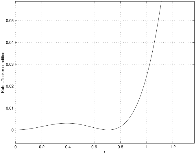
Figure 1: The Kuhn-Tucker condition for ${\sf{K}}=1$, $\alpha=0.05$ and $\kappa=10$. $F(r)=0.9\,u(r)+0.1\,u(r-1/\sqrt{2})$ and $C=0.0531$. $\lambda_{1}=0.89106$, $\lambda_{2}=0.15135$

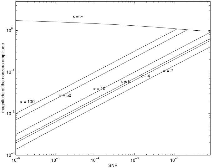
Figure 2: Location of the second mass point vs. normalized $\text{\footnotesize{SNR}}=\gamma^{2}\frac{P_{av}}{N_{0}}$ in the Rician channel ${\sf{K}}=1$.

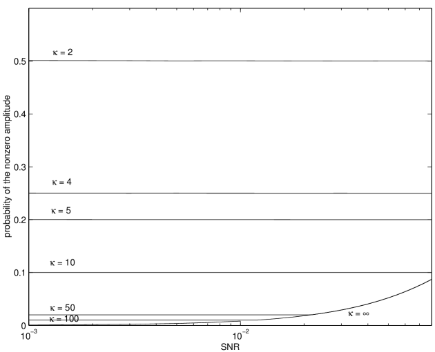
Figure 3: Probability of the second mass point vs. normalized $\text{\footnotesize{SNR}}=\gamma^{2}\frac{P_{av}}{N_{0}}$ in the Rician channel ${\sf{K}}=1$.

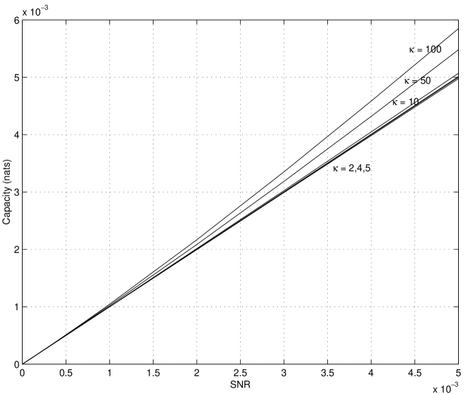
Figure 4: Capacity (in nats) vs. normalized $\text{\footnotesize{SNR}}=\gamma^{2}\frac{P_{av}}{N_{0}}$ for the Rician channel (${\sf{K}}=1$) subject to fourth moment constraints with $\kappa=2,4,5,10,50,100$.

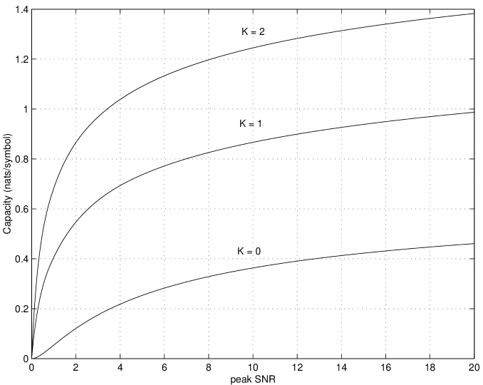
Figure 5: Capacity curves as a function of the normalized peak $\text{\footnotesize{SNR}}=\gamma^{2}\frac{P}{N_{0}}$ for the peak-power limited Rayleigh channel (${\sf{K}}=0$) and Rician channels with ${\sf{K}}=1,2$.

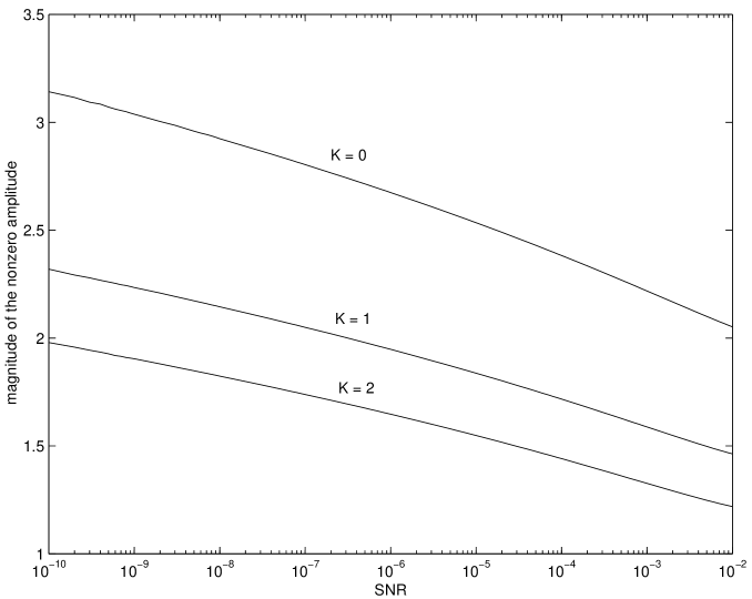
Figure 6: Magnitude of the nonzero amplitude vs. normalized $\text{\footnotesize{SNR}}=\gamma^{2}\frac{P_{av}}{N_{0}}$ for the Rician channel with phase noise ${\sf{K}}=0,1,2$.

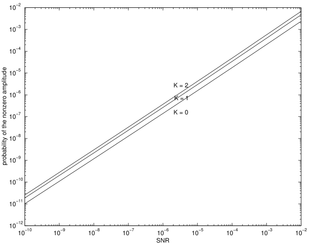
Figure 7: Probability of the nonzero amplitude vs. normalized $\text{\footnotesize{SNR}}=\gamma^{2}\frac{P_{av}}{N_{0}}$ for the Rician channel with phase noise ${\sf{K}}=0,1,2$.

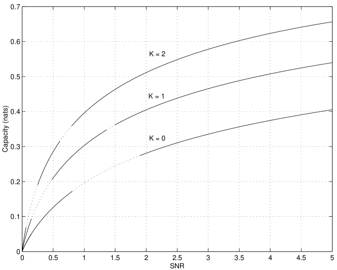
Figure 8: Capacity curves as a function of the normalized $\text{\footnotesize{SNR}}=\gamma^{2}\frac{P_{av}}{N_{0}}$ for the Rician channel with phase noise with Rician factors ${\sf{K}}=0,1,2$. The dashed segments are interpolated capacity curves. Numerical optimization methods do not provide stable results in these regions where a new mass point is emerging with a very small probability.

References

- [1] M. C. Gursoy, H. V. Poor, and S. Verdú, “The capacity of the noncoherent Rician fading channel,” Princeton University Technical Report, 2002. Available online: http://www.princeton.edu/mgursoy.
- [2] M. C. Gursoy, H. V. Poor, and S. Verdú, “The noncoherent Rician fading channel – Part II : Spectral efficiency in the low-power regime,” this issue.
- [3] S. Verdú, “Spectral efficiency in the wideband regime,” IEEE Trans. Inform. Theory, vol. 48, pp. 1319-1343, June 2002.
- [4] R. S. Kennedy, Fading Dispersive Communication Channels. Wiley Interscience, New York, 1969.
- [5] J. S. Richters,“Communication over fading dispersive channels,” Tech. Rep., MIT Research Laboratory of Electronics, Cambridge, MA, Nov. 1967.
- [6] J. G. Smith,“The information capacity of peak and average power constrained Gaussian channels,” Inform. Contr., vol. 18, pp. 203-219, 1971.
- [7] S. Shamai (Shitz) and I. BarDavid, “The capacity of average and peak-power-limited quadrature Gaussian channels,” IEEE Trans. Inform. Theory, vol. 41, pp. 1060-1071, July 1995.
- [8] I. Abou-Faycal, M. D. Trott, and S. Shamai (Shitz), “The capacity of discrete-time memoryless Rayleigh fading channels,” IEEE Trans. Inform. Theory, vol. 47, pp. 1290-1301, May 2001.
- [9] M. Katz and S. Shamai (Shitz), “On the capacity-achieving distribution of the discrete-time non-coherent and partially-coherent AWGN channels ,” submitted to IEEE Trans. Inform. Theory, 2002. See also M. Katz and S. Shamai (Shitz), “On the capacity-achieving distribution of the discrete-time non-coherent additive white Gaussian noise channel ,” Proc. 2002 IEEE Int’l. Symp. Inform. Theory, Lausanne, Switzerland, June 30 - July 5, 2002 , p. 165.
- [10] S. Shamai (Shitz), “On the capacity of a pulse amplitude modulated direct detection photon channel,” Proc. IEE, volume 137, pt. I, pages 424-430, Dec. 1990.
- [11] A. Das, “Capacity-achieving distributions for non-Gaussian additive noise channels,” Proc. 2000 IEEE Int’l. Symp. Inform. Theory, Sorrento, Italy, June 25-30, 2000, p. 432.
- [12] R. Nuriyev and A. Anastasopoulos, “Capacity characterization for the noncoherent block-independent AWGN channel,” Proc. 2003 IEEE Int’l. Symp. Inform. Theory, Yokohama, Japan, June 29 - July 4, 2003 , p. 373.
- [13] J. Huang and S. P. Meyn, “Characterization and computation of optimal distributions for channel coding,” submitted for publication. Published in abridged form in the proceedings of the 37th Annual Conference on Information Sciences and Systems, Baltimore, Maryland, March 12–14, 2003.
- [14] T. L. Marzetta and B. M. Hochwald, “Capacity of a mobile multiple-antenna communication link in Rayleigh flat fading,” IEEE Trans. Inform. Theory, vol. 45, pp. 139-157, Jan. 1999.
- [15] A. Lapidoth, “Capacity bounds via duality: a phase noise example,” Workshop on Concepts in Information Theory, Breisach, Germany, June 26-28, pp. 58-61, 2002. See also A. Lapidoth, “On phase noise channels at high SNR,” 2002 IEEE Information Theory Workshop, Bangalore, India, Oct. 20-25, pp. 1-4, 2002.
- [16] A. Lapidoth and S. M. Moser, “Capacity bounds via duality with applications to multiple-antenna systems on flat-fading channels,” IEEE Trans. Inform. Theory, vol. 49, pp. 2426-2467, Oct. 2003.
- [17] M. Médard and R. G. Gallager, “Bandwidth scaling for fading multipath channels,” IEEE Trans. Inform. Theory, vol. 48, pp. 840-852, Apr. 2002.
- [18] V. G. Subramanian and B. Hajek, “Broad-band fading channels: signal burstiness and capacity,” IEEE Trans. Inform. Theory, vol. 48, pp. 809-827, Apr. 2002.
- [19] I. E. Telatar and D. N. C. Tse, “Capacity and mutual information of wideband multipath fading channels,” IEEE Trans. Inform. Theory, vol. 46, pp. 1384-1400, July 2000.
- [20] E. Biglieri, J. Proakis, and S. Shamai (Shitz), “Fading channels: Information-theoretic and communications aspects,” IEEE Trans. Inform. Theory, vol. 44, pp. 2619-2692, October 1998.
- [21] R. Palanki, “On the capacity achieving distributions of some fading channels,” Fortieth Annual Allerton Conference on Communication, Control, and Computing, Monticello, IL, Oct. 2-4, 2002.
- [22] A. J. Goldsmith and P. P. Varaiya, “Capacity of fading channels with channel side information,” IEEE Trans. Inform. Theory, vol. 43, pp. 1986-1992, Nov. 1997.
- [23] G. Caire and S. Shamai (Shitz), “On the capacity of some channels with channel state information,” IEEE Trans. Inform. Theory, vol. 45, pp. 2007-2019, Sept. 1999.
- [24] M. Médard and A. J. Goldsmith, “Capacity of time-varying channels with channel side information,” Proc. 1997 IEEE Int’l. Symp. Inform. Theory, Ulm, Germany, June 29-July 4, 1997, p. 372.
- [25] M. Médard, “The effect upon channel capacity in wireless communications of perfect and imperfect knowledge of channel,” IEEE Trans. Inform. Theory, vol. 46, pp. 933-946, May 2000.
- [26] R. B. Ash, Information Theory. Dover: New York, 1990.
- [27] R. G. Gallager, Information Theory and Reliable Communication. Wiley: New York, 1968.
- [28] T. M. Cover and J. A. Thomas, Elements of Information Theory. Wiley: New York, 1991.
- [29] W. Rudin, Principles of Mathematical Analysis. McGraw Hill: New York, 1964.
- [30] K. Knopp, Theory of Functions. Dover: New York, 1945.
- [31] S. Lang, Complex Analysis 2nd. Ed. Springer-Verlag: New York, 1985.
- [32] G. N. Watson, A Treatise on the Theory of Bessel Functions 2nd. Ed. Cambridge University Press, 1958.