Estimation of the Number of Sources in Unbalanced Arrays via Information Theoretic Criteria

Abstract

Estimating the number of sources impinging on an array of sensors is a well known and well investigated problem. A common approach for solving this problem is to use an information theoretic criterion, such as Minimum Description Length (MDL) or the Akaike Information Criterion (AIC). The MDL estimator is known to be a consistent estimator, robust against deviations from the Gaussian assumption, and non-robust against deviations from the point source and/or temporally or spatially white additive noise assumptions. Over the years several alternative estimation algorithms have been proposed and tested. Usually, these algorithms are shown, using computer simulations, to have improved performance over the MDL estimator, and to be robust against deviations from the assumed spatial model. Nevertheless, these robust algorithms have high computational complexity, requiring several multi-dimensional searches.

In this paper, motivated by real life problems, a systematic approach toward the problem of robust estimation of the number of sources using information theoretic criteria is taken. An MDL type estimator that is robust against deviation from assumption of equal noise level across the array is studied. The consistency of this estimator, even when deviations from the equal noise level assumption occur, is proven. A novel low-complexity implementation method avoiding the need for multi-dimensional searches is presented as well, making this estimator a favorable choice for practical applications.

I Introduction

I-A Motivation

The problem of estimating the number of sources impinging on a passive array of sensors has received a considerable amount of attention during the last two decades. The first to address this problem were Wax and Kailath, [1]. In their seminal work [1] it is assumed that the additive noise process is a spatially and temporally white Gaussian random process. Given this assumption the number of sources can be deduced from the multiplicity of the received signal correlation matrix’s smallest eigenvalue [2, 3]. In order to avoid the use of subjective thresholds required by multiple hypothesis testing detectors [4], Wax and Kailath suggested the use of the Minimum Description Length (MDL) criterion for estimating the number of sources. The MDL estimator can be interpreted as a test for determining the multiplicity of the smallest eigenvalue [3].

Following [1], many other papers have addressed this problem (see, among others [5, 6, 7, 8, 9, 10]). These papers can be divided into two major groups: the first is concerned with performance analysis of the MDL estimator [11, 2, 12, 13], while the second is concerned with improvements on the MDL estimator.

Papers detailing improvements of the MDL estimator can be found quite extensively: [5, 14, 6, 15, 16, 9] is only a partial list of such works. In many of these works the MDL approach is taken, and by exploiting some type of prior knowledge, performance improvement is achieved [17, 6, 10]. One of the assumptions usually made is that the additive noise process is a spatially white process, and the robustness of the proposed methods against deviations from this assumption is usually assessed via computer simulations [9]. In general it can be observed that methods which use some kind of prior information are robust, while methods which are based on the multiplicity of the smallest eigenvalue are non-robust. The reason for these latter estimators’ lack of robustness is that, when a deviation from the assumed model occurs, the multiplicity of the smallest eigenvalue equals one [1]. Thus, one can not infer the number of sources from the multiplicity of the received signal correlation matrix’s smallest eigenvalue. On the other hand, methods that are based on some prior knowledge, e.g., the array steering vectors, usually have high computational complexity, requiring several multi-dimensional numerical searches [18]. Moreover, these methods are not necessarily consistent when some deviations from the assumed model occur, although they exhibit good robustness properties in simulations.

Efficient and robust estimation of the number of sources is very important in bio-medical applications (see, for example [19], and references therein). For example, in one such application it is of interest to estimate the number of neurons reacting to a short stimulus. This is done by placing a very large array of sensors over a patient’s head, and recording the brain activity as received by these sensors. In these bio-medical problems no a priori knowledge (e.g., knowledge of steering vectors) exists. Moreover, since different sensors are at slightly different distances from the patient’s skin, the noise levels at the outputs of the sensors vary considerably. Thus bio-medical applications are an example of one important class of problem in which the additive noise is not necessarily spatially homogeneous.

Although robust estimators for the number of sources exist, these estimators require some a priori knowledge which is often not avilable, and their computational complexity is large, as noted above. Thus, computationally efficient and robust estimators for the number of sources are of considerable interest. These estimators should not require prior knowledge and should be consistent even when deviations from the assumed model occur. Such estimators for specific types of deviations from the assumed model are developed in this paper. In particular, we consider the situation in which the sensor noise levels are spatially inhomogeneous. It will be shown that while traditional methods for estimating the number of sources tend to over-estimate the number of sources under these circumstances, our proposed estimator does not have this tendency.

I-B Problem Formulation

Consider an array of $p$ sensors and denote by ${\bf x}(t)$ the received, $p$-dimensional, signal vector at time instant $t$. Denote by $q<p$ the number of signals impinging on the array. A common model for the received signal vector is [18, 11]:

$${\bf x}(t)={\bf A}{\bf s}(t)+{\bf n}(t)\quad,\quad t=1,2,\ldots,N$$ (1)

where ${\bf A}=[{\bf a}({\bm{\psi}}_{1}),{\bf a}({\bm{\psi}}_{2}),\cdots,{\bf a}({\bm{\psi}}_{q})]$ is a $p\times q$ matrix composed of $q$ $p$-dimensional vectors, and ${\bf a}({\bm{\psi}})$ lies on the array manifold $\{{\mathcal{A}}={\bf a}({\bm{\psi}})|{\bm{\psi}}\in{\bm{\Psi}}\}$, where ${\bm{\Psi}}$ denotes a set of parameters describing the array response. ${\bf a}({\bm{\psi}})$ is called the array response vector or the steering vector and ${\bf A}$ is referred to as the steering matrix, and ${\bm{\psi}}_{i}$ is a vector of unknown parameters associated with the $i$th source. ${\bf s}(t)=[s_{1}(t)\;\cdots\;s_{q}(t)]^{T}$ is a white complex, stationary Gaussian random processes, with zero means and positive definite correlation matrix, ${\bf R}_{\bf s}$; ${\bf n}(t)$ is a temporally white complex Gaussian vector random process, independent of the signals, with zero mean and correlation matrix given by $\textnormal{diag}\left([\sigma_{1}^{2},\sigma_{2}^{2},\ldots,\sigma_{p}^{2}]\right)$, where $\textnormal{diag}\left([\sigma_{1}^{2},\sigma_{2}^{2},\ldots,\sigma_{p}^{2}]\right)$ denotes a diagonal matrix with the vector $[\sigma_{1}^{2},\sigma_{2}^{2},\ldots,\sigma_{p}^{2}]$ on its diagonal. This correlation matrix represents the scenario in which each sensor potentially faces a different noise level. Define $\sigma^{2}=\frac{1}{p}\sum_{i=1}^{p}\sigma_{i}^{2}$, $w_{i}=\sigma_{i}^{2}-\sigma^{2}$, and ${\bf w}=[w_{1},w_{2},\ldots,w_{p}]$. The additive noise correlation matrix can be described with the aid of $\sigma^{2}$ and ${\bf w}$ as follows $E\left\{{\bf n}(t){\bf n}^{H}(t)\right\}=\sigma^{2}{\bf I}+\textnormal{diag}\left({\bf w}\right)$. This alternate representation simplifies some of the proofs and derivations in the sequel. Note, that the vector ${\bf w}$ represents a deviation from the assumption that the noise level is constant across the array. Finally, all the elements of the steering matrix, ${\bf A}$, are assumed to be unknown [1], with the only restriction being that ${\bf A}$ is of full rank. In the sequel the Gaussian assumption will be eased.

We denote by ${\bm{\theta}}_{q}$ the set of unknown parameters assuming $q$ sources, that is ${\bm{\theta}}_{q}=[{\bf R}_{{\bf s},q},{\bf A}_{q},\sigma^{2}_{n,q},{\bf w}_{q}]$, where ${\bf R}_{{\bf s},q}$ is the transmitted signals’ correlation matrix assuming $q$ sources; ${\bf A}_{q}$ is the steering matrix assuming $q$ sources; $\sigma^{2}_{n,q}$ is the white noise level; and ${\bf w}_{q}$ is the vector containing the parameters representing the deviations from the spatially white noise assumption. The parameter space of the unknown parameters given $q$ sources is denoted by ${\bm{\Theta}}_{q}$. The problem is to estimate $q$ based on $N$ independent snapshots of the array output, ${\bf x}_{1}={\bf x}(t_{1}),\ldots,{\bf x}_{N}={\bf x}(t_{N})$ [1].

I-C Information Theoretic Criteria and MDL Estimators

An Information Theoretic Criterion (ITC) is an estimation criterion for choosing between several competing parametric models [3]. Given a parameterized family of probability densities, $f_{{\bf X}}\left({\bf X}|{\bm{\theta}}_{q}\right),\;{\bm{\theta}}_{q}\in{\bm{\Theta}}_{q}$ for ${\bf X}=[{\bf x}_{1},\ldots,{\bf x}_{N}]$ and for various $q$, an ITC estimator selects $\hat{q}$ such that [3]:

$$\hat{q}_{\rm ITC}=\arg\min_{q}{\rm ITC}(q)=\arg\min_{q}\left\{-L\left(\hat{\bm{\theta}}_{q}\right)+{\rm penalty}(q)\right\}$$ (2)

where $L\left({\bm{\theta}}_{q}\right)\stackrel{{\scriptstyle\triangle}}{{=}}\log f_{{\bf X}}\left({\bf X}|{\bm{\theta}}_{q}\right)$ is the log-likelihood of the measurements, $\hat{\bm{\theta}}_{q}=\arg\max_{{\bm{\theta}}_{q}\in{\bm{\Theta}}_{q}}f_{{\bf X}}\left({\bf X}|{\bm{\theta}}_{q}\right)$ is the maximum likelihood (ML) estimate of the unknown parameters given the $q$th family of distributions, and ${\rm penalty}(q)$ is some general penalty function associated with the particular ITC used. The MDL and AIC estimators are given by ${\rm penalty}(q)=0.5|{\bm{\Theta}}_{q}|\log\left(N\right)$ and ${\rm penalty}(p)=|{\bm{\Theta}}_{q}|$ respectively, where $|{\bm{\Theta}}_{q}|$ is the number of free parameters in ${\bm{\Theta}}_{q}$ [20, 21, 1]. It is well known that, asymptotically and under certain regularity conditions, the MDL estimator minimizes the description length (measured in bits) of both the measurements, ${\bf X}$, and the model, $\hat{\bm{\theta}}_{q}$ [22], while the AIC criterion minimizes the Kullback-Liebler divergence between the various models and the true one. In the rest of the paper we will consider only the MDL criterion, although other penalty functions can also be treated similarly.

Although in many problems associated with array processing, e.g., direction of arrival (DOA) estimation, one has some prior knowledge about the array structure, when estimating the number of sources this prior knowledge is usually ignored [1, 18]. The reason for this is that by ignoring the array structure and assuming Gaussian signals and noise, and ${\bf w}\equiv\bf 0$, the resulting MDL estimator (2), termed here the Gaussian-MDL (GMDL) estimator [11], has a simple closed form expression given by [1]

$$\hat{q}|_{{\rm GMDL}}=\arg\min_{q=0,\ldots,p-1}\left[-N\log\frac{\prod_{i=q+1}^{p}l_{i}}{\left(\frac{1}{p-q}\sum_{i=q+1}^{p}l_{i}\right)^{p-q}}\right.$$

$$+\left.\frac{1}{2}(q(2p-q)+1)\log N\right]$$ (3)

where $l_{1}\geq l_{2}\geq\cdots\geq l_{p}$ are the eigenvalues of the empirical received signal’s correlation matrix, $\widehat{\bf R}=\frac{1}{N}\sum{\bf x}_{i}{\bf x}_{i}^{H}$. It is well known that when ${\bf w}\equiv\bf 0$ the GMDL estimator is a consistent estimator of the number of sources, while when ${\bf w}\neq 0$, the GMDL estimator, (3), is not consistent and in fact, as the number of snapshots approaches infinity, the probability of error incurred by the GMDL estimator approaches one [11].

Denote by ${\bf\mathcal{R}}_{q}$ the set of all positive definite, rank $q$, Hermitian, $p\times p$ matrices, and by ${\bf\mathcal{W}}$ the set of all zero mean $p$-length vectors. Given the assumptions made in the problem formulation, the MDL estimator for estimating the number of sources, denoted hereafter as the Robust-MDL (RMDL) estimator, is given by,

$$\hat{q}_{{\rm RMDL}}=\arg\min_{q=0,\ldots,p-1}$$

$$\left\{N\log\left|\hat{{\bf A}}_{q}\hat{{\bf R}}_{{\bf s},q}\hat{{\bf A}}^{H}_{q}+\hat{\sigma}^{2}_{n,q}{\bf I}+\textnormal{diag}\left(\hat{{\bf w}}_{q}\right)\right|\right.$$

$$\left.+{\rm Tr}\left\{\left(\hat{{\bf A}}_{q}\hat{{\bf R}}_{{\bf s},q}\hat{{\bf A}}^{H}_{q}+\hat{\sigma}^{2}_{n,q}{\bf I}+\textnormal{diag}\left(\hat{{\bf w}}_{q}\right)\right)^{-1}\hat{{\bf R}}\right\}\right.$$

$$+\left.\frac{1}{2}(q(2p-q)+p)\log N\right\}$$ (4)

where $\hat{{\bf A}}_{q},\hat{{\bf R}}_{{\bf s},q},\hat{\sigma}^{2}_{n,q},\hat{{\bf w}}_{q}$ are the ML estimates of the unknown parameters assuming $q$ sources, that is

$$\hat{{\bf A}}_{q},\hat{{\bf R}}_{{\bf s},q},\hat{\sigma}^{2}_{n,q},\hat{{\bf w}}_{q}=\arg\max_{{\bf A}_{q}{\bf R}_{{\bf s},q}{\bf A}_{q}^{H}\in{\bf\mathcal{R}}_{q},\sigma^{2}_{n,q}>0,{\bf w}_{q}\in{\bf\mathcal{W}}}$$

$$\left[-N\log\left|{\bf A}_{q}{\bf R}_{{\bf s},q}{\bf A}^{H}_{q}+\sigma^{2}_{n,q}{\bf I}+\textnormal{diag}\left({\bf w}_{q}\right)\right|\right.$$

$$\left.+{\rm Tr}\left\{\left({\bf A}_{q}{\bf R}_{{\bf s},q}{\bf A}^{H}_{q}+\sigma^{2}_{n,q}{\bf I}+\textnormal{diag}\left({\bf w}_{q}\right)\right)^{-1}\hat{{\bf R}}\right\}\right].$$ (5)

Note that since ${\bf A}_{q}{\bf R}_{{\bf s},q}{\bf A}_{q}^{H}\in{\bf\mathcal{R}}_{q}$, by using eigen-decomposition we can write ${\bf A}_{q}{\bf R}_{{\bf s},q}{\bf A}_{q}^{H}=\sum_{i=1}^{q}\lambda_{i}{\bf v}_{i}{\bf v}_{i}^{H}$, where $\{{\bf v}_{i}\}$ is an orthonormal set of vectors. Hence, the vector of unknown parameters assuming $q$ sources is also given by

$${\bm{\theta}}_{q}=[\lambda_{1},\ldots,\lambda_{q},{\bf v}_{1}^{T},\ldots,{\bf v}_{q}^{T},{\bf w}^{T},\sigma_{n}^{2}].$$ (6)

I-D Organization of the Paper

The rest of this paper is organized as follows: In Section II we discuss the indentifiabilty of the estimation problem and we prove the consistency of the RMDL estimator. In Section III we describe a low-complexity algorithm for approximating the RMDL estimator, (4), and we discuss the properties of this algorithm. In Section IV we present empirical results. In Section V some concluding remarks are provided.

II Identifiability and Consistency of the RMDL Estimator

II-A Identifiability

Consider a parameterized family of probability density functions (pdf’s) $f_{{\bf X}}({\bf x}|{\bm{\theta}}),\;{\bm{\theta}}\in{\bm{\Theta}}$. This family of densities is said to be identifiable if for every ${\bm{\theta}}\neq{\bm{\theta}}^{\prime}$, the Kullback-Liebler divergence between $f_{{\bf X}}\left({\bf x}|{\bm{\theta}}\right)$ and $f_{{\bf X}}\left({\bf x}|{\bm{\theta}}^{\prime}\right)$ is greater than zero, that is $D\left(f_{{\bf X}}\left({\bf x}|{\bm{\theta}}\right)||f_{{\bf X}}\left({\bf x}|{\bm{\theta}}^{\prime}\right)\right)>0$, where $D(f({\bf x})||g({\bf x}))=\int f\log\frac{f}{g}$ is the Kullback-Leibler divergence between $f({\bf x})$ and $g({\bf x})$ [23]. This condition insures that there is a one-to-one relationship between the parameter space and the statistical properties of the measurements.

The problem discussed in Section I-B is a model order selection problem [22]. This problem is unidentifiable if it is possible to find for some $k\neq l$ two points in the parameter space, ${\bm{\theta}}_{k}\in{\bm{\Theta}}_{k}$ and ${\bm{\theta}}_{l}\in{\bm{\Theta}}_{l}$ such that $f\left(\cdot|{\bm{\theta}}_{k}\right)=f\left(\cdot|{\bm{\theta}}_{l}\right)$. Unfortunately, we can, in fact, identify two such points leading to the conclusion that the estimation problem discussed in Section I-B is unidentifiable. The received signal’s pdf is fully characterized by the received signal’s correlation matrix. Thus, in order to prove that the problem is unidentifiable, it suffices to find two different parameter values under which the corresponding received signal’s correlation matrices are equal. Take, for example, the following received signal correlation matrix: $\textnormal{diag}\left([11,10.5,9.5,10]\right)$. This correlation matrix can result from a noise-only scenario with $\sigma_{n}^{2}=10.25$ and ${\bf w}=[0.75,0.25,-~{}0.75,-~{}0.25]$, or from a one source scenario where $\sigma_{n}^{2}=10,{\bf w}=[0,0.5,-~{}0.5,0],{\bf a}=[1,0,0,0]^{T}$, and ${\bf R}_{{\bf s}}=1$. Thus we have found two scenarios, the first corresponding to a noise only scenario, and the other corresponding to a one source scenario, such that the distribution of the received signal vector is the same. Thus, this example shows that the estimation problem formulated is unidentifiable.

In order to make the estimation problem identifiable, all the points having the same received signal pdf must be removed from the parameter space except one. As is the custom in model order selection problems, among all the points having the same received signal pdf, the one with the smallest number of sources, that is, the point with the lowest number of unknown parameters, is left in the parameter space, and the remaining ones are deleted. The main question that arises is whether most of the points in the parameter space are identifiable or not. Fortunately, the answer to this question is yes; that is, most of the points in the parameter space are identifiable. The following lemma characterizes all the unidentifiable points in the parameter space.

Lemma 1

Suppose $q<p$. Then ${\bm{\theta}}_{q}$ is an unidentifiable point in the parameter space if and only if the matrix $\sum_{i=1}^{q}{\bf v}_{i}{\bf v}_{i}^{H}$ contains $\alpha{\bf e}_{j}=[{\bf 0}_{j-1},1,{\bf 0}_{p-j}]$ as its $j$th row for some $j\in[1,\ldots,p]$, where ${\bf v}_{i}$ defined in (6).

Proof of Lemma 1

See Appendix A

The proof of Lemma 1 provides an interesting physical interpretation of the unidentifiable points. In particular, it can be seen from the proof of the lemma that all the unidentifiable points are similar to the above example used to show that the problem is unidentifiable. That is, an unidentifiable point corresponds to a scenario where there are, say $q$ sources, and one of them is received at only one of the sensors. Since this source can not be distinguished from a deviation, from some nominal value, of the noise level in the corresponding element, this scenario could be confused with a different scenario having one fewer source, and an increase in the noise level at the proper element. From a practical viewpoint, this type of situation is a rarity.

II-B Consistency of the RMDL Estimator

In the previous subsection it was proved that the estimation problem defined in Section I-B is unidentifiable. Nevertheless, it was also argued that only a small portion of the points in the parameter space are unidentifiable, meaning that by excluding these points from the parameter space the problem becomes identifiable. For the rest of this paper, we consider these points to be excluded from the parameter space. Once the estimation problem has been shown to be identifiable, it is possible to infer the number of sources from the measurements. However for a specific estimator, the issue of consistency must be considered.

In model order selection, the common performance measure is the probability of error, that is $P_{e}={\rm P}\left(\hat{q}\neq q\right)$ [3]. In what follows the RMDL estimator, (4), is proven to be a consistent estimator, that is $\lim_{N\rightarrow\infty}P_{e}=0$.

Lemma 2

The RMDL estimator, (4), is a consistent estimator of the number of sources.

Proof of Lemma 2

See Appendix B

Deviations from the assumption of spatial homogeneity are part of our general model. Thus, even if the noise levels at various sensor are not equal, according to Lemma 2 the RMDL estimator, (4), is still consistent. That is, the probability of error of the RMDL estimator still converges to zero even in the presence of deviations from assumption of equal noise levels.

It is well known that the GMDL estimator, (3), is a non-robust estimator when the noise levels at the various sensor are not equal, i.e., the probability of error of the GMDL estimator approaches one as $N\rightarrow\infty$. Nevertheless, it is known that the GMDL estimator is robust against statistical mismodeling. Under very weak regularity conditions, if the transmitted signal and/or the additive noise are non-Gaussian, then the probability of error of the GMDL estimator still converges to zero. Fortunately, it can be shown that the RMDL estimator, (4) is robust against statistical mismodeling as well. Being robust against both statistical and spatial mismodeling is an advantage of the RMDL estimator over the GMDL estimator.

We conclude this subsection by proving that the RMDL estimator, (4) is a consistent estimator even in the presence of statistical mismodeling. Denote by $g({\bf x})$ the actual pdf of the received signal at some time instant, and by $f\left({\bf x}|{\bm{\theta}}\right)$ the assumed measurement pdf, i.e., the Gaussian distribution. Note that it is still assumed that ${\bf R}_{\bf x}=E\left\{{\bf x}{\bf x}^{H}\right\}$ has the following form ${\bf R}_{\bf x}={\bf A}_{\bf s}{\bf R}_{\bf s}{\bf A}^{H}+\sigma_{n}^{2}{\bf I}+\textnormal{diag}\left({\bf w}\right)$. Let ${\rm E}_{g}\left\{h({\bf x})\right\}=\int h({\bf x})g({\bf x}){\rm d}{\bf x}$. The following lemma establishes the consistency of the RMDL estimator when the sources are not Gaussian

Lemma 3

Assume that ${\rm E}_{g}\left\{\frac{\partial\log f\left({\bf x}|{\bm{\theta}}\right)}{\partial{\bm{\theta}}}\frac{\partial\log f\left({\bf x}|{\bm{\theta}}\right)}{\partial{\bm{\theta}}}^{T}\right\}$ and ${\rm E}_{g}\left\{\frac{\partial^{2}\log f\left({\bf x}|{\bm{\theta}}\right)}{\partial{\bm{\theta}}(\partial{\bm{\theta}})^{T}}\right\}$ exist and are finite. Then the probability of error of the RMDL estimator converges to zero as $N\rightarrow\infty$.

Proof of Lemma 3

See Appendix C.

III A Practical Estimation Algorithm

In the previous section the asymptotic properties of the RMDL estimators were considered. It was proven that the RMDL estimator is both a consistent and robust estimator of the number of sources. These two properties make the RMDL estimator very appealing for use in practical problems. However the computational complexity of the RMDL estimator is still very high compared to that of the GMDL estimator. Recall that in order to implement the RMDL estimator ML estimates of the unknown parameters must be found for every possible number of sources. Since no closed-form expression for these ML estimates exists, multi-dimensional numerical searches must be used in order to find them. Even for moderate array sizes, e.g., $p=6$, the number of unknown parameters is a few dozen, which makes the task of finding the ML estimates impractical.

In order to overcome the computational burden of computing the ML estimates, we propose to replace the ML estimates by estimates obtained using a low-complexity estimation algorithm. A reasonable criterion used in array processing applications is to choose as an estimate the parameter vector that minimizes the Frobenius norm of the error matrix [24, 25]; that is

$$\hat{{\bm{\theta}}}_{q,LS} = \arg\min_{{\bm{\theta}}_{q}\in{\bm{\Theta}}_{q}}||(\widehat{\bf R}-{\bf R}_{\bf x}({\bm{\theta}}_{q}))||_{F}^{2}$$ (7)

$$= \arg\min_{{\bm{\theta}}_{q}\in{\bm{\Theta}}_{q}}{\rm Tr}\left\{(\widehat{\bf R}-{\bf R}_{\bf x}({\bm{\theta}}_{q}))(\widehat{\bf R}-{\bf R}_{\bf x}({\bm{\theta}}_{q}))^{H}\right\}$$

$$= \arg\min_{{\bm{\theta}}_{q}\in{\bm{\Theta}}_{q}}\sum_{i=1}^{p}\sum_{j=1}^{p}\left|[(\widehat{\bf R}-{\bf R}_{\bf x}({\bm{\theta}}_{q}))(\widehat{\bf R}-{\bf R}_{\bf x}({\bm{\theta}}_{q}))]_{ij}\right|^{2}$$

and the corresponding estimate for the number of sources is given by,

$$\hat{q}=\arg\min_{q=0,\ldots,p-1}\left[-L\left(\hat{\bm{\theta}}_{q,LS}\right)+q(2p-q)\frac{\log N}{2}\right].$$ (8)

Replacing the ML estimates with their LS counterparts raises two important questions. One is whether replacing the ML estimates with the LS estimates results in performance loss; and the second is whether efficient algorithms for computing the LS estimates exist. Fortunately, it can be demonstrated that no performance loss is incurred (asymptotically) by replacing the ML estimates with the LS estimates, and an efficient algorithm for computing the LS estimates exists. It was pointed out by one of the reviewers that for finite sample sizes since the ML estimates are replaced by the LS estimates, it is not guaranteed that $L\left(\hat{\bm{\theta}}_{q,LS}\right)<L\left(\hat{\bm{\theta}}_{q+1,LS}\right)$. This problem can be easily solved by noting that because the problem is a nested hypotheses problem $hat{\theta}_{q}\in\Theta_{q+1}$. Therefore, if $L(\hat{\theta}_{q|LS})<L(\hat{\theta}_{q+1|LS})$, we can use $L(\hat{\theta}_{q|LS})$ instead of $L(\hat{\theta}_{q+1|LS})$ in the MDL formula.

Our problem is a model order selection problem, and our main interest is in the probability of error of the proposed estimator. In [11], it is demonstrated that the MDL’s asymptotic probability of error depends on ${\bm{\theta}}_{q}$ and ${\bm{\theta}}_{q-1}^{\ast}\in{\bm{\Theta}}_{q-1}$, where ${\bm{\theta}}_{q-1}^{\ast}=\arg\min_{{\bm{\theta}}_{q-1}}D(f({\bf x}|{\bm{\theta}}_{q})||f({\bf x}|{\bm{\theta}}_{q-1}))$. It is easily seen that ${\bm{\theta}}_{q-1}^{\ast}$ is the limit of the ML estimates under the assumption of $q-1$ sources, i.e., $\hat{{\bm{\theta}}_{q-1}}|{\bm{\theta}}_{q}\stackrel{{\scriptstyle N\rightarrow\infty}}{{\longrightarrow}}{\bm{\theta}}_{q-1}^{\ast}$. Analysis similar to that in [11] demonstrates that if a consistent estimator is used instead of the ML estimator in the MDL estimator, then the asymptotic probability of detection remains the same. Since the LS estimator is a consistent estimator of the unknown parameters, the asymptotic performance of the RMDL’s simplified version, (8), is the same as the asymptotic performance of the RMDL estimator, (4).

Similarly to the ML estimates, $\hat{{\bm{\theta}}}_{q,LS}$ is the solution of a nonlinear programming problem, requiring brute-force multi-dimensional search. Nevertheless, based on the concept of serial interference cancellation (SIC) [26], in what follows a novel algorithm for finding $\hat{{\bm{\theta}}}_{q,LS}$ is suggested. In this algorithm the unknown parameters are divided into two groups, and given the estimate of one group of unknown parameters, an estimate of a second group of unknown parameters is constructed. The estimates are constructed in such a way as to insure a decrease in the Frobenius norm of the error matrix after each iteration. The estimation process iterates between the two groups of unknown parameters, until the estimates converge to a stationary point.

In multiple access communications two (or more) users transmit information over two non-orthogonal subspaces. The serial interference cancellation multiuser detection algorithm for data detection in such situations works as follows. First, the unknown parameters associated with the first user are estimated. Next, an error signal is constructed by subtracting from the received signal the estimated first user’s transmitted signal. In the next stage, the unknown parameters associated with the second user are estimated from the error signal. In the next iteration, the unknown parameters associated with the first user are re-estimated based on the received signal after subtraction of the estimated second user’s transmitted signal. This iterative process is continued until convergence is reached.

The principle behind the SIC multiuser detector can be used for constructing a novel low-complexity estimation algorithm for estimating the unknown parameters in the present situation. In what follows such a low-complexity estimation algorithm is described and its properties are discussed. The unknown parameters in our estimation problem are $[\lambda_{1},\ldots,\lambda_{q},{\bf v}_{1}^{T},\ldots,{\bf v}_{q}^{T},{\bf w}^{T},\sigma_{n}^{2}]$, or equivalently, ${\bf A}_{q}{\bf R}_{{\bf s},q}{\bf A}_{q}^{H},\sigma_{n,q}^{2},{\bf w}_{q}$. These unknown parameters are divided into two groups. The first group contains $[\lambda_{1},\ldots,\lambda_{q},{\bf v}_{1}^{T},\ldots,{\bf v}_{q}^{T},\sigma_{n}^{2}]$, or equivalently ${\bf A}_{q}{\bf R}_{{\bf s},q}{\bf A}_{q}^{H}$ and $\sigma_{n,q}^{2}$, while the second contains ${\bf w}_{q}$. The first group corresponds to the unknown parameters of the ideal point source plus spatially white additive noise model, while the second corresponds to the unknown parameters representing the deviations from the ideal model. In a sense, ${\bf w}_{q}$ can be regarded as the unknown parameters that robustify the estimator. The input to the algorithm is $\widehat{\bf R}_{\bf x}=\frac{1}{N}\sum_{t=1}^{N}{\bf x}(t_{i}){\bf x}(t_{i})^{H}$ which is a sufficient statistic for estimating the unknown parameters, assuming Gaussian sources and noise.

Denote by $\sigma_{n,q}^{j},{\bf A}_{q}^{j}{\bf R}_{{\bf s},q}^{j}\left({\bf A}_{q}^{j}\right)^{H}$, and ${\bf w}_{q}^{j}$ the estimates of the unknown parameters after the $j$th iteration. The proposed algorithm is implemented as follows: In the first iteration, $\sigma_{n,q}^{1},{\bf A}_{q}^{1}{\bf R}_{{\bf s},q}^{1}\left({\bf A}_{q}^{1}\right)^{H}$ are estimated from $\widehat{\bf R}_{\bf x}$. The best estimates, in both the ML sense and the Least Squares (LS) sense (see appendix D), are

$$\sigma_{n,q}^{1}=\sqrt{\frac{1}{p-q}\sum_{i=q+1}^{p}l_{i}}$$ (9)

$${\bf A}_{q}^{1}{\bf R}_{{\bf s},q}^{1}\left({\bf A}_{q}^{1}\right)^{H}=\sum_{i=1}^{q}\left(l_{i}-\left(\sigma_{n,q}^{1}\right)^{2}\right){\bf v}_{i}{\bf v}_{i}^{H}$$ (10)

where $l_{1}>\cdots>l_{p}$ and ${\bf v}_{1},\ldots,{\bf v}_{p}$ are, respectively, the eigenvalues and eigenvectors of $\widehat{\bf R}_{\bf x}$. In the next step an error matrix, denoted by ${\bf E}$, is constructed by subtracting from $\widehat{\bf R}_{\bf x}$ the estimate for the estimated part of the received signal’s correlation matrix corresponding to the ideal model, that is ${\bf A}_{q}^{1}{\bf R}_{{\bf s},q}^{1}\left({\bf A}_{q}^{1}\right)^{H}+\left(\sigma_{n,q}^{1}\right)^{2}{\bf I}$. Thus, the error matrix is given by

$${\bf E}=\widehat{\bf R}-{\bf A}_{q}^{1}{\bf R}_{{\bf s},q}^{1}\left({\bf A}_{q}^{1}\right)^{H}-\left(\sigma_{n,1}^{1}\right)^{2}{\bf I}.$$ (11)

Next, ${\bf w}_{q}^{1}$ is estimated from ${\bf E}$, and the best estimate in both the ML and LS sense is,

$${\bf w}_{q}^{1}=\textnormal{diag}\left({\bf E}\right).$$ (12)

At the $j$th iteration, we apply the same procedure except that $\sigma_{n,q}^{j}$ and ${\bf A}_{q}^{j}{\bf R}_{{\bf s},q}^{j}\left({\bf A}_{q}^{j}\right)^{H}$ are estimated from $\widehat{\bf R}-{\bf w}_{q}^{j-1}$, while ${\bf w}_{q}^{j}$ is estimated from $\widehat{\bf R}-{\bf A}_{q}^{j}{\bf R}_{{\bf s},q}^{j}\left({\bf A}_{q}^{j}\right)^{H}-\left(\sigma_{n,q}^{j}\right)^{2}{\bf I}$.

Summarizing the above, our proposed estimation algorithm is given as follows:

1. Initialize ${\bf E}=\widehat{\bf R}$.

2. Compute $l_{1}\geq\cdots l_{p}$, ${\bf v}_{1},\ldots,{\bf v}_{p}$ the eigenvalues and the corresponding eigenvectors of ${\bf E}$.

3. Compute the following estimates,

   $$\sigma_{n,q}=\sqrt{\frac{1}{p-q}\sum_{i=q+1}^{p}l_{i}}$$ (13)

   $${\bf A}_{q}{\bf R}_{{\bf s},q}\left({\bf A}_{q}\right)^{H}=\sum_{i=1}^{q}\left(l_{i}-\left(\sigma_{n,q}\right)^{2}\right){\bf v}_{i}{\bf v}_{i}^{H}$$ (14)

   $${\bf w}_{q}=\textnormal{diag}\left(\widehat{\bf R}-{\bf A}_{q}{\bf R}_{{\bf s},q}\left({\bf A}_{q}\right)^{H}-\left(\sigma_{n,q}\right)^{2}{\bf I}\right)$$ (15)

4. Compute ${\bf E}=\widehat{\bf R}-{\bf w}_{q}$.

5. If the estimates have stabilized, stop; otherwise return to step 2.

A major question that arises is whether this algorithm is guaranteed to converge and, if so, whether the stationary point of the algorithm is optimal in some sense. Fortunately, the answers to these questions are yes. In Appendix D it is proven that in each step of the algorithm, the Frobenius norm of the error matrix decreases, that is $||\widehat{\bf R}-{\bf R}({\bm{\theta}}_{q}^{n})||_{F}^{2}\geq||\widehat{\bf R}-{\bf R}({\bm{\theta}}_{q}^{n+1})||_{F}^{2}$, where ${\bm{\theta}}_{q}^{n}$ is the estimate of the unknown parameters after the $n$th iteration. This also proves that the proposed algorithm converge to a local minimum of the LS cost function.

Consider our proposed iterative algorithm. The most complex operation in our algorithm is the eigenvalue decomposition whose complexity is ${\mathcal{O}}(p^{3})$. Since the process is repeated $p$ times (one for each possible number of sources), the complexity of our algorithm is ${\mathcal{O}}(p^{4})$ per iteration.

Since no closed expression for the ML estimates exists, some numerical maximization method must be used. Therefore, the complexity of the ML estimator depends on the number of iterations and the exact numerical maximization method used. However, we can still demonstrate that the complexity of the ML estimator is higher than that of our proposed algorithm. Since efficient numerical maximization algorithms require the computation of the derivative of the likelihood function, we examine the complexity of computing this derivative. The most complex operation in computing the derivative is $\frac{\partial{\rm Tr}\left\{{\bf R}_{{\bf x}}^{-1}({\bm{\theta}})\widehat{\bf R}\right\}}{\partial\theta_{i}}=-{\rm Tr}\left\{\left[{\bf R}_{{\bf x}}^{-1}({\bm{\theta}})\widehat{\bf R}{\bf R}_{{\bf x}}^{-1}({\bm{\theta}})\right]\frac{\partial{\bf R}_{{\bf x}}^{-1}({\bm{\theta}})}{\partial\theta_{i}}\right\}$, which has a complexity of ${\mathcal{O}}(p^{8})$. This operation has to be repeated $p$ times, one for each possible number of sources. Therefore the complexity of computing the derivative of the likelihood function per iteration is ${\mathcal{O}}(p^{9})$. It follows that for $p>3$, the complexity of the ML estimator is higher by several orders of magnitude than our proposed iterative algorithm.

IV Simulations

In this subsection simulation results with synthetic data are presented. We consider a uniform linear array with 10 elements, and assume three equal-power and independent sources having signal-to-noise ratio (SNR) per element of $0\;dB$. The sources’ directions of arrival (DOA’s) are taken to be $[0^{\circ}\;5.7^{\circ}\;11.4^{\circ}]$. We consider two cases: the first corresponds to complex Gaussian sources, i.e., $s(t)\sim{\mathcal{C}N}\left(0,\sigma^{2}\right)$; and the second corresponds to sources that are distributed as complex Laplacian sources, i.e., $\Re\left(s(t)\right)$ and $\Im\left(s(t)\right)$ are independent random variables having pdf $\frac{1}{\alpha}e^{-\frac{|x|}{\alpha}}$. The second case corresponds to impulsive sources usually found in bio-medical application.

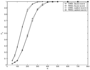
Figure 1: Three-user scenario, no mismatch. Probability of correct decision as a function of the number of snapshots.

We first consider the case in which ${\bf w}=0$; i.e., the noise is spatially white. Figure 1 depicts the probability of correct decision in this case of both the GMDL estimator and the RMDL estimator when used with the estimates computed by the iterative algorithm. Since no deviations from the spatial white noise model exist in this case, the GMDL estimator is both consistent and robust, and indeed the empirical probability of error of the GMDL estimator converges to zero whether the sources are Gaussian or Laplacian. The RMDL estimator is also both a consistent and a robust estimator, and again the empirical probability of error of the RMDL estimator converges to zero as well, independent of the source distribution. These empirical results demonstrate that the GMDL estimator is superior to the RMDL estimator in this situation, an additional 100 samples are required by the RMDL estimator in order to achieve the same probability of correct decision as the GMDL estimator. In [27] it was proven that by exploiting more prior information the performance of the MDL estimator improves. This explains the superiority of the GMDL estimator over the RMDL estimator, since the GMDL estimator makes use of the spatial whiteness of the additive noise process, while the RMDL estimator ignores this information.

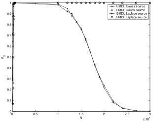
Figure 2: Three-user scenario, weak mismatch. Probability of correct decision as a function of the number of snapshots.

In practice, multi-channel receivers are used in DOA estimation systems. The noise level in each receiver is different and hence the system has to be calibrated. Due to finite integration time, errors and different drifts in each channel, small differences in the noise levels at the different receiver channels exist. In the next example this scenario is simulated. For simulating this scenario ${\bf w}$ is taken to be ${\bf w}=\frac{\sigma_{n}^{2}}{10}[-9/10,-7/10,\ldots,9/30]$. This ${\bf w}$ represents a scenario in which the noise level in each receiver is different from the nominal noise level by no more than $-10\,dB$. Figure 2 depicts the probability of correct decision of both the GMDL and the RMDL estimators as functions of the number of snapshots taken for both Gaussian and Laplacian sources.

The multiplicity of the received signal correlation matrix’s smallest eigenvalue is equal to one, and hence the GMDL estimator is not consistent, that is ${\rm P}\left(\hat{q}\neq 3\right)\rightarrow 1$ [3]. From Fig. 2 it is seen that the empirical probability of error of the GMDL estimator converges to one as the number of snapshots increases. Nevertheless, it can be seen that this happen only when the number of snapshots is quite large (about 10,000). This phenomenon can be explained by examining the eigenvalues of the received signal’s correlation matrix. The eigenvalues of the received signal’s correlation matrix are given by $[20.1,10.9,1.93,1.07,\cdots,0.92]$. For the GMDL estimator, the simulated scenario corresponds to a scenario where $p-1$ sources exists, the noise level equals to $0.9$, and the SNR of the fourth strongest source at the array output is $-7\,dB$. The GMDL requires about 10,000 snapshots in order for the probability of detection of this weak “virtual” source to be noticeable. As the number of snapshots increases, the probability of detection of this weak virtual source increases as well, causing the probability of correct decision to decrease to zero. On the other hand, it can be seen that the probability of error of the RMDL estimator converges to zero as the number of snapshots increases for both the Gaussian and the Laplacian sources. This demonstrate both the consistency and the robustness of the RMDL estimator.

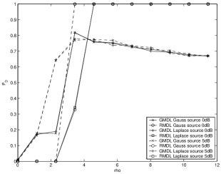
Figure 3: Three-user scenario, weak mismatch. Probability of correct decision as a function of the spatial separation between the sources.

In Figure 3 we study the spatial separation between the sources required for reliable detection. We assume that the three sources’ directions of arrival are $[0,\rho,2\rho]$, 15,000 snapshots are taken by the receiver, and the SNR per element is either $0\,dB$ or $5\,dB$. Figure 3 depicts the probability of correct decision of both the GMDL and the RMDL estimators for both Gaussian and Laplacian sources as a function of $\rho$.

In the figure we can see again that the RMDL estimator outperforms the GMDL estimator. Even if large separation between the sources exists, the probability of correct decision of the GMDL estimator does not approach one. The probability of correct decision of the RMDL estimator, on the other hand, approaches one with the increase in the separation between the sources. This difference can be explained with the aid of the received signal correlation matrix’s eigenvalue spectrum. The received signal correlation matrix eigenvalues equal $[11.54,11.05,10.39,1.07,...,0.9237]$. The three highest eigenvalues correspond to the three sources. However, due to the different noise level in each sensor, the rest of the eigenvalues are not equal to the noise level. The large number of snapshots enables the GMDL estimator to detect the differences in the weakest eigenvalues as valid sources, which results in an error event. However, if the number of snapshots is reduced, the GMDL estimator will not detect these differences. Nonetheless, if the number of snapshot is reduced, and a valid weak source exists, the GMDL estimator will not detect this valid source.

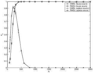
Figure 4: Three-user scenario, strong mismatch. Probability of correct decision as a function of the number of snapshots.

As discussed in the beginning of this paper, in biological applications the noise level may vary considerably between the different receiver channels. Thus, large deviations from the ideal model are expected in such systems. For simulating this type of scenario we take ${\bf w}=\frac{\sigma_{n}^{2}}{2}[-9/10,-7/10,\ldots,9/10]$, which represents deviations of up to $-3\,dB$ from the nominal noise level. Figure 4 depicts the probabilities of correct decision of the GMDL and the RMDL estimators as functions of the number of snapshots taken.

It can be seen that in this scenario the empirical error probability of the GMDL estimator approaches one even when the number of snapshots is small (about 750). Again, this can be explained by examining the received signal correlation matrix’s eigenvalues, which are equal to $[20.13,10.93,2,1.36,\ldots,0.62]$. The GMDL estimator interprets this scenario as a $p-1$ sources scenario with the noise level equal to $0.5$, and the SNR of the fourth strongest source at the array output is $6\,dB$. Due to its high SNR, only a small number of snapshots are required for detecting this “virtual” source, and by detecting this virtual source an error event is created. As the number of snapshots increases, the probability of detection of this virtual source increases as well, causing the probability of correct decision to decrease to zero. Again, it can be seen that the probability of error of the RMDL estimator converges to zero as the number of snapshots increases.

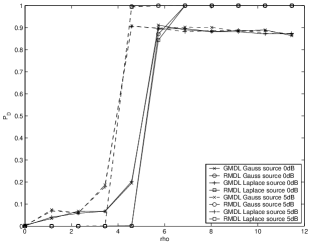
Figure 5: Three-user scenario, strong mismatch. Probability of correct decision as a function of the spatial separation between the sources

In the last figure, Figure 5, we study the spatial separation between the sources required for reliable detection when the deviation from the equal noise power assumption is large. We assume that three sources’ directions of arrival are $[0,\rho,2\rho]$, 250 snapshots are taken by the receiver, and the SNR per element is either $0\,dB$ or $5\,dB$. Figure 5 depicts the probabilities of correct decision of both the GMDL and the RMDL estimators for the Gaussian and Laplacian sources as a function of $\rho$. Again, we can see that the RMDL estimator outperforms the GMDL estimator. Even for large separation between the sources, the deviation from the equal noise level assumption results in a change in the eigenvalue structure. This change is detected by the GMDL estimator as an additional sources, and hence an error event occurs.

V Summary and Concluding Remarks

In this paper the problem of robust estimation of the number of sources impinging on an array of sensors has been addressed. It has been demonstrated that by proper use of additional unknown parameters, the resulting estimator, denoted as the RMDL estimator, is robust against both spatial and statistical mismodeling. This situation represents an improvement on the traditional MDL estimator which is robust only against statistical mismodeling. In addition, a novel low-complexity algorithm for computing the estimates of the unknown parameters has been presented. It has been shown that this algorithm converges to the LS estimates of the unknown parameters. On one hand, the computational complexity of the proposed estimator is higher than the complexity of the traditional MDL estimator; on the other hand the complexity is far less than the complexity of known robust estimators which require several multi-dimensional searches.

The proposed estimation algorithm can be used to robustify other estimation algorithms as well. Take for example the MUSIC algorithm for estimating DOAs [28]. It is well known that the MUSIC algorithm is not robust against spatial mismodeling. Even slight spatial mismodeling can cause a large error in the estimated signal subspace, leading to substantial estimation errors. The use of our estimation technique to improve the robustness of the MUSIC algorithm is an interesting topic for further study.

Appendix A Proof of Lemma 1

In this appendix Lemma 1 is proven by a way of induction on the number of sources. We first note that since $\sum_{i=1}^{q}{\bf v}_{i}{\bf v}_{i}^{H}$ is an Hermitian matrix, then if $\sum_{i=1}^{q}{\bf v}_{i}{\bf v}_{i}^{H}$ contains ${\bf e}_{j}$ as its $j$th row it also contains ${\bf e}_{j}^{T}$ as its $j$th column.

We first assume $q=0$; that is, the noise-only scenario. Since the noise-only scenario is always identifiable, the lemma holds for this case.

Now assume that the lemma holds for $q$ sources, that is for every identifiable point ${\bm{\theta}}_{q}\in{\bm{\Theta}}_{q}$, $\sum_{i=1}^{q}{\bf v}_{i}{\bf v}_{i}^{H}$ does not have ${\bf e}_{j}$ as one of its rows for every $j=1,\ldots,p$.

The following two lemmas will be essential in what follows.

Lemma 4

Assume that, ${\bm{\theta}}_{q}\in{\bm{\Theta}}_{q}$ is an identifiable point, and denote by ${\bf\tilde{R}}({\bm{\theta}}_{q})\stackrel{{\scriptstyle\triangle}}{{=}}\sum_{i=1}^{q}\lambda_{i}{\bf v}_{i}{\bf v}_{i}^{H}$. Denote by $l_{1}\geq\cdots\geq l_{q+1}>0=\cdots=0$ and $\{{\bf c}_{i}\}$ are the eigenvalues and their corresponding eigenvectors of the matrix ${\bf\tilde{R}}({\bm{\theta}}_{q})+{\bf e}_{j}{\bf e}_{j}^{H}$. Assume that rank$({\bf\tilde{R}}({\bm{\theta}}_{q})+{\bf e}_{j}{\bf e}_{j}^{H})=q+1$, then, $\sum_{i=1}^{q+1}{\bf c}_{i}{\bf c}_{i}^{H}$ has ${\bf e}_{j}$ as his $j$th row.

Proof of Lemma 4

Assume with out loss of generality that $j=1$. Since $\{{\bf c}_{i}\}$ is an ortho-normal basis, $\sum_{i=1}^{p}{\bf c}_{i}{\bf c}_{i}^{H}=\sum_{i=1}^{q+1}{\bf c}_{i}{\bf c}_{i}^{H}+\sum_{i=q+2}^{p}{\bf c}_{i}{\bf c}_{i}^{H}={\bf I}$. According to the lemma we have to prove that $\sum_{i=1}^{q+1}{\bf c}_{i}{\bf c}_{i}^{H}$ has the following form,

$$\sum_{i=1}^{q+1}{\bf c}_{i}{\bf c}_{i}^{H}=\left[\begin{array}[]{cc}1&{\bf 0}\\ {\bf 0}^{T}&{\bf M}\\ \end{array}\right].$$ (18)

This will happen if and only if $\sum_{i=q+2}^{p}{\bf c}_{i}{\bf c}_{i}^{H}$ has the following form

$$\sum_{i=q+2}^{p}{\bf c}_{i}{\bf c}_{i}^{H}=\left[\begin{array}[]{cc}0&{\bf 0}\\ {\bf 0}^{T}&{\bf M}^{\prime}\end{array}\right],$$ (21)

where ${\bf M}+{\bf M}^{\prime}={\bf I}$, (recall that $\sum_{i=1}^{q+1}{\bf c}_{i}{\bf c}_{i}^{H}+\sum_{i=q+2}^{p}{\bf c}_{i}{\bf c}_{i}^{H}={\bf I}$). It is easy to verify that $\sum_{i=q+2}^{p}{\bf c}_{i}{\bf c}_{i}^{H}$ will have the form given by (21) if and only if $[{\bf c}_{l}]_{1}=0$ for every $l>q+1$, so proving the lemma is equivalent to proving that $[{\bf c}_{l}]_{1}=0$ for every $l>q+1$. Assume that $l>q+1$. From the properties of eigen-decomposition it follows that

$$({\bf\tilde{R}}({\bm{\theta}}_{q})+{\bf e}_{1}{\bf e}_{1}^{H}){\bf c}_{l}=\sum_{i=1}^{q+1}l_{i}{\bf c}_{i}{\bf c}_{i}^{H}{\bf c}_{l}={\bf 0}=$$

$$\left(\sum_{i=1}^{q}\lambda_{i}{\bf v}_{i}{\bf v}_{i}^{H}+{\bf e}_{1}{\bf e}_{1}^{H}\right){\bf c}_{l}=\sum_{i=1}^{q}\lambda_{i}({\bf v}_{i}^{H}{\bf c}_{l}){\bf v}_{i}+{\bf e}_{1}[{\bf c}_{l}]_{1}$$ (22)

where $\lambda_{1}\geq\cdots\geq\lambda_{p}$ and ${\bf v}_{1},\ldots,{\bf v}_{p}$ are, respectively, the eigenvalues and eigenvectors of ${\bf\tilde{R}}({\bm{\theta}}_{q})$. Since $\{{\bf c}_{i}\}_{i=1}^{q+1}$ spans the subspace spanned by $\{{\bf v}_{i}\}_{i=1}^{q}$, then ${\bf v}_{i}^{H}{\bf c}_{l}=0$ for every $i\leq q$. Thus, by using (22),

$${\bf e}_{1}[{\bf c}_{l}]_{1}={\bf 0},$$ (23)

which is possible if and only if $[{\bf c}_{l}]_{1}=0$.

Lemma 5

rank$({\bf\tilde{R}}({\bm{\theta}}_{q})+{\bf e}_{i}{\bf e}_{i}^{H})=q+1$.

Proof of Lemma 5

Without loss of generality (wlg) it is proven that rank$({\bf\tilde{R}}({\bm{\theta}}_{q})+{\bf e}_{1}{\bf e}_{1}^{H})=q+1$. Assume that rank$({\bf\tilde{R}}({\bm{\theta}}_{q})+{\bf e}_{1}{\bf e}_{1}^{H})=q$. Thus the rank of both ${\bf\tilde{R}}({\bm{\theta}}_{q})$ and ${\bf\tilde{R}}({\bm{\theta}}_{q})+{\bf e}_{1}{\bf e}_{1}^{H}$ are equal. Hence, it is possible to find $k$ constants, denoted by $a_{1},\ldots,a_{q}$, not all of them equal to zero, such that

$${\bf e}_{1}=\sum_{i=1}^{q}a_{i}{\bf v}_{i}.$$ (24)

From (24) it is easy to see that

$${\bf\tilde{R}}({\bm{\theta}}_{q})+{\bf e}_{1}{\bf e}_{1}^{H}={\bf V}{\bf A}{\bf V}^{H}$$ (25)

where ${\bf V}=[{\bf v}_{1},\ldots,{\bf v}_{q}]$, and ${\bf A}$ is some $q\times q$ diagonal matrix. Since ${\bm{\theta}}_{q}$ is an identifiable point, according the induction assumption there exists $l>q$ such that $[{\bf v}_{l}]_{1}\neq 0$ (otherwise according to the previous lemma the point would have been unidentifiable contredicting our assumption that ${\bm{\theta}}_{q}$ is identifiable). As such,

$$\left({\bf\tilde{R}}({\bm{\theta}}_{q})+{\bf e}_{1}{\bf e}_{1}^{H}\right){\bf v}_{l}={\bf V}{\bf A}{\bf V}^{H}{\bf v}_{l}={\bf 0}={\bf e}_{1}[{\bf v}_{l}]_{1}$$ (26)

which is possible if and only if $[{\bf v}_{l}]_{1}=0$, This is a contradiction, and Lemma 5 follows.

Define $g({\bm{\theta}}_{q})$ to be a function taking as an argument an identifiable point in ${\bm{\Theta}}_{q}$, and returning a subset of ${\bm{\Theta}}_{q+1}$, such that for every ${\bm{\theta}}_{q+1}\in g({\bm{\theta}}_{q})$, ${\bf R}_{\bf x}({\bm{\theta}}_{q+1})={\bf R}_{\bf x}({\bm{\theta}}_{q})$, and for every ${\bm{\theta}}_{q+1}\in\overline{g({\bm{\theta}}_{k})}$, ${\bf R}_{\bf x}({\bm{\theta}}_{q+1})\neq{\bf R}_{\bf x}({\bm{\theta}}_{q})$. It is easy to see from Lemma 5 that ${\bm{\theta}}_{q+1}\in g({\bm{\theta}}_{q})$ if and only if, ${\bf\tilde{R}}({\bm{\theta}}_{q+1})={\bf\tilde{R}}({\bm{\theta}}_{q})+[{\bf w}({\bm{\theta}}_{q})]_{i}{\bf e}_{i}{\bf e}_{i}^{H},\sigma_{n}^{2}({\bm{\theta}}_{q+1})=\sigma_{n}^{2}({\bm{\theta}}_{q})+\frac{1}{p-1}\sum_{j\neq i}[{\bf w}({\bm{\theta}}_{k})]_{j}$, and $[{\bf w}({\bm{\theta}}_{q+1})]_{k}=[{\bf w}({\bm{\theta}}_{q})]_{k}-\frac{1}{p-1}\sum_{j\neq i}[{\bf w}({\bm{\theta}}_{q})]_{j}$ where $k\neq i$, and $1\leq i\leq p$. From Lemma 5 it is easy to see that $({\bf\tilde{R}}({\bm{\theta}}_{q+1}))$ has rank $q+1$, and from Lemma 4 it is easy to see that the conditions stated in Lemma 1 are necessary. Since every unidentifiable point belongs to some $g({\bm{\theta}}_{q})$ then the lemma is proved.

Appendix B Proof of Lemma 2

In this appendix the consistency of the RMDL estimator is proved. Specifically it is shown that the probability of error of the RMDL estimator converges to zero as the number of snapshots increases to infinity. An error event will occur if and only if there exists $k\neq q$ such that ${\rm RMDL}(q)-{\rm RMDL}(k)>0$. Thus in order to prove the lemma it suffice to prove that for every $k\neq q$, ${\rm P}\left({\rm RMDL}(q)-{\rm RMDL}(k)>0\right)\rightarrow 0$.

Assume that $k>q$. Since the problem is a nested hypothesis problem, $\log f_{{\bf X}}({\bf X}|\hat{\bm{\theta}}_{k})<\log f_{{\bf X}}({\bf X}|\hat{\bm{\theta}}_{p-1})$ [11]. Also, since $\hat{\bm{\theta}}_{q}$ maximizes the likelihood of the measurements under the assumption of $q$ sources, $\log f_{{\bf X}}({\bf X}|\hat{\bm{\theta}}_{q})>\log f_{{\bf X}}({\bf X}|{\bm{\theta}}_{q})$, where ${\bm{\theta}}_{q}$ is the true parameter value. Thus ${\rm RMDL}(q)-{\rm RMDL}(k)$ can be bounded as follows,

$${\rm RMDL}(q)-{\rm RMDL}(k)=$$

$$-\log f_{{\bf X}}({\bf X}|\hat{\bm{\theta}}_{q})+\log f_{{\bf X}}({\bf X}|\hat{\bm{\theta}}_{k})+$$

$$(q(2p-q)-k(2p-k))\frac{\log N}{2}$$

$$\leq-\log f_{{\bf X}}({\bf X}|{\bm{\theta}}_{q})+\log f_{{\bf X}}({\bf X}|\hat{\bm{\theta}}_{p-1})$$

$$+(q(2p-q)-k(2p-k))\frac{\log N}{2}.$$

Using the spectral representation theorem, the received signal’s correlation matrix is equal to ${\bf R}_{{\bf x}}({\bm{\theta}}_{q})=\sum_{i=1}^{p}\lambda_{i}{\bf v}_{i}{\bf v}_{i}^{H}$, where $\lambda_{1}>\cdots>\lambda_{p}$ and ${\bf v}_{1},\ldots,{\bf v}_{q}$ are, respectively, the eigenvalues and their corresponding eigenvectors of ${\bf R}_{{\bf x}}({\bm{\theta}}_{q})$. Thus there exists a point, denoted by ${\bm{\theta}}_{p-1}^{*}\in{\bm{\Theta}}_{p-1}$ such that ${\bf R}_{{\bf x}}({\bm{\theta}}_{q})={\bf R}_{{\bf x}}({\bm{\theta}}_{p-1}^{*})$ (take $A=[{\bf v}_{1},\ldots,{\bf v}_{p-1}],{\bf R}_{{\bf s}}=\textnormal{diag}\left(\lambda_{1}-\lambda_{p},\ldots,\lambda_{2}-\lambda_{1}\right),\sigma_{n}^{2}=\lambda_{1},{\bf w}={\bf 0}$). Since ${\bm{\theta}}_{p-1}^{*}$ is an inner point of ${\bm{\Theta}}_{p-1}$, one can use the theory of likelihood [29] to show that asymptotically, $-2\log f_{{\bf X}}({\bf X}|{\bm{\theta}}_{q})+2\log f_{{\bf X}}({\bf X}|\hat{\bm{\theta}}_{p-1})=2\log f_{{\bf X}}({\bf X}|\hat{\bm{\theta}}_{p-1})-2\log f_{{\bf X}}({\bf X}|{\bm{\theta}}_{p-1}^{*})$ is distributed as a chi-square random variable with degrees of freedoms equal to the number of unknown parameters, $(p^{2}-1)$. We next note that since $q<k$, $(q(2p-q)-k(2p-k))\frac{\log N}{2}\rightarrow-\infty$ as $N$ approaches to infinity. Thus, as the number of measurements increases, the probability that $-\log f_{{\bf X}}({\bf X}|{\bm{\theta}}_{q})+\log f_{{\bf X}}({\bf X}|\hat{\bm{\theta}}_{p-1})$ exceeds $|(q(2p-q)-k(2p-k))\frac{\log N}{2}|$ is given by the tail of the chi-square distribution, which approaches zero as $N$ approaches to infinity. Thus,

$${\rm P}\left({\rm RMDL}(q)-{\rm RMDL}(k)>0\right)<$$

$${\rm Pr}\left(-\log f_{{\bf X}}({\bf X}|{\bm{\theta}}_{q})+\log f_{{\bf X}}({\bf X}|\hat{\bm{\theta}}_{p-1})\right.$$

$$+\left.(q(2p-q)-k(2p-k))\frac{\log N}{2}>0\right)\stackrel{{\scriptstyle N\rightarrow\infty}}{{\rightarrow}}0,$$ (27)

which complete the first part of the consistency proof.

Now, assume $k<q$. It was previously shown that under very weak conditions the probability of miss of every MDL estimator converges to zero as $N\rightarrow\infty$ [11]. In particular the probability of miss of the RMDL estimator, which satisfies the condition stated in [11] is the MDL estimator, converges to zero as $N\rightarrow\infty$.

Appendix C Proof of Lemma 3

The proof of Lemma 3 is very similar to the proof of Lemma 2, and thus only the necessary modifications for the proof of lemma 2 are detailed. Again, in order to prove that the probability of error converges to zero we will prove that ${\rm Pr}\left\{{\rm RMDL}(q)-{\rm RMDL}(k)>0\right\}\rightarrow 0$.

Assume $k>q$. It is easy to see from the proof of Lemma 2 that ${\rm Pr}\left({\rm RMDL}(q)-{\rm RMDL}(k)>0\right)<{\rm Pr}(-\log f_{{\bf X}}({\bf X}|{\bm{\theta}}_{q})+\log f_{{\bf X}}({\bf X}|\hat{\bm{\theta}}_{p-1})+(q(2p-q)-k(2p-k))\frac{\log N}{2}>0)$. It is known that asymptotically, given the conditions stated in the lemma, $\log f_{{\bf X}}({\bf X}|{\bm{\theta}}_{p-1})-\log f_{{\bf X}}({\bf X}|\hat{\bm{\theta}}_{p-1}^{*})$ is distributed as a weighted sum of chi-square random variables having one degree of freedom [30]. Thus by implying the same reasoning used in the proof of Lemma 2, it easily shown that ${\rm P}\left({\rm RMDL}(q)-{\rm RMDL}(k)>0\right)\rightarrow 0$.

Assume $k<q$. Again, this case is a special case of a more general theorem presented in [11] and hence we omit a specific proof for this case.

Appendix D Convergence of the Proposed Estimation Algorithm

Denote by $\hat{\bm{\theta}}_{q}^{n}=[\hat{{\bf w}}_{q,n},\hat{\sigma}^{2}_{q,n},\widehat{{\bf A}_{q,n}{\bf R}_{{\bf s},q,n}{\bf A}_{q,n}^{H}}]$ the estimate of ${\bm{\theta}}_{q}$ after the $n$th iteration, and by $E_{n}$ the error between $\widehat{\bf R}$ and ${\bf R}_{\bf x}(\hat{\bm{\theta}}_{q}^{n})$, that is $E_{n}=\widehat{\bf R}-{\bf R}_{\bf x}(\hat{\bm{\theta}}_{q}^{n})$. In this appendix it is proven that ${\rm Tr}\left\{E_{n}E_{n}^{H}\right\}>{\rm Tr}\left\{E_{n+1}E_{n+1}^{H}\right\}$. The following lemma will be very helpful in the sequel.

Lemma 6

Let ${\bf X}$ be a $p\times p$ Hermitian matrix, with eigenvalue representation ${\bf X}=\sum_{i=1}^{p}\alpha_{i}{\bf v}_{i}{\bf v}_{i}^{H}$. The closest (in the Frobenius norm sense) $p\times p$ Hermitian matrix $\widehat{\bf X}$, such that $\widehat{\bf X}=\sum_{i=1}^{q}l_{i}{\bf c}_{i}{\bf c}_{i}^{H}+l\sum_{i=q+1}^{p}{\bf c}_{i}{\bf c}_{i}^{H}$ is the matrix $\widehat{{\bf X}}=\sum_{i=1}^{q}\alpha_{i}{\bf v}_{i}{\bf v}_{i}^{H}+\sum_{i=q+1}^{p}\frac{\sum_{j=q+1}^{p}l_{j}}{p-q}{\bf v}_{i}{\bf v}_{i}^{H}$

Proof of Lemma 6

For the sake of simplicity we prove the lemma for real vectors, and not complex ones. The extension to complex vector is straight forward and thus is omitted here. We first note that we have to find the matrix $\widehat{\bf X}$ such that ${\rm Tr}\left\{\left({\bf X}-\widehat{\bf X}\right)\left({\bf X}-\widehat{\bf X}\right)^{T}\right\}$ is minimized. We note the following identities,

$${\bf X}{\bf X}^{T}=\sum_{i=1}^{p}\sum_{j=1}^{p}\alpha_{i}\alpha_{j}{\bf v}_{i}{\bf v}_{i}^{T}{\bf v}_{j}{\bf v}_{j}^{T}=\sum_{i=1}^{p}\alpha_{i}^{2}{\bf v}_{i}{\bf v}_{i}^{H}$$

$${\rm Tr}\left\{{\bf X}{\bf X}^{T}\right\}=\sum_{i=1}^{p}\alpha_{i}^{2}$$

$$\widehat{\bf X}\widehat{\bf X}^{T}=\sum_{i=1}^{q+1}\sum_{j=1}^{q+1}l_{i}l_{j}{\bf c}_{i}{\bf c}_{i}^{T}{\bf c}_{j}{\bf c}_{j}^{T}+\sum_{i=1}^{q+1}\sum_{j=q+1}^{p}l_{i}l{\bf c}_{i}{\bf c}_{i}^{T}{\bf c}_{j}{\bf c}_{j}^{T}$$

$$+\sum_{i=q+1}^{p}\sum_{j=1}^{q+1}ll_{j}{\bf c}_{i}{\bf c}_{i}^{T}{\bf c}_{j}{\bf c}_{j}^{T}+\sum_{i=q+1}^{p}\sum_{j=q+1}^{p}l^{2}{\bf c}_{i}{\bf c}_{i}^{T}{\bf c}_{j}{\bf c}_{j}^{T}$$

$${\rm Tr}\left\{\widehat{\bf X}\widehat{\bf X}^{T}\right\}=\sum_{i=1}^{q+1}\sum_{j=1}^{q+1}l_{i}l_{j}\left({\bf c}_{i}^{T}{\bf c}_{j}\right)^{2}+\sum_{i=1}^{q+1}\sum_{j=q+1}^{p}l_{i}l\left({\bf c}_{i}^{T}{\bf c}_{j}\right)^{2}$$

$$+\sum_{i=q+1}^{p}\sum_{j=1}^{q+1}ll_{j}\left({\bf c}_{i}^{T}{\bf c}_{j}\right)^{2}+\sum_{i=q+1}^{p}\sum_{j=q+1}^{p}l^{2}\left({\bf c}_{i}^{T}{\bf c}_{j}\right)^{2}$$

$${\bf X}\widehat{\bf X}^{T}=\sum_{i=1}^{p}\sum_{j=1}^{q}\alpha_{i}l_{j}{\bf v}_{i}{\bf v}_{i}^{T}{\bf c}_{j}{\bf c}_{j}^{T}+\sum_{i=1}^{p}\sum_{j=q+1}^{p}\alpha_{i}l{\bf v}_{i}{\bf v}_{i}^{T}{\bf c}_{j}{\bf c}_{j}^{T}$$

$${\rm Tr}\left\{{\bf X}\widehat{\bf X}^{T}\right\}=\sum_{i=1}^{p}\sum_{j=1}^{q}\alpha_{i}l_{j}\left({\bf v}_{i}^{T}{\bf c}_{j}\right)^{2}+\sum_{i=1}^{p}\sum_{j=q+1}^{p}\alpha_{i}l\left({\bf v}_{i}^{T}{\bf c}_{j}\right)^{2}.$$

By using these identities, ${\rm Tr}\left\{\left({\bf X}-\widehat{\bf X}\right)\left({\bf X}-\widehat{\bf X}\right)^{H}\right\}$ can be expressed as follows:

$$R\stackrel{{\scriptstyle\triangle}}{{=}}{\rm Tr}\left\{\left({\bf X}-\widehat{\bf X}\right)\left({\bf X}\widehat{\bf X}\right)^{T}\right\}$$

$$={\rm Tr}\left\{{\bf X}{\bf X}^{T}\right\}-2{\rm Tr}\left\{{\bf X}\widehat{\bf X}^{T}\right\}+{\rm Tr}\left\{\widehat{\bf X}\widehat{\bf X}^{T}\right\}=$$

$$\sum_{i=1}^{p}\alpha_{i}^{2}-2\sum_{i=1}^{p}\sum_{j=1}^{q}\alpha_{i}l_{j}\left({\bf v}_{i}^{T}{\bf c}_{j}\right)^{2}-2\sum_{i=1}^{p}\sum_{j=q+1}^{p}\alpha_{i}l\left({\bf v}_{i}^{T}{\bf c}_{j}\right)^{2}$$

$$+\sum_{i=1}^{q+1}\sum_{j=1}^{q+1}l_{i}l_{j}\left({\bf c}_{i}^{T}{\bf c}_{j}\right)^{2}+\sum_{i=1}^{q+1}\sum_{j=q+1}^{p}l_{i}l\left({\bf c}_{i}^{T}{\bf c}_{j}\right)^{2}$$

$$+\sum_{i=q+1}^{p}\sum_{j=1}^{q+1}ll_{j}\left({\bf c}_{i}^{T}{\bf c}_{j}\right)^{2}+\sum_{i=q+1}^{p}\sum_{j=q+1}^{p}l^{2}\left({\bf c}_{i}^{T}{\bf c}_{j}\right)^{2}.$$ (28)

The derivatives of $R$ with respect to the unknown parameters are given by the following:

$$\frac{\partial R}{\partial l_{k}}=-2\sum_{i=1}^{p}\alpha_{i}\left({\bf v}_{i}^{T}{\bf c}_{k}\right)^{2}+2l_{k}\left({\bf c}_{k}^{T}{\bf c}_{k}\right)^{2}+\sum_{i\neq k}l_{i}\left({\bf c}_{i}^{T}{\bf c}_{k}\right)^{2}$$

$$+\sum_{j=q+1}^{p}l\left({\bf c}_{k}^{T}{\bf c}_{j}\right)^{2}+\sum_{i=q+1}^{p}l\left({\bf c}_{i}^{T}{\bf c}_{k}\right)^{2}\,,\,k=1,\ldots,q$$

$$\frac{\partial R}{\partial l}=-2\sum_{i=1}^{p}\sum_{j=q+1}^{p}\alpha_{i}\left({\bf v}_{i}^{T}{\bf c}_{j}\right)^{2}+\sum_{i=1}^{q+1}\sum_{j=q+1}^{p}l_{i}\left({\bf c}_{i}^{T}{\bf c}_{j}\right)^{2}$$

$$+\sum_{i=q+1}^{p}\sum_{j=1}^{q+1}l_{j}\left({\bf c}_{i}^{T}{\bf c}_{j}\right)^{2}+2\sum_{i=q+1}^{p}\sum_{j=q+1}^{p}l\left({\bf c}_{i}^{T}{\bf c}_{j}\right)^{2}$$

$$\frac{\partial R}{\partial{\bf c}_{k}}=-4\sum_{i=1}^{p}\alpha_{i}l_{k}\left({\bf v}_{i}^{T}{\bf c}_{k}\right){\bf v}_{k}+4l_{j}^{2}\left({\bf c}_{k}^{H}{\bf c}_{k}\right){\bf c}_{k}$$

$$+8\sum_{i\neq k}^{q+1}l_{i}l_{k}\left({\bf c}_{i}^{T}{\bf c}_{k}\right){\bf c}_{i}\,,\,k=1,\ldots q$$

$$\frac{\partial R}{\partial{\bf c}_{k}}=-4\sum_{i=1}^{p}\alpha_{i}l\left({\bf v}_{i}^{T}{\bf c}_{k}\right){\bf c}_{i}+4\sum_{i=1}^{q+1}l_{i}l\left({\bf c}_{i}^{T}{\bf c}_{k}\right){\bf c}_{i}$$

$$+4l^{2}\left({\bf c}_{k}^{T}{\bf c}_{k}\right){\bf c}_{k}+4\sum_{i=q+1,i\neq k}^{p}l^{2}\left({\bf c}_{i}^{T}{\bf c}_{k}\right){\bf c}_{i}$$

It is now easy to verify that by substituting into the above equations the proposed solution and exploiting the fact that $\{{\bf v}_{i}\}$ is an orthonormal bases, all the derivatives are equal to zero, and hence the proposed solution minimizes ${\rm Tr}\left\{\left({\bf X}-\widehat{\bf X}\right)\left({\bf X}-\widehat{\bf X}\right)^{H}\right\}$.

According to the algorithm, at the beginning of the $(n+1)$th iteration the following matrix is created, $\sum_{i=1}^{q}(l_{i}-\sigma_{n}^{2}){\bf v}_{i}{\bf v}_{i}^{H}+\sigma_{n}^{2}{\bf I}=\sum_{i=1}^{q}l_{i}{\bf v}_{i}{\bf v}_{i}^{H}+\sigma_{n}^{2}\sum_{i=q+1}^{p}{\bf v}_{i}{\bf v}_{i}^{H}$, where $l_{1}>\cdots>l_{p}$ and ${\bf v}_{1},\ldots,{\bf v}_{p}$ are, respectively, the eigenvalues and the corresponding eigenvectors of the matrix

$$\widehat{\bf R}-\textnormal{diag}\left(\hat{{\bf w}}_{q,n}\right)=E_{n}+\widehat{{\bf A}_{q,n}{\bf R}_{{\bf s},q,n}{\bf A}_{q,n}^{H}}+\hat{\sigma}^{2}_{q,n}{\bf I},$$ (29)

and $\sigma_{n}^{2}=\frac{1}{p-q}\sum_{i=q+1}^{p}l_{i}$. Denote by $E_{n+1}^{\prime}$ the error between $\widehat{\bf R}-\textnormal{diag}\left(\hat{{\bf w}}_{q,n}\right)$ and $\sum_{i=1}^{q}(l_{i}-\sigma_{n}^{2}){\bf v}_{i}{\bf v}_{i}^{H}+\sigma_{n}^{2}{\bf I}$; that is $E_{n+1}^{\prime}=\widehat{\bf R}-\textnormal{diag}\left(\hat{{\bf w}}_{q,n}\right)-\sum_{i=1}^{q}(l_{i}-\sigma_{n}^{2}){\bf v}_{i}{\bf v}_{i}^{H}-\sigma_{n}^{2}{\bf I}$. According to the Lemma 6 ${\rm Tr}\left\{E_{n+1}^{\prime}E_{n+1}^{\prime H}\right\}<{\rm Tr}\left\{E_{n}E_{n}^{H}\right\}$.

At the second part of the $(n+1)$th iteration, ${\bf w}_{q,n+1}$ is constructed as follows,

$${\bf w}_{q,n+1}=\textnormal{diag}\left(\widehat{\bf R}-\sum_{i=1}^{q}(l_{i}-\sigma_{n}^{2}){\bf v}_{i}{\bf v}_{i}^{H}+\sigma_{n}^{2}{\bf I}\right)$$

$$=\textnormal{diag}\left(E_{n+1}^{\prime}+{\bf w}_{q,n}\right).$$ (30)

The total error, between $\widehat{\bf R}$ and the estimate is

$$E_{n+1}=\widehat{\bf R}-\textnormal{diag}\left({\bf w}_{q,n}\right)-\sum_{i=1}^{q}(l_{i}-\sigma_{n}^{2}){\bf v}_{i}{\bf v}_{i}^{H}$$

$$+\sigma_{n}^{2}{\bf I}-\textnormal{diag}\left({\bf w}_{q,n+1}\right)=E_{n+1}^{\prime}-\textnormal{diag}\left(E_{n+1}^{\prime}\right).$$ (31)

Hence ${\rm Tr}\left\{E_{n+1}E_{n+1}^{H}\right\}=\sum_{i,j}[E_{n+1}]_{ij}[E_{n+1}]_{ij}^{H}=\sum_{i\neq j}[E_{n+1}^{\prime}]_{ij}[E_{n+1}^{\prime}]_{ij}^{H}\leq\sum_{i,j}[E_{n+1}^{\prime}]_{ij}[E_{n+1}^{\prime}]_{ij}^{H}={\rm Tr}\left\{E_{n+1}^{\prime}E_{n+1}^{\prime H}\right\}\leq{\rm Tr}\left\{E_{n}E_{n}^{H}\right\}$, which concludes the proof.

References

• [1] M. Wax and T. Kailath, “Detection of signals by information theoretic criteria,” IEEE Trans. on Acoustics, Speech and Signal Processing., vol. ASSP-33, pp. 387–392, Feb. 1985.
• [2] M. Kaveh, H. Wang, and H. Hung, “On the theoretical performance of a class of estimators of the number of narrow-band sources,” IEEE Trans. on Acustic Speech and Signal Processing, vol. ASSP-35, no. 11, pp. 1350–1352, 1987.
• [3] L. C. Zhao, P. R. Krishnaiah, and Z. D. Bai, “On detection of the number of signals in the presence of white noise,” J. Multivariate Analysis, vol. 20, pp. 1–20, Jan. 1986.
• [4] T. W. Anderson, “Asymptotic theory for principal component analysis,” Ann. Math. Stat., vol. 34, pp. 122–148, 1963.
• [5] Y. I. Abramovich, N. K. Spencer, and A. Y. Gorkhov, “Detection-estimation of more uncorrelated Gaussian sources than sensors in nonuniform linear antenna arrays I:. fully augmentable arrays,” IEEE Transactions on Signal Processing, vol. SP-49, pp. 959–971, May 2001.
• [6] C. M. Cho and P. M. Djuric, “Detection and estimation of DOA’s via Bayesian predictive densities,” IEEE Trans. on Signal Processing, vol. SP-42, pp. 3051–3060, Nov. 1994.
• [7] E. Fishler and H. Messer, “On the use of order statistics for improved detection of signals by the MDL criterion,” IEEE Trans. on Signal Processing, vol. SP-48, pp. 2242–2247, Aug. 2000.
• [8] K. M. Wong, Q.-T. Zhang, J. P. Reilly, and P. C. Yip, “On information theoretic criteria for determining the number of signals in high resolution array processing,” IEEE Trans. on Signal Processing, vol. SP-38, pp. 1959–1971, Nov. 1990.
• [9] H. T. Wu, J. F. Yang, and F. K. Chen, “Source number estimation using transformed Gerschgorin radii,” IEEE Trans. on Signal Processing, vol. SP-43, pp. 1325–1333, Jun. 1995.
• [10] A. M. Zoubir, “Bootstrap methods for model selection,” AEU-Iinternational Journal of Electronics and Communications, vol. 53, pp. 386–392, 1999.
• [11] E. Fishler, M. Grossman, and H. Messer, “Estimation the number of sources using information theoretic criteria: General performance analysis,” IEEE Trans. on Signal Processing, vol. 50, pp. 1026–1035, May 2002.
• [12] W. Xu and M. Kaveh, “Analysis of the performance and sensitivity of eigendecomposition - based detectors,” IEEE Trans. on Signal Processing, vol. SP-43, pp. 1413–1426, Jun. 1995.
• [13] Q.-T. Zhang, K. M. Wong, and P. C. Y. J. P. Reilly, “Statistical analysis of the performance of information theoretic criteria in the detection of the number of sources in array processing,” IEEE Trans. on Acustic Speech and Signal Processing., vol. ASSP-37, pp. 1557–1566, Oct. 1989.
• [14] R. F. Brcich, A. M. Zoubir, and P. Pelin, “Detection of sources using bootstrap techniques,” IEEE Transaction on Signal Processing, vol. SP-50, pp. 206–215, February 2002.
• [15] B. M. Radich and K. M. Buckley, “Proper prior marginalization of the conditional ML model for combined model selection/source localization,” 1995 International Conference on Acoustics, Speech, and Signal Processing, 1995. ICASSP-95., vol. 3, pp. 2084–2087, 1995.
• [16] H. Wang and M. Kaveh, “Coherent signal subspace processing for the detection and estimation of angles of arrival of multiple wide-band sources,” IEEE Trans. on Acoustics Speech and SIgnal Processing, vol. ASSP-33, pp. 823–831, April 1985.
• [17] Y. I. Abramovich, N. K. Spencer, and A. Y. Gorokhov, “Detection-estimation of more uncorrelated Gaussian sources than sensors in nonuniform linear antenna arrays II: Partially augmentable arrays,” IEEE Trans. on Signal Processing, vol. 51, pp. 1492–1507, June 2003.
• [18] M. Wax, “Detection and localization of multiple sources via the stochastic signal model,” IEEE Trans. on Signal Processing, vol. SP-39, pp. 2450–2456, Oct. 1991.
• [19] S. Niijima and S. Ueno, “MEG source estimation using the forth order MUSIC method,” IEICE Transaction on Information and Systems, vol. E85D, pp. 167–174, Janurary 2002.
• [20] H. Akaike, “Information theory and an extension of the maximum likelihood principle,” in 2nd Int. Symp. Inform. Theory, suppl. Problem of control and Inform. Theory, pp. 267–281, 1973.
• [21] J. Rissanen, “Modeling by shortest data description,” Automatica, vol. 14, pp. 465–471, 1978.
• [22] J. Rissanen, “Universal coding, information prediction, and estimation,” IEEE Trans. on Information Theory, vol. IT-30, pp. 629–636, July 1984.
• [23] T. M. Cover and J. A. Thomas, Elements of Information Theory. Wiley-Interscience, 1991.
• [24] J. F. Bohme and D. Kraus, “On least squares methods for direction of arrival estimation in the presence of unknown noise fields,” in IEEE International Conference on Acoustics, Speech, and Signal Processing, 1988, pp. 2833–2836, New York, NY, April 1988.
• [25] K. M. Wong, “Estimation of the directions of arrival of signals in unknown correlated noise part I: The MAP approach and its implementation,” IEEE Transaction on Signal Processing, vol. SP-40, pp. 2007–2017, August 1992.
• [26] S. Buzzi and H. V. Poor, “Channel estimation and multiuser detection in long-code DS/CDMA systems,” IEEE Journal of Selected Areas in Communications, vol. 19, pp. 1476–1487, Aug. 2001.
• [27] E. Fishler and H. Messer, “On the effect of a-priori information on performance of the MDL estimator,” in IEEE International Conference on Acoustics, Speech, and Signal Processing, 2002, vol. 3, pp. 2981–2984, Orlando, FL, May 2002.
• [28] P. Stoica and A. Nehorai, “MUSIC, maximum likelihood, and the Cramer-Rao lower bound,” IEEE Trans. on Acustic Speech and Signal Processing, vol. ASSP-37, pp. 720–743, a 1989.
• [29] E. L. Lehmann, Testing Statistical Hypotheses. John Wiley & Sons, New York, 1959.
• [30] J. T. Kent, “Robust properties of likelihood ratio tests,” Biometrika, vol. 69, pp. 19–27, 1982.