An Empirical Study of MDL Model Selection with Infinite Parametric Complexity

Abstract

Parametric complexity is a central concept in MDL model selection. In practice it often turns out to be infinite, even for quite simple models such as the Poisson and Geometric families. In such cases, MDL model selection as based on NML and Bayesian inference based on Jeffreys’ prior can not be used. Several ways to resolve this problem have been proposed. We conduct experiments to compare and evaluate their behaviour on small sample sizes.

We find interestingly poor behaviour for the plug-in predictive code; a restricted NML model performs quite well but it is questionable if the results validate its theoretical motivation. The Bayesian model with the improper Jeffreys’ prior is the most dependable.

1 Introduction

Model selection is the task of choosing one out of a set of alternative hypotheses, or models, for some phenomenon, based on the available data. Let $\mathcal{M}_{1}$ and $\mathcal{M}_{2}$ be two parametric models and $D$ be the observed data. Modern MDL model selection proceeds by associating so-called universal codes (formally defined in Section 2) with each model. We denote the resulting codelength for the data by $L_{\textnormal{\tiny$\!\mathcal{M}\!$}}\!\left(D\right)$, which can be read as ‘the number of bits needed to encode $D$ with the help of model $\mathcal{M}$’. We then pick the model $\mathcal{M}$ that minimises this expression and thus achieves the best compression of the data.

There exist a variety of universal codes, all of which lead to different codelengths and thus to different model selection criteria. While any choice of universal code will lead to an asymptotically ‘consistent’ model selection method (eventually the right model will be selected), to get good results for small sample sizes it is crucial that we select an efficient code. According to the MDL philosophy, this should be taken to mean a code that compresses the data as much as possible in a worst-case sense. This is made precise in Section 2. Whenever this code, known as the Shtarkov or NML code, is well-defined MDL model selection is straightforward to apply and typically leads to good results (see [12] and the various experimental papers therein).

However, the worst-case optimal universal code can be ill-defined even for such simple models as the Poisson and geometric models. In such cases it is not clear how MDL model selection should be applied. A variety of remedies to this problem have been proposed, and in this paper we investigate them empirically, for the simple case where $\mathcal{M}_{1}$ is Poisson and $\mathcal{M}_{2}$ geometric. We find that some solutions, most notably the use of a plug-in code instead of the NML code, lead to relatively poor results. However, since these codes no longer minimise the worst-case regret they are harder to justify theoretically. In fact, as explained in more detail in Section 4.4, the only method that may have an MDL-type justification closely related to minimax regret is the Bayesian code with the improper Jeffreys’ prior. Perhaps not coincidentally, this also seems the most dependable code among all solutions that we tried.

In Section 2 we describe the code that achieves worst-case minimal regret. This code is undefined for the Poisson and geometric distributions. We analyse these models in more detail in Section 3. In Section 4 we describe four different approaches to MDL model selection under such circumstances. We test these using error rate and calibration tests and evaluate them in Section 5. Our conclusions are summarized in Section 6.

2 Universal codes

A universal code is universal with respect to a set of codes, in the sense that it codes the data in not many more bits than the best code in the set, whichever data sequence is actually observed. We thus define universal codes on an individual sequence basis, as in [2], rather than in an expected sense. The difference between the codelength of the universal code and the codelength of the shortest code in the set is called the regret, which is a function of a concrete data sequence, unlike “redundancy” which is an expectation value and which we do not use here.

There exists a one-to-one correspondence between code lengths and probability distributions: for any probability distribution, a code can be constructed such that the negative logs of the probabilities equal the codeword lengths of the outcomes, and vice versa; here we conveniently ignore rounding issues [11]. Therefore we can phrase our hypothesis testing procedure in terms of statistical models, which are sets of probability distributions, rather than sets of codes. In this paper, we define universal codes relative to parametric families of distributions (‘models’) $\mathcal{M}$, which we think of as sets of distributions or sets of code length functions, depending on circumstance. Let $U$ be a code with length function $L_{U}$. Relative to a given model $\mathcal{M}$ and sample $x^{n}=x_{1},\ldots,x_{n}$, the regret of $U$ is formally defined as

$$L_{U}(x^{n})-[-\ln P(x^{n}\mid\hat{\theta}(x^{n}))],$$ (1)

where $\hat{\theta}(x^{n})$ is the maximum likelihood estimator, indexing the element of $\mathcal{M}$ that assigns maximum probability to the data. It will sometimes be abbreviated to just $\hat{\theta}$. Also note that we compute code lengths in nats rather than bits, this will simplify subsequent equations somewhat.

The correspondence between codes and distributions referred to above amounts to the fact we can transform $P_{U}$ into a corresponding code, such that the codelengths satisfy, for all $x^{n}$ in the sample space ${\cal X}^{n}$,

$$L_{U}(x^{n})=-\ln P_{U}(x^{n}).$$

Many different constructions of universal codes have been proposed. Some are easy to implement, others have nice theoretical properties. The MDL philosophy [18, 11] has it that the best universal code minimises the regret (1) in the worst case of all possible data sequences. This “minimax optimal” solution is called the “Normalised Maximum Likelihood” (NML) code, which was first described by Shtarkov, who also observed its minimax optimality properties. The NML-probability of a data sequence for a parametric model is defined as follows:

$$P_{\textnormal{\tiny NML}}\!\left(x^{n}\right):={P\!\left(x^{n}\mid\hat{\theta}(x^{n})\right)\over\sum_{x^{n}}P\!\left(x^{n}\mid\hat{\theta}(x^{n})\right)}$$ (2)

The codelength that corresponds to this probability is called the stochastic complexity. Writing $L(x^{n})\equiv-\ln P(x^{n})$ we get:

$$-\ln P_{\textnormal{\tiny NML}}\!\left(x^{n}\right)=L_{\textnormal{\tiny NML}}\!\left(x^{n}\right)=L\!\left(x^{n}\mid\hat{\theta}\right)+\ln\sum_{x^{n}}P\!\left(x^{n}\mid\hat{\theta}(x^{n})\right)$$ (3)

The last term in this equation is called the parametric complexity. For this particular universal code, the regret (1) is equal to the parametric complexity for all data sequences, and therefore constant across sequences of the same length. It is not hard to deduce that $P_{\textnormal{\tiny NML}}\!\left(\cdot\right)$ achieves minimax optimal regret with respect to $\mathcal{M}$. It is usually impossible to compute the parametric complexity analytically, but it can be shown that, under regularity conditions on $\mathcal{M}$ and its parametrisation, asymptotically it behaves as follows:

$$L_{\textnormal{\tiny ANML}}\!\left(x^{n}\right):=L\!\left(x^{n}\mid\hat{\theta}\right)+{k\over 2}\ln{n\over 2\pi}+\ln\int_{\Theta}\!\!\!\sqrt{\det I(\theta)}d\theta$$ (4)

Here, $n$, $k$ and $I(\theta)$ denote the number of outcomes, the number of parameters and the Fisher information matrix respectively. The difference between $L_{\textnormal{\tiny ANML}}\!\left(x^{n}\right)$ and $L_{\textnormal{\tiny NML}}\!\left(x^{n}\right)$ goes to zero as $n\rightarrow\infty$. Since the last term does not depend on the sample size, it has often been disregarded and many people came to associate MDL only with the first two terms. But the third term can be quite large or even infinite, and it can substantially influence the inference results for small sample sizes.

Interestingly, Equation 4 also describes the asymptotic behaviour of the Bayesian universal code where Jeffreys’ prior is used: here MDL and an objective Bayesian method coincide even though their motivation is quite different.

The parametric complexity can be infinite. Many strategies have been proposed to deal with this, but most have a somewhat ad-hoc character. When Rissanen defines stochastic complexity as (3) in his 1996 paper [18], he writes that he does so “thereby concluding a decade long search”, but as Lanterman observes [13], “in the light of these problems we may have to postpone concluding the search just a while longer.”

3 The Poisson and geometric models

We investigate MDL model selection between the Poisson and geometric models. Figure 1 may help form an intuition about the probability mass functions of the two distributions. One reason for our choice of models is that they are both single parameter models, so that the dominant ${k\over 2}\ln{n\over 2\pi}$ term of Equation 4 cancels. This means that at least for large sample sizes, picking the model which best fits the data should always work. We nevertheless observe that for small sample sizes, data which are generated by the geometric distribution are misclassified as Poisson much more frequently than the other way around (see Section 5). So in an informal sense, even though the number of parameters is the same, the Poisson distribution is more prone to ‘overfitting’.

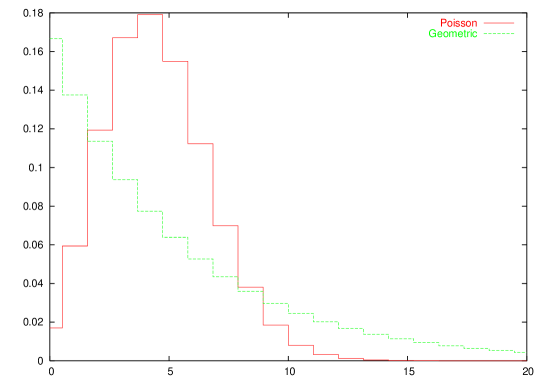
Figure 1: The Poisson and geometric distributions for $\mu=5$.

To counteract the bias in favour of Poisson that is introduced if we just select the best fitting model, we would like to compute the third term of Equation 4, which now characterises the parametric complexity. But as it turns out, both models have an infinite parametric complexity; the integral in the third term of the approximation also diverges! So in this case it is not immediately clear how the bias should be removed. This is the second reason why we chose to study the Poisson and geometric models. In Section 4 we describe a number of methods that have been proposed in the literature as ways to deal with infinite parametric complexity; in Section 5 they are evaluated evaluate empirically.

Reassuringly, all methods we investigate tend to ‘punish’ the Poisson model, and thus compensate for this overfitting phenomenon. However, the amount by which the Poisson model is punished depends on the method used, so that different methods give different results.

We parameterise both the Poisson and the Geometric family of distributions by the mean $\mu\in(0,\infty)$, to allow for easy comparison. This is possible because for both models, the empirical mean (average) of the observed data is a sufficient statistic. For Poisson, parameterisation by the mean is standard. For geometric, the reparameterisation can be arrived at by noting that in the standard parameterisation, $P(x\mid\theta)=(1-\theta)^{x}\theta$, the mean is given by $\mu=(1-\theta)/\theta$. As a notational reminder the parameter is called $\mu$ henceforth. Conveniently, the ML estimator $\hat{\mu}$ for both distributions is the average of the data (the proof is immediate if we set the derivative to zero).

We will add a subscript p or g to indicate that codelengths are computed with respect to the Poisson model or the geometric model, respectively:

$$L_{\textnormal{\tiny P}}\!\left(x^{n}\mid\mu\right) = -\ln\prod_{i=1}^{n}{e^{-\mu}\mu^{x_{i}}\over x_{i}!}=\sum_{i=1}^{n}\ln(x_{i}!)+n\mu-\ln\mu\sum_{i=1}^{n}x_{i}$$ (5)

$$L_{\textnormal{\tiny G}}\!\left(x^{n}\mid\mu\right) = -\ln\prod_{i=1}^{n}{\mu^{x_{i}}\over(\mu\!+\!1)^{x_{i}+1}}=n\ln(\mu\!+\!1)-\ln\left({\mu\over\mu\!+\!1}\right)\sum_{i=1}^{n}x_{i}$$ (6)

4 Four ways to deal with infinite parametric complexity

In this section we discuss four general ways to deal with the infinite parametric complexity of the Poisson and geometric models when the goal is to do model selection. Each of these four leads to one or sometimes more concrete selection criteria which we put into practice and evaluate in Section 5.

4.1 BIC/ML

One way to deal with the diverging term of the approximation is to just ignore it. The model selection criterion that results corresponds to only a very rough approximation of any real universal code, but it has been used and studied extensively. It was proposed both by Rissanen [15] and Schwarz [21] in 1978. Schwarz derived it as an approximation to the Bayesian marginal likelihood, and for this reason, it is best known as the BIC (Bayesian Information Criterion). Rissanen already abandoned the idea in the mid 1980’s in favour of more sophisticated approximations of the NML codelength.

$$L_{\textnormal{\tiny BIC}}\!\left(x^{n}\right)=L\!\left(x^{n}\mid\hat{\mu}\right)+{k\over 2}\ln n$$

Comparing the BIC to the approximated NML codelength we find that in addition to the diverging term, a ${k\over 2}\ln{1\over 2\pi}$ term has also been dropped. This curious difference can be safely ignored in our setup, where $k$ is equal to one for both models so the whole term cancels anyway. According to BIC, we must select the geometric model iff:

$$0<L_{\textnormal{\tiny P,BIC}}\!\left(x^{n}\right)-L_{\textnormal{\tiny G,BIC}}\!\left(x^{n}\right)=L_{\textnormal{\tiny P}}\!\left(x^{n}\mid\hat{\mu}\right)-L_{\textnormal{\tiny G}}\!\left(x^{n}\mid\hat{\mu}\right)$$

We are left with a generalised likelihood ratio test (GLRT). Such a test has the form ${P_{\textnormal{\tiny P}}\!\left(x^{n}\mid\hat{\theta}\right)\over P_{\textnormal{\tiny G}}\!\left(x^{n}\mid\hat{\theta}\right)}{>\atop<}\eta$; the BIC criterion thus reduces to a GLRT with $\eta=0$, which is also known as maximum likelihood (ML) testing. It should be expected that this leads to overfitting and therefore to a bias in favour of the ‘more complex’ Poisson model.

4.2 Restricted ANML

One often used method of rescuing the NML approach to MDL model selection is to restrict the range of values that the parameters can take to ensure that the third term of Equation 4 stays finite.

To compute the approximated parametric complexity of the restricted models we need to establish the Fisher information first. Using the formula $I(\theta)=-E_{\theta}[{d^{2}\over d\theta^{2}}L\!\left(x\mid\theta\right)]$, we get:

$$I_{\textnormal{\tiny P}}\!\left(\mu\right) = -E_{\mu}\left[-{x\over\mu^{2}}\right]={1\over\mu}$$ (7)

$$I_{\textnormal{\tiny G}}\!\left(\mu\right) = -E_{\mu}\left[-{x\over\mu^{2}}+{x+1\over(\mu+1)^{2}}\right]={1\over\mu(\mu+1)}$$ (8)

Now we can compute the last term in the parametric complexity approximation (4):

$$\ln\int_{0}^{\mu^{*}}\kern-11.38092pt\sqrt{I_{\textnormal{\tiny P}}\!\left(\mu\right)}d\mu = \ln\int_{0}^{\mu^{*}}\kern-11.38092pt\mu^{-{1\over 2}}d\mu=\ln\left(2\sqrt{\mu^{*}}\right)$$ (9)

$$\ln\int_{0}^{\mu^{*}}\kern-11.38092pt\sqrt{I_{\textnormal{\tiny G}}\!\left(\mu\right)}d\mu = \ln\int_{0}^{\mu^{*}}\kern-11.38092pt{1\over\sqrt{\mu(\mu+1)}}d\mu=\ln 2\ln\left(\sqrt{\mu^{*}}+\sqrt{{\mu^{*}}+1}\right)$$ (10)

The parametric complexities of the restricted models with parameter ranges $(0,{\mu^{*}})$ are both monotonically increasing functions of ${\mu^{*}}$. However, the parametric complexity of the restricted Poisson model grows faster with ${\mu^{*}}$ than the parametric complexity of the geometric model, indicating that the Poisson model has more descriptive power, even though the models have the same number of parameters. Let the function $\delta({\mu^{*}})$ measure the difference between the parametric complexities. Interestingly, this function is still monotonically increasing in ${\mu^{*}}$ (this is proven in Appendix A). It is also easy to prove that it grows unboundedly in ${\mu^{*}}$.

4.2.1 Basic restricted ANML

We have experimented with restricted models where the parameter range was restricted to $(0,{\mu^{*}})$ for ${\mu^{*}}\in\{10,100,1000\}$.

This means that we obtain a model selection criterion that selects the geometric model iff $0<L_{\textnormal{\tiny P,ANML$({\mu^{*}})$}}\!\left(x^{n}\right)-L_{\textnormal{\tiny G,ANML$({\mu^{*}})$}}\!\left(x^{n}\right)=L_{\textnormal{\tiny P}}\!\left(x^{n}\mid\hat{\mu}\right)-L_{\textnormal{\tiny G}}\!\left(x^{n}\mid\hat{\mu}\right)+\delta({\mu^{*}})$. This is equivalent to a GLRT with threshold $\delta({\mu^{*}})$. For $\lim{\mu^{*}}\downarrow 0$ we obtain the BIC/ML selection criterion; higher values of ${\mu^{*}}$ translate to a selection threshold more in favour of the geometric model.

An obvious conceptual problem with the resulting code is that the imposed restriction is quite arbitrary and requires a priori knowledge about the generating process. But the parameter range can be interpreted as a hyper-parameter, which can be incorporated into the code using several techniques, some of which we will discuss.

4.2.2 Two-part ANML

The most obvious way to generalise the restricted ANML codelength is to separately encode a parameter range using some suitable discretisation. For a sequence with empirical mean $\hat{\mu}$, we encode the integer $b=\left\lceil\log_{2}\hat{\mu}\right\rceil$. After outputting $b$ the code length for the rest of the data is computed using restricted ANML with range $(2^{b-1},2^{b}]$. By taking the logarithm we ensure that the number of bits used in coding the parameter range grows at a negligible rate compared to the code length of the data itself, but we admit that the code for the parameter range admits of much greater sophistication. We do not really have reason to assume that the optimal discretisation should be the same for the Poisson and geometric models for example.

The two-part code is slightly redundant, since code words are assigned to data sequences of which the ML estimator lies outside the range that was encoded in the first part – such data sequences cannot occur, since for such a sequence we would have encoded a different range. Furthermore, the two-part code is no longer minimax optimal, so it is no longer clear why it should be better than other universal codes which are not minimax optimal. However, as argued in [11], whenever the minimax optimal code is not defined, we should aim for a code $L$ which is ‘close’ to minimax optimal in the sense that, for any compact subset ${\cal M}^{\prime}$ of the parameter space, the additional regret of $L$ on top of the NML code for ${\cal M}^{\prime}$ should be small, e.g. $O(\log\log n)$. The two-part ANML code is one of many universal codes satisfying this ‘almost minimax optimality’. While it may not be better than another almost minimax optimal universal code, it certainly is better than universal codes which do not have the almost minimax optimality property.

4.2.3 Renormalised Maximum Likelihood

Related to the two-part restricted ANML, but more elegant, is Rissanen’s renormalised maximum likelihood (RNML) code, [19, 11]. This is perhaps the most widely known approach to deal with infinite parametric complexity. The idea here is, rather than explicitly encoding a parameter range in which we know the ML estimator to lie, to treat the range $(0,{\mu^{*}})$ as a hyper-parameter. The probability of a sequence is computed using the maximum likelihood value for the hyper-parameter, but just as ordinary NML has to be normalised, the probability distribution thus obtained must be renormalised to ensure that it sums to $1$.

If this still leads to infinite parametric complexity, we define a hyper-hyper-parameter. We repeat the procedure until the resulting complexity is finite. Unfortunately, in our case, after the first renormalisation, both parametric complexities are still infinite; we did not manage to perform a second renormalisation. Therefore, we have not experimented with the RNML code.

4.3 Plug-in predictive code

The plug-in predictive code, or prequential ML code, is an attractive universal code because it is usually a lot easier to implement than either NML or a Bayesian code. Moreover, its implementation hardly requires any arbitrary decisions. Here the outcomes are coded sequentially using the probability distribution indexed by the ML estimator for the previous outcomes [8, 16]; for a general introduction see [11].

$$L_{\textnormal{\tiny PIPC}}\!\left(x^{n}\right)=\sum_{i=1}^{n}L\!\left(x_{i}\mid\hat{\mu}(x^{i-1})\right)$$

where $L\!\left(x_{i}\mid\hat{\mu}(x^{i-1})\right)=-\ln P\!\left(x_{i}\mid{\hat{\mu}(x^{i-1})}\right)$ is the number of nats needed to encode outcome $x_{i}$ using the code based on the ML estimator on $x^{i-1}$. We further discuss the motivation for this code in Section 5.1.2.

For both the Poisson model and the geometric model, the maximum likelihood estimator is not well-defined until after a nonzero outcome has been observed (since $0$ is not inside the allowed parameter range). This means that we need to use another code for the first few outcomes. It is not really clear how we can use the model assumption (Poisson or geometric) here, so we pick a simple code for the nonnegative integers that does not depend on the model. This will result in the same codelength for both models; therefore it does not influence which model is selected. Since there are usually only very few initial zero outcomes, we may reasonably hope that the results are not too distorted by our way of handling this startup problem. We note that this startup problem is an inherent feature of the predictive plug-in approach [8, 17], and our way of handling it is in line with the suggestions in [8].

4.4 Objective Bayesian approach

In the Bayesian framework we select a prior $w(\theta)$ on the unknown parameter and compute the marginal likelihood $P_{\textnormal{\tiny BAYES}}\!\left(x^{n}\right)=\int_{\Theta}P\!\left(x^{n}\mid\theta\right)w(\theta)d\theta$, which corresponds to a universal code $L_{\textnormal{\tiny BAYES}}\!\left(x^{n}\right)=-\ln P_{\textnormal{\tiny BAYES}}\!\left(x^{n}\right)$. Like the NML, this can be approximated with an asymptotic formula. For exponential families such as the models under consideration, we have [1]:

$$L_{\textnormal{\tiny ABAYES}}\!\left(x^{n}\right):=L\!\left(x^{n}\mid\hat{\theta}\right)+{k\over 2}\ln{n\over 2\pi}+\ln{\sqrt{\det I(\theta)}\over w(\theta)},$$ (11)

where $L_{\textnormal{\tiny ABAYES}}\!\left(x^{n}\right)-L_{\textnormal{\tiny BAYES}}\!\left(x^{n}\right)\rightarrow 0$ as $n\rightarrow\infty$. Objective Bayesian reasoning suggests we use Jeffreys’ prior [4] for several reasons; one reason is that it is uniform over all ‘distinguishable’ elements of the model, which implies that the obtained results are independent of the parametrisation of the model [1]. It is defined as follows:

$$w(\theta)={\sqrt{\det I(\theta)}\over\int_{\Theta}\sqrt{\det I(\theta)}d\theta}$$ (12)

Unfortunately, the normalisation factor in Jeffreys’ prior diverges for both the Poisson model and the geometric model. But if one is willing to accept a so-called improper prior, which is not normalised, then it is possible to compute a perfectly proper Bayesian posterior, after observing the first outcome, and use that as a prior to compute the marginal likelihood of the rest of the data. The resulting universal codes with lengths $L_{\textnormal{\tiny BAYES}}\!\left(x_{2},\ldots,x_{n}\mid x_{1}\right)$ are, in fact, conditional on the first outcome. Recent work by Li and Barron [14] suggests that, at least asymptotically and for one-parameter models, the universal code achieving the minimal expected redundancy conditioned on the first outcome is given by the Bayesian universal code with the improper Jeffreys’ prior. Li and Barron only prove this for scale and location models, but their result at least suggests that the same would still hold for general exponential families such as Poisson and geometric. It is possible to define MDL inference in terms of either the expected redundancy or of the worst-case regret. In fact, the resulting procedures are very similar, see [2]. Thus, we have a tentative justification for using Jeffreys’ prior also from an MDL point of view, on top of its justification in terms of objective Bayes.

To make this idea more concrete, we compute Jeffreys’ posterior after observing one outcome, and use it to find the Bayesian marginal likelihoods. We write $x_{i}^{j}$ to denote $x_{i},\ldots,x_{j}$ and $\hat{\mu}(x_{i}^{j})$ to indicate which outcomes determine the ML estimator, finally we abbreviate $s_{n}=x_{1}+\ldots+x_{n}$. The goal is to compute $P_{\textnormal{\tiny BAYES}}\!\left(x_{2}^{n}\mid x_{1}\right)$ for the Poisson and geometric models. As before, the difference between the corresponding codelengths defines a model selection criterion. We also compute $P_{\textnormal{\tiny ABAYES}}\!\left(x_{2}^{n}\mid x_{1}\right)$ for both models, the approximated version of the same quantity, based on approximation formula (11). Equations for the Poisson and geometric models are presented below.

Bayesian code for the Poisson model

We compute Jeffreys’ improper prior and the posterior after observing one outcome:

$$w_{\textnormal{\tiny P}}\!\left(\mu\right) \propto \sqrt{I_{\textnormal{\tiny P}}\!\left(\mu\right)}=\mu^{-{1\over 2}}$$ (13)

$$w_{\textnormal{\tiny P}}\!\left(\mu\mid x_{1}\right) = {P_{\textnormal{\tiny P}}\!\left(x_{1}\mid\mu\right)w_{\textnormal{\tiny P}}\!\left(\mu\right)\over\int_{0}^{\infty}P_{\textnormal{\tiny P}}\!\left(x_{1}\mid\theta\right)w_{\textnormal{\tiny P}}\!\left(\theta\right)d\theta}={e^{-\mu}\mu^{x_{1}-{1\over 2}}\over\Gamma(x_{1}+{1\over 2})}$$ (14)

From this we can derive the marginal likelihood of the rest of the data. The details of the computation are omitted for brevity.

$$P_{\textnormal{\tiny P,BAYES}}\!\left(x_{2}^{n}\mid x_{1}\right) = \int_{0}^{\infty}\kern-8.5359ptP_{\textnormal{\tiny P}}\!\left(x_{2}^{n}\mid\mu\right)w_{\textnormal{\tiny P}}\!\left(\mu\mid x_{1}\right)d\mu$$ (15)

$$= {\Gamma(s_{n}+{1\over 2})\over\Gamma(x_{1}+{1\over 2})}/\left(n^{s+{1\over 2}}\prod_{i=2}^{n}x_{i}!\right)$$

We also compute the approximation for the Poisson model using (11):

$$L_{\textnormal{\tiny P,ABAYES}}\!\left(x_{2}^{n}\mid x_{1}\right)=L_{\textnormal{\tiny P}}\!\left(x_{2}^{n}\mid\hat{\mu}(x_{2}^{n}\right))+\hbox{${1\over 2}$}\ln{n\over 2\pi}+\ln{\sqrt{I_{\textnormal{\tiny P}}\!\left(\hat{\mu}(x_{2}^{n}\right))}\over w_{\textnormal{\tiny P}}\!\left(\hat{\mu}(x_{2}^{n}\right)\mid x_{1})}\\ =L_{\textnormal{\tiny P}}\!\left(x_{2}^{n}\mid\hat{\mu}(x_{2}^{n}\right))+\hbox{${1\over 2}$}\ln{n\over 2\pi}+\hat{\mu}(x_{2}^{n})-x_{1}\ln\hat{\mu}(x_{2}^{n})+\ln\Gamma(x_{1}+\hbox{${1\over 2}$})$$ (16)

Bayesian code for the geometric model

We perform the same computations for the geometric model. Jeffreys’ improper prior and its posterior after one outcome are:

$$w_{\textnormal{\tiny G}}\!\left(\mu\right) \propto \mu^{-{1\over 2}}(\mu+1)^{-{1\over 2}}$$ (17)

$$w_{\textnormal{\tiny G}}\!\left(\mu\mid x_{1}\right) = (x_{1}+\hbox{${1\over 2}$})\mu^{x_{1}-{1\over 2}}(\mu+1)^{-x_{1}-{3\over 2}}$$ (18)

$$P_{\textnormal{\tiny G,BAYES}}\!\left(x^{n}\right) = (x_{1}+\hbox{${1\over 2}$}){\Gamma(s+{1\over 2})\Gamma(n)\over\Gamma(n+s+{1\over 2})}$$ (19)

For the approximation we obtain:

$$L_{\textnormal{\tiny G,ABAYES}}\!\left(x_{2}^{n}\mid x_{1}\right)=L_{\textnormal{\tiny G}}\!\left(x_{2}^{n}\mid\hat{\mu}(x_{2}^{n}\right))+{1\over 2}\ln{n\over 2\pi}+\\ x_{1}\ln\left(1+{1\over\hat{\mu}(x_{2}^{n})}\right)+\hbox{${1\over 2}$}\ln(\hat{\mu}(x_{2}^{n}))-\ln(x_{1}+\hbox{${1\over 2}$})$$ (20)

5 Results

We have now described how to compute or approximate the length of a number of different universal codes, which can be used in an MDL model selection framework. The MDL principle tells us to select the model using which we can achieve the shortest codelength for the data. This coincides with the Bayesian maximum a-posteriori (MAP) model with a uniform prior on the models. In this way each method for computing or approximating universal codelengths defines a model selection criterion, which we want to compare empirically.

In addition to the criteria that are based on universal codes, as developed in Section 4, we define one additional, ‘ideal’ criterion to serve as a reference by which the others can be evaluated. The known $\mu$ criterion cheats a little bit: it computes the code length for the data with knowledge of the mean of the generating distribution. If the mean is $\mu$, then the known $\mu$ criterion selects the Poisson model if $L_{\textnormal{\tiny P}}\!\left(x^{n}\mid\mu\right)<L_{\textnormal{\tiny G}}\!\left(x^{n}\mid\mu\right)$. Since this criterion uses extra knowledge about the data, it should be expected to perform better than the other criteria.

We perform two types of test on the selection criteria:

• Error probability measurements. Here we select a mean and a generating distribution (Poisson or geometric), then artificially generate samples with that mean of varying size. We offset the sample size to the observed probabilities of error of the selection criteria. This test can be generalised by putting a prior on the generating distribution, such that a fixed percentage of samples is generated using a geometric distribution, and the remainder using Poisson.

• Calibration testing. In the Bayesian framework the criteria do not only output which model is most likely (the MAP model), but each model is also assigned a probability. This can also be understood from an MDL perspective via the correspondence between code lengths and probabilities we mentioned earlier. If a well calibrated selection criterion assigns a probability $p$ to the data being Poisson distributed, and the criterion is used repeatedly on independently generated data sets, then the frequency with which it actually is Poisson should be close to $p$. To test this we discretise the probability that each criterion assigns to the data being Poisson into a number of ‘bins’. Then we plot for each bin the fraction of samples that actually were Poisson.

Roughly, the results of both tests can be summarized as follows:

• As was to be be expected, the known $\mu$ criterion performs excellently on both tests.

• The criteria based on the plug-in predictive code and BIC/ML exhibit the worst performance.

• The basic restricted ANML criterion yields results that range from good to very bad, depending on the chosen parameter range. Since the range must be chosen without any additional knowledge of the properties of the data, this criterion is a bit arbitrary.

• The results for the two-part restricted ANML and Objective Bayesian criteria are reasonable in all tests we performed; these criteria thus display robustness.

In subsequent sections we will treat the results in more detail. In Section 5.1 we discuss the results of the error probability tests, the calibration test results are presented in Section 5.2.

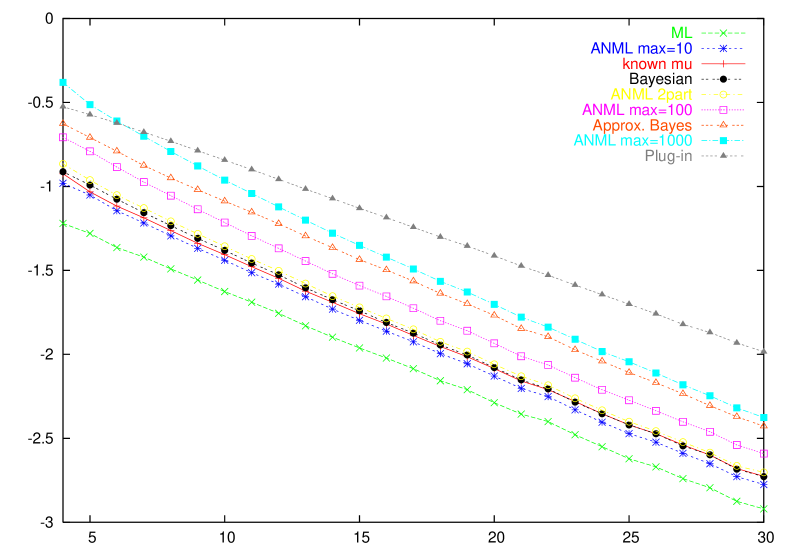
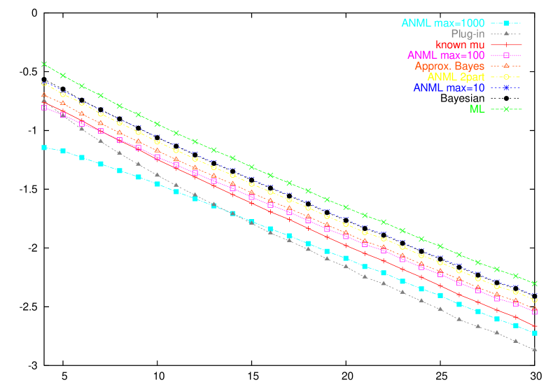
Figure 2: The $\log_{10}$ of the frequency of wrong classification when the data were generated with mean $4$ by the Poisson (top) or geometric (bottom) distributions.

5.1 Error probability

In this section we investigate the probability of error of the model selection criteria through various experiments. We investigate the error probability in more than one way. First we just look at its magnitude – the lower the error probability of a criterion, the better, obviously. However the error probability in itself is only defined given a prior on the generating distribution, because the error probability may differ, depending on whether the data are Poisson or geometrically distributed. Figures 2, 4, 5 and 6 show results of this kind, using different means and different priors on the generating distribution.

The other interesting aspect of error probability is the notion of bias: some criteria are much more likely to misclassify Poisson data than geometric data, or vice versa. By bias we mean the difference between the logs of the error probability for the Poisson and geometric data. This is not the standard statistical definition (which is defined with respect to an estimator), but it is a convenient quantification of our intuitive notion of bias in this setting. A small bias is an important feature of a good model selection criterion. Figure 3 shows the bias of the selection criteria; the top graph simply measures the distance between corresponding lines in the top and bottom graphs of Figure 2. It is important to realize that a criterion may be terribly biased and yet have a very low probability of either type of error – this is why it is necessary to study both aspects. We will say more about bias in our discussion of the individual selection criteria.

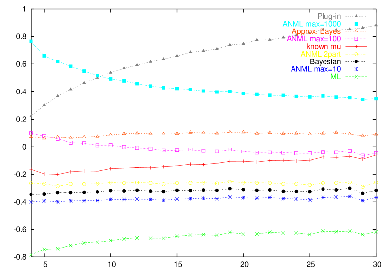
Figure 3: The classification bias (using log base $10$) when the data were generated with mean $4$ (top graph) and mean $16$ (bottom graph).

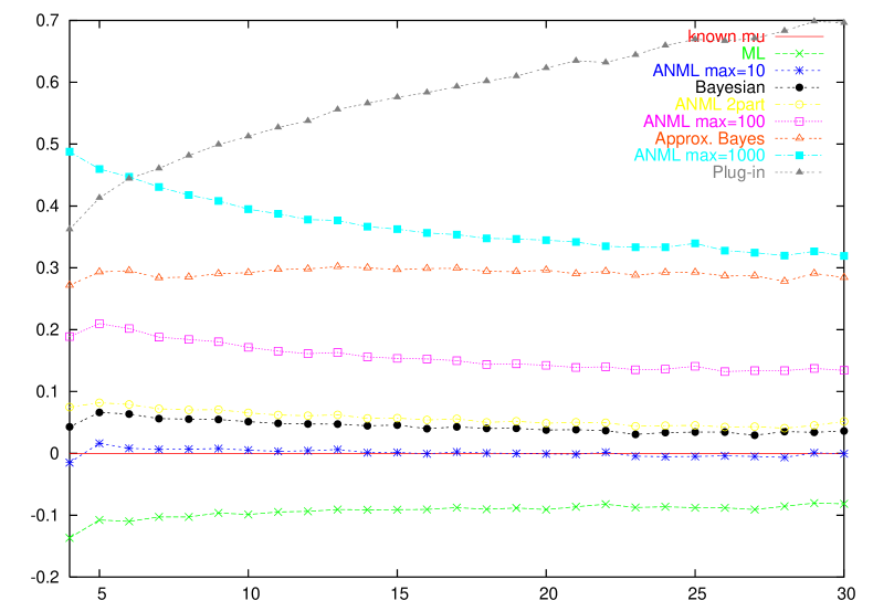
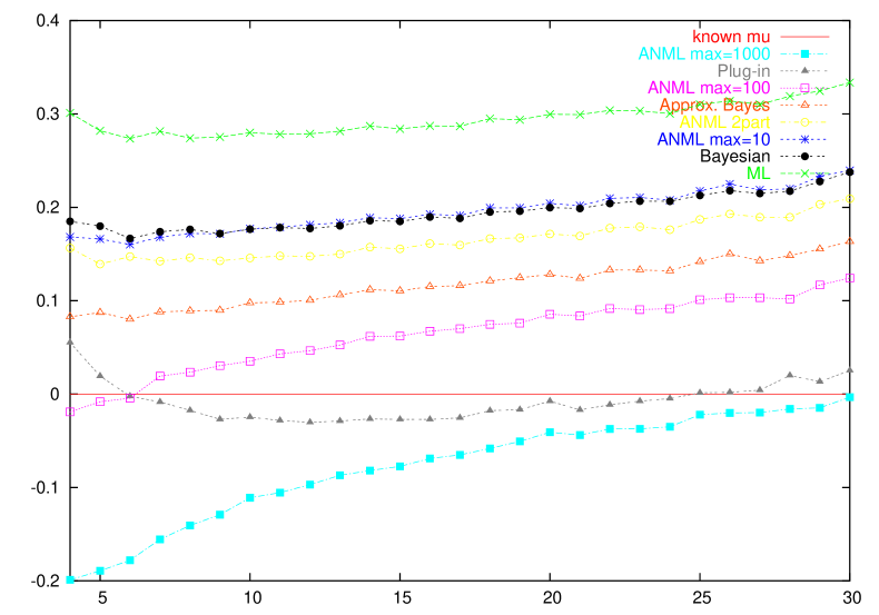
Figure 4: The difference in the $\log_{10}$ of the frequency of wrong classification between each criterion and the known $\mu$ criterion. In the top graph $90\%$ of the data were generated by Poisson, in the bottom graph $10\%$. The mean is $4$.

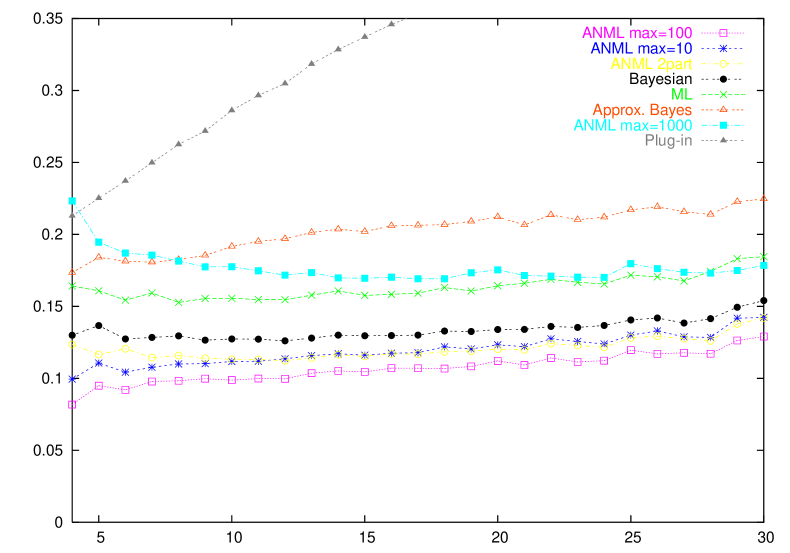
Figure 5: The difference in the $\log_{10}$ of the frequency of wrong classification between each criterion and the known $\mu$ criterion. Half the data were generated by the Poisson distribution, and half by the geometric distribution. The mean is $4$.

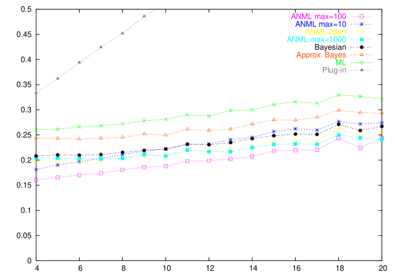
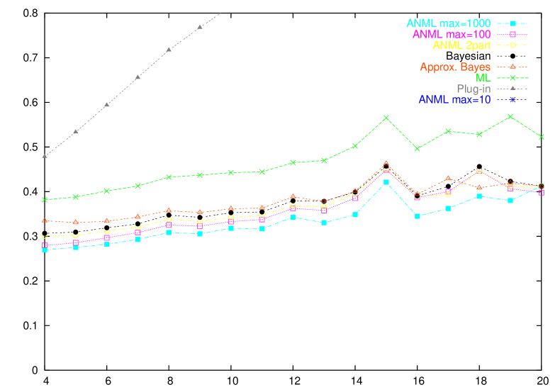
Figure 6: The difference in the $\log_{10}$ of the frequency of wrong classification between each criterion and the known $\mu$ criterion. Half the data were generated by the Poisson distribution, and half by the geometric distribution. The mean is $8$ in the top graph and $16$ in the bottom graph.

5.1.1 Known $\mu$

The theoretical analysis of the known $\mu$ criterion is helped by the circumstance that (1) one of the two hypotheses equals the generating distribution and (2) the sample consists of outcomes which are i.i.d. according to this distribution. Cover and Thomas [7] use Sanov’s Theorem to show that in such a situation, the probability of error decreases exponentially in the sample size. If the Bayesian MAP model selection criterion is used then the following happens: if the data are generated using $\textnormal{Poisson}[\mu]$ then the probability of error decreases exponentially in the sample size, with some error exponent; if the data are generated with $\textnormal{Geom}[\mu]$ then the overall probability is exponentially decreasing with the same exponent [7, Theorem 12.9.1 on page 312 and text thereafter]. Thus, we expect that the line for the “known $\mu$” criterion in Figure 2 is straight on a logarithmic scale, with a slope that is equal on the top and bottom graphs. This proves to be the case.

In Figures 4, 5 and 6 the log of the error frequency of the known $\mu$ criterion is subtracted from the logs of the error frequencies of the other criteria. This brings out the differences in performance in more detail. The known $\mu$ criterion, which is perfectly calibrated (as we will observe later) and which also has a low probability of error under all circumstances (although biased criteria can sometimes do better if the bias is in the right direction), is thus treated as a baseline of sorts.

5.1.2 Poor performance of the plug-in criterion

One feature of Figure 2 that immediately attracts attention is the unusual slope of the error rate line of the plug-in criterion, which clearly favours the geometric distribution. We did not obtain completely unbiased results in any of our experiments, but only the bias of the plug-in criterion grows substantially as the sample size increases. Figure 3 shows how at $n=30$ its bias in favour of the geometric model reaches a level where a sample is about $10^{0.88}\approx 7$ times more likely to be misclassified as geometric than as Poisson.

While this behaviour may seem appropriate if the data are judged more likely to come from a geometric distribution, there is actually a strong argument that even under those circumstances it is not. As pointed out in the beginning of this section, beside the bias also the magnitude of the error probability should be taken into account. Suppose that we put a fixed prior on the generating distribution, with nonzero probability for both distributions. The marginal probability of error is a linear combination of the probabilities of error for the two generating distributions; as such it is dominated by the probability of error with the worst exponent. So if minimising the probability of error is our goal, then we must conclude that the behaviour of the plug-in criterion is suboptimal. (On a side note, minimising the probability of error with respect to a fixed prior is not the goal of classical hypothesis testing, since in that setting the two hypotheses do not play a symmetrical role.) To illustrate, the bottom graph in Figure 4 shows that, even if there is only a $10\%$ chance that the data are Poisson, then the plug-in criterion still has a worse (marginal) probability of error than “known $\mu$” as soon as the sample size reaches 25. Figure 5 shows what happens if the prior on the generating distribution is uniform – using the plug-in criterion immediately yields the largest probability of error of all the criteria under consideration. This effect only becomes stronger if the mean is higher.

This strangely poor behaviour of the plug-in criterion initially came as a complete surprise to us. Theoretical literature certainly had not suggested it. Rather the contrary: in 1989 Rissanen writes that “it is only because of a certain inherent singularity in the process [of plug-in coding], as well as the somewhat restrictive requirement that the data must be ordered, that we do not consider the resulting predictive code length to provide another competing definition for the stochastic complexity, but rather regard it as an approximation.” [17] There are also many results showing that the regret for the plug-in code grows as ${k\over 2}\ln n$, the same as the regret for the NML code, for a variety of models. Examples are [20, 9, 22]. So we were extremely puzzled by these results at first.

To gain intuition as to why the plug-in code should behave so strangely, note that the variance of a geometric distribution is much larger than the variance of the Poisson distribution with the same mean. This suggests that the penalty for using $\hat{\mu}$ rather than $\mu$ to code each consecutive outcome is higher for the Poisson model. The accumulated difference accounts for the difference in regret.

We have made this intuition precise in a separate publication. In [10] we prove that for single parameter exponential families, the regret for the plug-in code grows with ${1\over 2}\ln(n)\textnormal{Var}_{P}(X)/\textnormal{Var}_{M}(X)$, where $n$ is the sample size, $P$ is the generating distribution and $M$ is the best element of the model (the element of $\mathcal{M}$ for which $D(P\parallel M)$ is minimised). The plug-in model has the same regret (to $O(1)$) as the NML model if and only if the variance of the generating distribution is the same as the variance of the best element of the model. The existing literature studies the case where $M=P$, so automatically $\textnormal{Var}_{M}(X)=\textnormal{Var}_{P}(X)$.

5.1.3 ML/BIC

Beside known $\mu$ and plug-in, all criteria seem to share more or less the same error exponent. Nevertheless, they still show differences in bias. While we have to be careful to avoid over-interpreting our results, we find that the ML criterion consistently displays the largest bias in favour of the Poisson model. Figure 3 shows how the ML criterion misclassifies a sequence as Poisson about four times more often than the other way around when the mean is $4$; when the mean is raised to $16$ bias has increased even further, to a ratio of twenty to one.

This illustrates how the Poisson model appears to have a greater descriptive power, even though the two models have the same number of parameters, an observation which we hinted at in Section 3. Intuitively, the Poisson model allows more information about the data to be stored in the parameter estimate. All the other selection criteria compensate for this effect, by giving a higher probability to the geometric model. (In terms of coding, the Poisson codelength is increased by more than the geometric codelength.) Comparing the two graphs in Figure 3, we find that as the mean of the generating distribution is increased, the prediction errors for all criteria except ML move closer together, showing that for higher means it becomes even more worthwhile to try and compensate for the favouritism of ML/BIC.

5.1.4 Basic restricted ANML

We have seen that the ML/BIC criterion shows the largest bias for the Poisson model. The top graph of Figure 3 shows that the largest bias in the other direction is achieved by ANML ${\mu^{*}}=1000$ (until the sample gets so large that, inevitably, it is overtaken by the plug-in criterion). Apparently the ANML criterion overcompensates. In a way it is obvious that we could obtain such a result since we observed in Section 4.2 that ANML leads to a selection criterion that is equivalent to a GLRT with a selection threshold that is an unbounded, monotonically increasing function of ${\mu^{*}}$. Essentially, by choosing an appropriate ${\mu^{*}}$ we can get any bias in favour of the geometric model. We conclude that it does not really make sense to use an arbitrarily chosen restricted parameter domain to repair the NML model when it is undefined.

5.1.5 Objective Bayes and two-part restricted ANML

We will not try to interpret the differences in error probability for the (approximated) Bayesian and ANML 2-part criteria. Since we are using different selection criteria we should expect at least some differences in the results. These differences are exaggerated by our setup with its low mean and small sample size.

Figures 4–6 show that the probability of error for these criteria tends to decrease at a slightly lower rate than for known $\mu$ (except when the prior on the generating distribution is heavily in favour of Poisson). While we do not understand this phenomenon well enough so as to prove it mathematically, it is of course consistent with the general rule that with more prior uncertainty, more data are needed to make the right decision. It may be that all the information contained within a sample can be used to improve the resolution of the known $\mu$ criterion, while for the other criteria some of that information has to be sacrificed in order to estimate the parameter value.

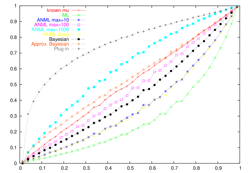
Figure 7: Calibration: probability that the model assigned to the data being Poisson against the frequency with which it actually was Poisson. The sample size is $8$ and the mean is $8$.

5.2 Calibration

The classical interpretation of probability is frequentist: an event has probability $p$ if in a repeated experiment the frequency of the event converges to $p$. This interpretation is no longer really possible in a Bayesian framework, since prior assumptions often cannot be tested in a repeated experiment. For this reason, calibration testing is avoided by some Bayesians who may put forward that it is a meaningless procedure from a Bayesian perspective. On the other hand, we take the position that even with a Bayesian hat on, one would like one’s inference procedure to be calibrated – in the idealised case in which identical experiments are performed repeatedly, probabilities should converge to frequencies. If they do not behave as we would expect even in this idealised situation, then how can we trust inferences based on such probabilities in the real world with all its imperfections? We feel that calibration testing is too important to ignore, safeguarding against inferences or predictions that bear little relationship to the real world. Moreover, in the so-called “objective Bayes” branch of Bayesian statistics, one does emphasise Bayesian procedures with good frequentist behaviour.[3] At least in restricted contexts [6, 5], Jeffreys’ prior has the property that the Kullback-Leibler divergence between the true distribution and the posterior converges to zero quickly, no matter what the true distribution is. Consequently, after observing only a limited number of outcomes, it should already be possible to interpret the posterior as an almost “classical” distribution in the sense that it can be verified by frequentist experiments [6].

In the introduction we have indicated the correspondence between codelengths and probability. If the universal codelengths for the different criteria correspond to probabilities that make sense in a frequentist way, then the Bayesian a posteriori probabilities of the two models should too. To test this, we generate a sample and compute the a posteriori probability that it is generated by the Poisson model, for each of the selection criteria. This probability is discretised into 40 bins. For each bin we count the number of sequences that actually were generated by Poisson. If the a posteriori Bayesian probability that the model is Poisson makes any sense in a frequentist way, then the result should be a more or less straight diagonal.

We use mean $8$ and sample size $8$ because on the one hand we want a large enough sample size that the posterior has converged to something reasonable, but on the other hand if we choose the sample size even larger it becomes exceedingly unlikely that a sequence is generated of which the probability that it is Poisson is estimated near $0.5$, so we would need to generate an infeasibly large number of samples to get accurate results.

Our results are in Figure 7. The “known $\mu$” criterion is clearly perfectly calibrated, which makes sense since its implicit prior distribution on the mean of the generating distribution puts all probability on the actual mean, so the prior perfectly reflects the truth in this case. Under such circumstances Bayesian and frequentist probability become the same, so we get a perfect answer.

Clearly the ML and plug-in criteria, which were observed to be the most biased in Section 5.1, are again the two worst performers. When the probability that the data is Poisson distributed is assessed by the ML criterion to be around $0.5$, the real frequency of the data being Poisson distributed is only about $0.2$. The plug-in criterion behaves even worse, assigning a probability of $0.6$ to the Poisson model for sequences of which only $0.2$ actually were Poisson distributed. The other criteria are better calibrated.

The calibration test does seem to be very sensitive, exposing weaknesses of selection criteria much more clearly than error rate tests. In fact, if circumstances allow it, one of the best ways to engineer a selection criterion may be to just use the GLRT, optimising the threshold for performance on a calibration test.

6 Summary and conclusion

We have performed error rate tests and calibration tests to study the properties of a number of model selection criteria. These criteria are based on the MDL philosophy and involve computing the code length of the data with the help of the model. There are several ways to compute such a code, but the preferred method, the Normalised Maximum Likelihood (NML) code, cannot be applied since it is not well-defined for the Poisson and geometric models that we consider.

We have experimented with the following alternative ways of working around this problem: (1) using BIC which is a simplification of approximated NML (ANML), (2) ANML with a restricted parameter range, this range being either fixed or encoded separately, (3) a Bayesian model using Jeffreys’ prior, which is improper for the case at hand but which can be made proper by conditioning on the first outcome of the sample, and (4) a plug-in code which always codes the new outcome using the distribution indexed by the maximum likelihood estimator for the preceding outcomes.

Both BIC and ANML with a fixed restricted parameter range define a GLRT test and can be interpreted as methods to choose an appropriate threshold. BIC implies a neutral threshold, so the criterion will become biased in favour of the model which is most susceptible to overfitting. We found that even though both models under consideration have only one parameter, a GLRT with neutral threshold tends to be biased in favour of Poisson. ANML implies a threshold that counteracts this bias, but for every such threshold value there exists a corresponding parameter range, so it doesn’t provide any more specific guidance in selecting that threshold. If the parameter range is separately encoded, this problem is avoided and the resulting criterion behaves competitively, although it is not calibrated as well as the Bayesian criterion and the two-part codelength is slightly redundant.

The Bayesian criterion displays reasonable performance both on the error rate experiments and the calibration test. The Bayesian universal codes for the models are not redundant and admit an MDL interpretation as minimising worst-case codelength in an expected sense (Section 4.4).

The plug-in criterion has a bias in favour of the geometric model that depends strongly on the sample size. As a consequence its error rate decreases more slowly in the sample size if we put a prior on the generating distribution that assigns nonzero probability to both models. This result was surprising to us and has led to a theoretical analysis of the codelength of the plug-in code in [10]. It turns out that the regret of the plug-in code does not necessarily grow with ${k\over 2}\ln n$ like the NML and Bayesian codes do, if the sample is not distributed according to any element of the model. We conjecture that model selection based on plug-in codes continues to behave suboptimally in more general settings. However, we should note that there are strong limits to ‘how bad things can get’. Various results [2] indicate that model selection based on plug-in codes must eventually select the correct model (if such a model exists), even when the number of models under consideration is unbounded.

In conclusion, while NML certainly seems a sensible approach to defining model selection criteria, when it is undefined it is impossible to minimise the worst case regret. There are many different methods to deal with this problem, some of which work reasonably well and some of which work surprisingly badly. The fundamental question remains: if it is not possible to minimise the worst case regret, then what exactly should we optimise?

Appendix A Proofs

Proposition 1

The parametric complexity of the restricted geometric model subtracted from the parametric complexity of the restricted Poisson model is monotonically increasing.

• We have to show that the derivative is nonnegative everywhere. Consecutive inequalities should be interpreted as having a “follows from” relationship.

  $$0 \leq {d\over dx}\left(\ln\sqrt{x}-\ln\ln(\sqrt{x}+\sqrt{x+1})\right)$$

  $$= {1\over 2x}-{1\over\ln(\sqrt{x}+\sqrt{x+1})}\cdot{1\over 4x+2+4\sqrt{x}\sqrt{x+1}}$$

  $$x \leq \ln(\sqrt{x}+\sqrt{x+1})(2x+1+2\sqrt{x}\sqrt{x+1})$$

  $${x\over 4x+1} \leq \ln(\sqrt{x}+\sqrt{x+1})$$

  $${d\over dx}{x\over 4x+1} \leq {d\over dx}\ln(\sqrt{x}+\sqrt{x+1})$$

  $${1\over(4x+1)^{2}} \leq {1\over 2\sqrt{x}\sqrt{x+1}}$$

  $$16x^{2}+8x+1 \geq 2\sqrt{x}\sqrt{x+1}$$

  From convexity of the logarithm, we have $\ln(x+{1\over 2})\geq{1\over 2}\ln(x)+{1\over 2}\ln(x+1)=\ln(\sqrt{x}\sqrt{x+1})$; by monotonicity of logarithm it follows that $x+{1\over 2}\geq\sqrt{x}\sqrt{x+1}$; we use this to bound the right hand side term in the final inequality. Thus the proof follows from $16x^{2}+8x+1\geq 2x+1$. $\Box$

References

- [1] V. Balasubramanian. Statistical inference, Occam’s Razor, and statistical mechanics on the space of probability distributions. Neural Computation, 9:349–368, 1997.
- [2] A. Barron, J. Rissanen, and B. Yu. The minimum description length principle in coding and modeling. IEEE Transactions on Information Theory, 44(6):2743–2760, 1998. Special Commemorative Issue: Information Theory: 1948-1998.
- [3] Jim Berger. Personal communication, 2004.
- [4] José Bernardo and Adrian F.M. Smith. Bayesian Theory. Wiley, 1994.
- [5] Bernard Clarke and Andrew Barron. Jeffreys’ prior is asymptotically least favourable under entropy risk. The Journal of Statistical Planning and Inference, 41:37–60, 1994.
- [6] Bertrand Clarke and Andrew Barron. Information theoretic asymptotics of bayes methods. IEEE Transactions on Information Theory, 36:453–471, 1990.
- [7] T.M. Cover and J.A. Thomas. Elements of Information Theory. Wiley Interscience, New York, 1991.
- [8] A.P. Dawid. Present position and potential developments: Some personal views, statistical theory, the prequential approach. Journal of the Royal Statistical Society, Series A, 147(2):278–292, 1984.
- [9] L. Gerensce’r. Order estimation of stationary gaussian ARMA processes using Rissanen’s complexity. Technical report, Computer and Automation Institute of the Hungarian Academy of Sciences, 1987.
- [10] P. Grünwald and S. de Rooij. Asymptotic log-loss of prequential maximum likelihood codes. Submitted for publciation, February 2005. Avalaible at the CORR Computer Science arXiv.
- [11] Peter D. Grünwald. MDL tutorial. In Peter D. Grünwald, In Jae Myung, and Mark A. Pitt, editors, Advances in Minimum Description Length: Theory and Applications. MIT Press, 2005.
- [12] Peter D. Grünwald, In Jae Myung, and Mark A. Pitt, editors. Advances in Minimum Description Length: Theory and Applications. MIT Press, 2005.
- [13] Aaron D. Lanterman. Hypothesis testing for Poisson versus geometric distributions using stochastic complexity. In Peter D. Grünwald, In Jae Myung, and Mark A. Pitt, editors, Advances in Minimum Description Length: Theory and Applications. MIT Press, 2005.
- [14] Feng Liang and Andrew Barron. Exact minimax predictive density estimation and MDL. In Peter D. Grünwald, In Jae Myung, and Mark A. Pitt, editors, Advances in Minimum Description Length: Theory and Applications. MIT Press, 2005.
- [15] J. Rissanen. Modeling by the shortest data description. Automatica, 14:465–471, 1978.
- [16] J. Rissanen. Universal coding, information, prediction and estimation. IEEE Transactions on Information Theory, 30:629–636, 1984.
- [17] J. Rissanen. Stochastic Complexity in Statistical Inquiry. World Scientific Publishing Company, 1989.
- [18] J. Rissanen. Fisher information and stochastic complexity. IEEE Transactions on Information Theory, 42(1):40–47, 1996.
- [19] J. Rissanen. MDL denoising. IEEE Transactions on Information Theory, 46(7):2537–2543, 2000.
- [20] Jorma Rissanen. A predictive least squares principle. IMA Journal of Mathematical Control and Information, 3:211–222, 1986.
- [21] G. Schwarz. Estimating the dimension of a model. The Annals of Statistics, 6(2):461–464, 1978.
- [22] C.Z. Wei. On predictive least squares principles. Annals of Statistics, 20(1):1–42, 1990.