A Time-Optimal Delaunay Refinement Algorithm in Two Dimensions

Abstract

We propose a new refinement algorithm to generate size-optimal quality-guaranteed Delaunay triangulations in the plane. The algorithm takes $O(n\log n+m)$ time, where $n$ is the input size and $m$ is the output size. This is the first time-optimal Delaunay refinement algorithm.

1 Introduction

Geometric domain discretizations (i.e., meshing) are essential for computer-based simulations and modeling. It is important to avoid small (and also very large) angles in such discretizations in order to reduce numerical and interpolation errors [SF73]. Delaunay triangulation maximizes the smallest angle among all possible triangulations of a given input and hence is a powerful discretization tool. Depending on the input configuration, however, Delaunay triangulation can have arbitrarily small angles. Thus, Delaunay refinement algorithms which iteratively insert additional points were developed to remedy this problem. There are other domain discretization algorithms including the quadtree-based algorithms [BEG94, MV00] and the advancing front algorithms [Loh96]. Nevertheless, Delaunay refinement method is arguably the most popular due to its theoretical guarantee and performance in practice. Many versions of the Delaunay refinement is suggested in the literature [Che89b, EG01, Mil04, MPW03, Rup93, She97, Üng04].

The first step of a Delaunay refinement algorithm is the construction of a constrained or conforming Delaunay triangulation of the input domain. This initial Delaunay triangulation is likely to have bad elements. Delaunay refinement then iteratively adds new points to the domain to improve the quality of the mesh and to ensure that the mesh conforms to the boundary of the input domain. The points inserted by the Delaunay refinement are Steiner points. A sequential Delaunay refinement algorithm typically adds one new vertex at each iteration. Each new vertex is chosen from a set of candidates — the circumcenters of bad triangles (to improve mesh quality) and the mid-points of input segments (to conform to the domain boundary). Chew [Che89b] showed that Delaunay refinement can be used to produce quality-guaranteed triangulations in two dimensions. Ruppert [Rup93] extended the technique for computing not only quality-guaranteed but also size-optimal triangulations. Later, efficient implementations [She97], extensions to three dimensions [DBS92, She97], generalization of input type [She97, MPW03], and parallelization of the algorithm [STÜ02] were also studied.

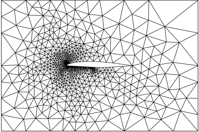
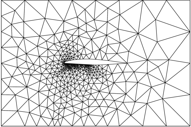
(a)	(b)

Figure 2: Circumcenter vs. off-center insertion on an airfoil model. Smallest angle in both meshes is $32^{\circ}$. Delaunay refinement with circumcenters inserts 731 Steiner points and results in a mesh with 1430 triangles (a). On the other hand, Delaunay refinement with off-centers inserts 441 points and generates a mesh with 854 triangles (b).

Recently, the second author proposed a new insertion strategy for Delaunay refinement algorithm [Üng04]. He introduced the so-called off-centers as an alternative to circumcenters. Off-center of a bad triangle, like circumcenter, is on the bisector of the shortest edge. However, for relatively skinny triangles it is closer to the shortest edge than the circumcenter is. It is chosen such that the triangle formed by the endpoints of the shortest edge and the off-center is barely of good quality. Namely, the off-center insertion is a more “local” operation in the mesh than circumcenter insertion. It is shown in [Üng04] that this new Delaunay refinement algorithm has the same theoretical guarantees as the Ruppert’s refinement, and hence, generates quality-guaranteed size-optimal meshes. Moreover, experimental study indicates that Delaunay refinement algorithm with off-centers inserts considerably fewer Steiner points than the circumcenter insertion algorithms and results in smaller meshes. For instance, when the smallest angle is required to be $32^{\circ}$, the new algorithm inserts about 40% less points and outputs a mesh with about 40% less triangles (see Figure fig:airfoil). This implies substantial reduction not only in mesh generation time, but also in the running time of the application algorithm. This new off-center based Delaunay refinement algorithm is included in the fifth release of the popular Triangle software. Shewchuk observed (personal communication) in this new implementation, that unlike circumcenters, computing off-centers is numerically stable.

Original Delaunay refinement algorithm has quadratic time complexity [Rup93]. This compares poorly to the time-optimal quadtree refinement algorithm of Bern et al. [BEG94] which runs in $O(n\log n+m)$ time, where $m$ is the minimum size of a good quality mesh. The first improvement was given by Spielman et al. [STÜ02] as a consequence of their parallelization of the Delaunay refinement algorithm. Their algorithm runs in $O(m\log m\log^{2}(L/h))$ time (on a single processor), where $L$ is the diameter of the domain and $h$ is the smallest feature in the input. Recently, Miller [Mil04] further improved this describing a new sequential Delaunay refinement algorithm with running time $O((n\log(L/h)+m)\log m)$. In this paper, we present the first time optimal Delaunay refinement algorithm. As Steiner points, we employ off-centers and generate the same output as in [Üng04]. Our improvement relies on avoiding the potentially expensive maintenance of the entire Delaunay triangulation. In particular, we avoid computing very skinny Delaunay triangles, and instead we use a scaffold quadtree structure to efficiently compute, locate and insert the off-center points. Since the new algorithm generates the same output as the off-center based Delaunay refinement algorithm given by Üngör [Üng04], it is still a Delaunay refinement algorithm. In fact, our algorithm implicitly computes the relevant portions of the Delaunay triangulation.

The rest of the paper is organized as follows: In Section sec:pre we survey the necessary background. In Section sec:loose:pairs, we formally define the notion of loose pairs to identify the points that contribute to bad triangles in a Delaunay triangulation. Next, we describe a simple (but not efficient) refinement algorithm based on iterative removal of loose pairs of points. In Section sec:new:alg, we describe the new time-optimal algorithm and prove its correctness. We conclude with directions for future research in Section sec:conclusions.

2 Background

In two dimensions, the input domain $\Omega$ is usually represented as a planar straight line graph (PSLG) — a proper planar drawing in which each edge is mapped to a straight line segment between its two endpoints [Rup93]. The segments express the boundaries of $\Omega$ and the endpoints are the vertices of $\Omega$. The vertices and boundary segments of $\Omega$ will be referred to as the input features. A vertex is incident to a segment if it is one of the endpoints of the segment. Two segments are incident if they share a common vertex. In general, if the domain is given as a collection of vertices only, then the boundary of its convex hull is taken to be the boundary of the input.

The diametral circle of a segment is the circle whose diameter is the segment. A point is said to encroach a segment if it is inside the segment’s diametral circle.

Given a domain $\Omega$ embedded in ${\rm I\!R}^{2}$, the local feature size of each point $x\in{\rm I\!R}^{2}$, denoted by ${\mathrm{lfs}}_{\Omega}(x)$, is the radius of the smallest disk centered at $x$ that touches two non-incident input features. This function is proven [Rup93] to have the so-called Lipschitz property, i.e., ${\mathrm{lfs}}_{\Omega}(x)\leq{\mathrm{lfs}}_{\Omega}(y)+\!\left\|{xy}\right\|$, for any two points $x,y\in{\rm I\!R}^{2}$.

In this extended abstract, we concentrate on the case where $\Omega$ is a set of points in the plane contained in the square $[1/3,2/3]^{2}$. We denote by $P$ the current point set maintained by the refinement algorithm, and by $\mathcal{F}$ the final point set generated.

Let $P$ be a point set in ${\rm I\!R}^{d}$. A simplex $\tau$ formed by a subset of $P$ points is a Delaunay simplex if there exists a circumsphere of $\tau$ whose interior does not contain any points in $P$. This empty sphere property is often referred to as the Delaunay property. The Delaunay triangulation of $P$, denoted $Del(P)$, is a collection of all Delaunay simplices. If the points are in general position, that is, if no $d+2$ points in $P$ are co-spherical, then $Del(P)$ is a simplicial complex. The Delaunay triangulation of a point set can be constructed in $O(n\log n)$ time in two dimensions [Ede01].

In the design and analysis of the Delaunay refinement algorithms, a common assumption made for the input PSLG is that the input segments do not meet at junctions with small angles. Ruppert [Rup93] assumed, for instance, that the smallest angle between any two incident input segment is at least $90^{\circ}$. A typical Delaunay refinement algorithm may start with the constrained Delaunay triangulation [Che89a] of the input vertices and segments or the Delaunay triangulation of the input vertices. In the latter case, the algorithm first splits the segments that are encroached by the other input features. Alternatively, for simplicity, we can assume that no input segment is encroached by other input features. A preprocessing algorithm, which is also parallizable, to achieve this assumption is given in [STÜ02].

For technical reasons, as in [Rup93], we put the input $\Omega$ inside a square $B$. This is to avoid growth of the mesh region and insertion of infinitely many Steiner points. Let $MB=[1/3,2/3]^{2}$ be the minimum enclosing square of $\Omega$. The side length of $B=[0,1]^{2}$ is three times that of $MB$. We insert points on the edges of $B$ to split each into three. This guarantees that no circumcenter falls outside $B$. We maintain this property throughout the algorithm execution by refining the boundary edges as necessary.

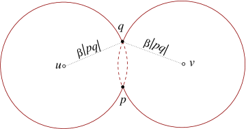
Figure 4: Flower of a pair of points $p$ and $q$.

Radius-edge ratio of a triangle is the ratio of its circumradius to the length of its shortest side. A triangle is considered bad if its radius-edge ratio is larger than a pre-specified constant $\beta\geq\sqrt{2}$. This quality measure is equivalent to other well-known quality measures, such as smallest angle and aspect ratio in two dimensions [Rup93]. Consider a bad triangle, and observe that it must have an angle smaller or equal to $\alpha$, where $\alpha=\arcsin(1/2\beta)$

Table tab:notations (in the appendix) contain a summary of the notation used in this paper.

3 Loose Pairs vs. Bad Triangles

In the following, we use $\beta$ to denote the user specified constant for radius-edge ratio threshold. Accordingly, $\alpha$ denotes the threshold for small angles.

Definition 3.1

For a pair of vertices $p$ and $q$, let $\mathbf{d}_{l}(p,q)$ be the disk with center $u$ such that $pqu$ is a $\mathtt{left\_turn}$ and $\!\left\|{up}\right\|=\!\left\|{uq}\right\|=\beta\!\left\|{pq}\right\|$. Similarly, let $\mathbf{d}_{r}(p,q)$ be the disk with center $v$ such that $pqv$ is a $\mathtt{right\_turn}$ and $\!\left\|{vp}\right\|=\!\left\|{vq}\right\|=\beta\!\left\|{pq}\right\|$. We call the union of the disks $\mathbf{d}_{l}(p,q)$ and $\mathbf{d}_{r}(p,q)$ the flower of $pq$. Moreover, $\mathbf{d}_{l}(p,q)$ is called the left leaf of the flower and $\mathbf{d}_{r}(p,q)$ is called the right leaf of the flower.

A pair of vertices $(p,q)$ in $P$ is a loose pair if either the left or the right leaf of the flower of $pq$ is empty of vertices.

Let $(p,q)$ be a loose pair due to an empty left (resp. right) leaf, and $c$ be the furthest point from $pq$ on the boundary of the leaf. See Figure fig:crescent (a). Let $d$ be the disk centered at $c$ having $p$ and $q$ on its boundary. We call the region $d\setminus\mathbf{d}_{l}(p,q)$ (resp. $d\setminus\mathbf{d}_{r}(p,q)$) the left (resp. right) crescent of $pq$ and denote it by $\mathrm{crescent}_{l}(pq)$ (resp. $\mathrm{crescent}_{r}(pq)$).

Crescent of a loose pair $(p,q)$ may or may not be empty of all the other vertices. In the latter case, the moonstruck of $pq$ is the vertex $r$ inside the crescent such that the circumdisk of $pqr$ is empty of all the other vertices, see Figure fig:crescent (b).

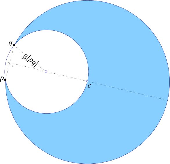
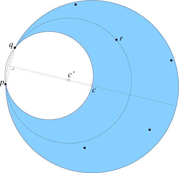
(a)	(b)

Figure 6: The crescent of a loose pair $(p,q)$ is shown as the shaded region (a). If the crescent of $pq$ is empty of all the other vertices then the furthest point from $pq$ inside the leaf (shown as $c$) is the off-center of $pq$. Otherwise, the moonstruck of a loose pair $(p,q)$ with non-empty crescent is shown as $r$ (b). Off-center in this case is the circumcenter of $pqr$, shown as $c^{\prime}$.

Lemma 3.2

There exists a loose pair in a point set $P$ if and only if the minimum angle in the Delaunay triangulation of $P$ is smaller than or equal to $\alpha$.

Proof.

If there exists a loose pair $(p,q)$ then $pq$ is a Delaunay edge. Moreover the triangle incident to edge $pq$ on the side of the empty leaf must be bad, with an angle smaller than $\alpha$.

For the other direction, let $pqr$ be the bad triangle with the shortest edge. Without loss of generality assume $pqr$ is a $\tt{right\_turn}$. If the right leaf of $pq$ is empty then $(p,q)$ is a loose pair and we are done. Otherwise, let $s$ be the first point a morphing from the circumsphere of $pqr$ to right leaf of $pq$ hits (fixing the points $p$ and $q$). Then both $ps$ and $sq$ are shorter features then $pq$ and are incident to a bad Delaunay triangle. This is a contradiction to the minimality of the $\!\left\|{pq}\right\|$. ∎

This lemma suggest the refinement method depicted in Algorithm alg:sequential:basic. Note that each loose pair corresponds to a bad triangle in the Delaunay triangulation of the growing point set. Hence, this algorithm is simply another way of stating the Delaunay refinement with off-centers algorithm presented in [Üng04]. Üngör showed that the Delaunay refinement with off-centers algorithm terminates and the resulting point set is size-optimal. In order to give optimal time bounds we will refine this algorithm in the next section.

Algorithm 2 Loose Pair Removal

0:  A point set $\Omega$ in ${\rm I\!R}^{2}$ and $\beta$

0:  A Steiner triangulation of $\Omega$ where all triangles have radius-edge ratio at most $\beta$

  Let $P=\Omega$

  while there exists a loose pair $(p,q)$ in $P$ do

     Insert the off-center of $pq$ into $P$

  end while

  Compute and Output the Delaunay triangulation of the resulting point set

The next two lemmas follow directly from [Üng04]. They state that during the refinement process we never introduce new features that are smaller than the current loose pair being handled.

Lemma 3.3

Let $P$ be a point-set, $(p,q)$ be a loose pair of $P$, and $P^{\prime}$ be the set resulting for inserting the off-center of $pq$. We have for any $x\in P$, that if ${\mathrm{lfs}}_{P^{\prime}}(x)<{\mathrm{lfs}}_{P}(x)$, then ${\mathrm{lfs}}_{P^{\prime}}(x)\geq\!\left\|{pq}\right\|$.

Lemma 3.4

Let $\Omega$ be the input point set, and let $P$ be the current point set maintained by the refinement algorithm depicted in Algorithm alg:sequential:basic. Let $\mathcal{F}$ denote the point set generated by Algorithm alg:sequential:basic. Then for any point $p$ in the plane, we have throughout the algorithm execution that ${\mathrm{lfs}}_{\Omega}(p)\geq{\mathrm{lfs}}_{P}(p)\geq{\mathrm{lfs}}_{\mathcal{F}}(p)\geq c_{shrink}{\mathrm{lfs}}_{\Omega}(p)$, where $c_{shrink}>0$ is a constant.

Algorithm 4 : Delaunay_Refinement

0:  A point set $\Omega\subseteq[1/3,2/3]^{2}\in{\rm I\!R}^{2}$ and $\beta$

0:  A Steiner triangulation of $\Omega$ where all triangles have radius-edge ratio at most $\beta$

  Split each edge of the square $[0,1]^{2}$ into three segments.

  Construct a balanced quadtree $\mathcal{QT}$ of $\Omega$ using $[0,1]^{2}$ for the root node.

  Insert all the nodes of $\mathcal{QT}$ into a heap $\mathcal{HP}$, sorted from smallest node to largest.

  Initialize all vertices to be active.

  Let $prev\_i$ be the depth of the smallest $\mathcal{QT}$ node.

  while $\mathcal{HP}$ is not empty do

     $\Box\leftarrow\tt{extractMin}(\mathcal{HP})$.

     $i=depth(\Box)$.

     if $i<prev\_i$ then

        Move all vertices in level $prev\_i$ which are also active in level $i$ to the $i$th level.

        $prev\_i=i$.

     end if

     for every active vertex $p\in P\cap\Box$ do

        for every active vertex $q\in P$ such that $\!\left\|{pq}\right\|\leq c_{\mathrm{reach}}\mathrm{size}(\Box)$ do

           if $pq$ is loose then

              Insert the $r=\text{off-center}(p,q)$, and store the $r$ in $\mathcal{QT}$ in a cell ${\Box}^{\prime}$ as low as possible, such that $c_{low}\mathrm{size}({\Box}^{\prime})\leq\!\left\|{pr}\right\|\leq c_{up}\mathrm{size}({\Box}^{\prime})$ and $\mathrm{size}({\Box}^{\prime})\geq\mathrm{size}(\Box)$

           end if

           for every node in the same level of $\Box$ that had a point inserted into it, because of the above step, reinsert it into the heap $\mathcal{HP}$.

        end for

     end for

  end while

  Compute and Output the Delaunay triangulation of the resulting point set

Lemma lemma:fiction suggests a natural algorithm for generating a good cloud of points. Since inserting a new off-center can not decrease the smallest feature of the point cloud, it is natural to first handle the shortest loose pair first. Namely, repeatedly find the smallest loose pair, insert its off-center, till there are no loose pairs left. Because the domain is compact, by a simple packing argument it follows that this algorithm terminates and generates an optimal mesh. This is one possible implementation of (the generic) Algorithm alg:sequential:basic.

Implementing this in the naive way, is not going to be efficient. Indeed, first we need to maintain a heap sorted by the lengths of the loose pairs, which is already too expensive. More importantly, checking if a pair is loose requires performing local queries on the geometry which might be too expensive to perform.

We will overcome these two challenges by handling the loose pairs using a weak ordering on the pairs. This would be facilitated by using a quadtree for answering the range searching queries needed for the loose pairs determination. In particular, our new algorithm is just going to be one possible implementation of Algorithm alg:sequential:basic, and as such Lemma lemma:fiction and Lemma lemma:LFS:the:same hold for it.

4 Efficient Algorithm Using a Quadtree

We construct a balanced quadtree for $\Omega$, using the unit square as the root of the quadtree. In the following, $P$ denotes the current point set, as it grows during the algorithm execution. Let $\mathcal{F}$ be the final point set generated. A balanced quadtree has the property that two adjacent leaves have the same size up to factor two. A balanced quadtree can be constructed, in $O(n\log n+m)$ time, where $m$ is the size of the output, see [BEG94]. Such a balanced quadtree also approximates the local feature size of the input, and its output size $m$ is (asymptotically) the size of the cloud of points we need to generate. In the constructed quadtree we maintain, for each node, pointers to its neighbors in its own level, in the quadtree, and to its neighbors in the levels immediately adjacent to it.

The new algorithm is depicted in Algorithm alg:QT. For the time being, consider all points to be active throughout the execution of the algorithm. Later, we will demonstrate that it is enough to maintain only very few active points inside each cell, thus resulting in a fast implementation. We show that each quadtree node is rescheduled into the heap at most a constant number of times, implying that the algorithm terminates.

In Algorithm alg:QT, collecting the active points around a cell $\Box$, checking whether a pair is active, or finding the moonstruck point of a pair is done by traversing the cells adjacent to the current cell, using the boundary pointers of the well-balanced quadtree. We will show that all those operations takes constant time per cell.

One technicality that is omitted from the description of Algorithm alg:QT, is that we refine the boundary edges of the unit square by splitting such an edge in the middle, if it is being encroached upon. Since the local feature size on the boundary of the unit square is $\Theta(1)$, by Lemma lemma:LFS:the:same. As such, this can automatically handled every time we introduce a new point, and it would require $O(1)$ time for each insertion. This guarantees that no point would be inserted outside the unit square. Note, that in such a case the encroaching new vertex is not being inserted into the point set (although it might be inserted at some later iteration).

4.1 Proof of Correctness

The proof of correctness is by induction over the depth of the nodes being handled. We use $d_{\mathcal{QT}}$ to denote the depth of the quadtree $\mathcal{QT}$. In the $k$th stage of the execution of the algorithm, it handles all nodes of depth $(d_{\mathcal{QT}}-k)$ in the tree. Next, the algorithm handles all nodes of depth $(d_{\mathcal{QT}}-(k+1))$, and so on.

By the balanced quadtree construction [BEG94], for every leaf $\Box$ of the quadtree $\mathcal{QT}$, and every point $p\in P\cap\Box$, we have $c_{low}\mathrm{size}(\Box)\leq{\mathrm{lfs}}_{P}(p)\leq c_{up}\mathrm{size}(\Box)$, where $c_{low}$ and $c_{up}$ are prespecified constants such that $c_{up}\geq 2c_{low}$. In particular, the value of $c_{up}$ and $c_{low}$ is determined by the initially constructed quadtree.

Lemma 4.1

Let $P$ be the current point set maintained by Algorithm alg:QT, and let $r$ be an off-center of a loose pair $(p,q)$ in $P$. Let ${\Box}^{\prime}$ be the quadtree node that the point $r$ is inserted into. We have $c_{low}\cdot\mathrm{size}({\Box}^{\prime})\leq{\mathrm{lfs}}_{P}(r)\leq c_{up}\cdot\mathrm{size}({\Box}^{\prime})$. In particular, $c_{low}^{\prime}\cdot\mathrm{size}({\Box}^{\prime})\leq{\mathrm{lfs}}_{\mathcal{F}}(r)\leq c_{up}\cdot\mathrm{size}({\Box}^{\prime})$, where $c_{low}^{\prime}=c_{shrink}\cdot c_{low}$.

Proof.

The claim follows from the explicit condition used in the insertion part of the algorithm. Observe that since ${\mathrm{lfs}}_{P}(r)=\!\left\|{pr}\right\|\geq{\mathrm{lfs}}_{P}(p)\geq c_{low}\cdot\mathrm{size}(\Box)$, where $\Box$ is the cell of the quadtree containing the point $p$. As such, a node ${\Box}^{\prime}$ that contains $r$ and is in the same level as $\Box$, will have $c_{low}\cdot\mathrm{size}({\Box}^{\prime})\leq{\mathrm{lfs}}_{P}(p)\leq{\mathrm{lfs}}_{P}(r)$, by induction. If ${\mathrm{lfs}}_{P}(r)\leq c_{up}\cdot\mathrm{size}({\Box}^{\prime})$ then we are done. Otherwise, ${\mathrm{lfs}}_{P}(r)>c_{up}\cdot\mathrm{size}({\Box}^{\prime})$ implying that $c_{low}\cdot\mathrm{size}(\mathrm{parent}({\Box}^{\prime}))\leq c_{up}\cdot\mathrm{size}({\Box}^{\prime})\leq{\mathrm{lfs}}_{P}(r)$, since $c_{up}\geq 2c_{low}$. Thus, set ${\Box}^{\prime}\leftarrow\mathrm{parent}({\Box}^{\prime})$ and observe that $c_{low}\cdot\mathrm{size}({\Box}^{\prime})\leq{\mathrm{lfs}}_{P}(r)$, as such we can continue climbing up the quadtree till both inequalities hold simultaneously.

The second part follows immediately from Lemma lemma:LFS:the:same. ∎

Lemma 4.2

Off-center insertion takes $O(1)$ time.

Proof.

Let $r$ be an off-center of a loose pair $(p,q)$, and let $\Box$ and ${\Box}^{\prime}$ be the cells of the quadtree containing $p$ and $r$, respectively. By Lemma lemma:LFS:qt, ${\mathrm{lfs}}_{P}(p)=\Theta(\mathrm{size}(\Box))$. By the algorithm definition, we have $\!\left\|{pq}\right\|=\Theta(\mathrm{size}(\Box))$. As such, $\!\left\|{pr}\right\|=\Theta(\!\left\|{pq}\right\|)=\Theta(\mathrm{size}(\Box))$. Namely, ${\mathrm{lfs}}_{P}(r)=\!\left\|{pr}\right\|=\Theta(\mathrm{size}(\Box))$. Namely, in the grid resolution of $\Box$, the points $p$ and $r$ are constant number of cells away form each other (although $r$ might be stored a constant number of levels above $\Box$). Since every node in the quadtree have cross pointers to its immediate neighbors in its level (or the above level), by the well-balanced property of the quadtree. It follows that we can traverse from $\Box$ to ${\Box}^{\prime}$ using constant time. ∎

Lemma 4.3

The shortest loose pair of $P$ in the beginning of the $i$th stage is of length at least $\eta_{i}=c_{low}^{\prime}/2^{d_{\mathcal{QT}}-i+1}$.

Proof.

For $i=1$, the claim trivially holds by the construction of the balanced quadtree using [BEG94]. Now, assume that the claim holds for $i=1,\ldots,k$. We next show that the claim holds for $i=k+1$. Specifically, it holds at the end of the $k$th stage.

Suppose for the sake of contradiction that there exists a loose pair $(p,q)$ shorter than $\eta_{k}$. Assume, without lose of generality, that $p$ was created after $q$ by the algorithm, and let $\Box$ be the node of $\mathcal{QT}$ that contains $p$. If the depth of $\Box$ is $d_{\mathcal{QT}}-k$, then since $\!\left\|{pq}\right\|\leq\eta_{k}\leq c_{\mathrm{reach}}\mathrm{size}(\Box)$, we have that the algorithm handled the point $p$ in $\Box$, it also considered the pair $(p,q)$ and inserted its off-center. So, the pair $(p,q)$ is not loose at the end of the $k$th stage.

If the depth of $\Box$ is larger then $d_{\mathcal{QT}}-k$ then ${\mathrm{lfs}}(p)$ was larger than $c_{low}\mathrm{size}(\Box)$ when $p$ was inserted. As such, ${\mathrm{lfs}}_{P}(p)>c_{low}^{\prime}\mathrm{size}(\Box)\geq\eta_{k}$, which is a contradiction, since any loose pair that $p$ participates in must be of length at least ${\mathrm{lfs}}_{P}(p)$. ∎

Note that when the algorithm handles the root node in the last iteration, it “deteriorates” into being Algorithm alg:sequential:basic executed on the whole point set. Hence Lemma lemma:inductive implies the following claim.

Claim 4.4

In the end of the execution of Algorithm alg:QT, there are no loose pairs left in $\mathcal{F}$, where $\mathcal{F}$ is the point set generated by the algorithm.

4.2 How the refinement evolves

Our next task, is to understand how the refinement takes place around a point, and form a “protection”area around it. In particular, the region around a point $p\in P$ with ${\mathrm{lfs}}_{\Omega}(p)$ is going to be effected (i.e., points inserted into it), starting when the algorithm handles cells of level $i$, where $1/2^{i}\approx{\mathrm{lfs}}_{\Omega}(p)$. Namely, the region around $p$ might be refined in the next few levels. However, after a constant number of such levels, the point $p$ is surrounded by other points, and $p$ is not loose with any of those points. As such, the point $p$ is no longer a candidate to be in a loose pair. To capture this intuition, we prove that this encirclement process indeed takes place.

We define the gap of a vertex $x\in P$ (which is not a boundary vertex), denoted by $\mathrm{gap}(x)$, as the ratio between the radius of the largest disk that touches $x$ and does not contain any vertex inside, and the ${\mathrm{lfs}}_{P}(x)$.

Lemma 4.5

For a vertex $w\in P$, if $\mathrm{gap}(w)>c_{g}=(2\beta)^{\pi/\alpha+1}$, then there exists a loose pair of $P$ of length $\leq c_{gbu}\cdot{\mathrm{lfs}}(w)$, where $c_{gbu}=(2\beta)^{\pi/\alpha}$.

Proof.

Assume that $w$ is strictly inside the bounding square $B$. Proof for the case where $w$ is on the boundary of $B$ is similar and hence omitted. Let $T_{1},T_{2},\ldots,T_{m}$ be the Delaunay triangles incident to $w$ and $u_{1},u_{2},\ldots,u_{m}$ be the Delaunay neighbors of $w$. Note that if $\!\left\|{wu_{i}}\right\|\geq 2\beta\!\left\|{wu_{i-1}}\right\|$, then the left flower of $wu_{i-1}$ must be empty and hence $wu_{i-1}$ is a loose pair. Similarly, if $\angle{wu_{i}u_{i-1}}<\alpha$ then $(w,u_{i-1})$ is a loose pair. If $\angle{wu_{i}u_{i-1}}\geq\alpha$ and $\angle{u_{i}wu_{i-1}}<\alpha$ then by the law of sines, it must be that $\!\left\|{u_{i}u_{i-1}}\right\|\leq\!\left\|{u_{i-1}w}\right\|$, and $u_{i}u_{i-1}$ is facing an angle smaller than $\alpha$, and as such it is a loose pair.

Suppose that none of the triangles $T_{1},\ldots,T_{m}$ have a loose pair on their boundary. Then, it must be that $m\leq 2\pi/\alpha$, since the angle $\angle u_{i}wu_{i+1}\geq\alpha$, for $i=1,\ldots,m$. But then, $\!\left\|{u_{i}w}\right\|\leq(2\beta)^{i-1}{\mathrm{lfs}}(w)$ and $\!\left\|{u_{i}w}\right\|\leq(2\beta)^{m-i+1}{\mathrm{lfs}}(w)$. It follows that $\!\left\|{u_{i}w}\right\|\leq(2\beta)^{\pi/\alpha}{\mathrm{lfs}}(w)$, for $i=1,\ldots,m$. Since, all the angles in $T_{i}$ are larger than $\alpha$, it follows that circumcircle of $T_{i}$ is of radius $\leq\beta\!\left\|{u_{i}w}\right\|\leq\beta(2\beta)^{\pi/\alpha}{\mathrm{lfs}}(w)$. But then, the gap around $w$, is at most $\beta(2\beta)^{\pi/\alpha}$. A contradiction, since $\mathrm{gap}(w)=c_{g}>\beta(2\beta)^{\pi/\alpha}$.

Thus, one $T_{1},\ldots,T_{m}$ must be bad. Arguing as above, one can show that the first such triangle, has a loose pair of length $\leq(2\beta)^{\pi/\alpha}{\mathrm{lfs}}(w)$, as claimed. ∎

Lemma lemma:gap implies that if we handle all loose pairs of length smaller than $\ell$, then all the points having a big gap, must be with local feature size $\Omega(\ell)$.

Lemma 4.6

Let $P$ be a point set such that all the loose pairs are of length at least $\ell/c_{1}$, for a constant $c_{1}\geq 2$. Let $(p,q)$ be a loose pair of length $\ell$ with a non-empty crescent, and let $w$ be its moonstruck neighbor. Then, ${\mathrm{lfs}}(w)\geq\frac{\ell}{c_{1}c_{gbu}}$.

Proof.

Since $w$ is a moonstruck point of a loose pair of length at least $\ell$ there is an empty ball of radius at least $\beta\ell$ touching $w$. Hence, $\mathrm{gap}(w)\geq\frac{\beta\ell}{{\mathrm{lfs}}(w)}$. We consider two cases. If $\frac{\beta\ell}{{\mathrm{lfs}}(w)}\geq c_{g}$, then by Lemma lemma:gap, there exist a loose pair of size at most $c_{gbu}{\mathrm{lfs}}(w)$. However, all loose pairs are of length $\geq\ell/c_{1}$, and it follows that $c_{gbu}{\mathrm{lfs}}(w)\geq\ell/c_{1}$. Hence, ${\mathrm{lfs}}(w)\geq\ell/(c_{1}c_{gbu})$. On the other hand, if $\frac{\beta\ell}{{\mathrm{lfs}}(w)}\leq c_{g}$ then,

$${\mathrm{lfs}}(w)\geq\frac{\beta\ell}{c_{g}}\geq\frac{\ell}{c_{g}}\geq\frac{\ell}{c_{gbu}}\geq\frac{\ell}{c_{1}c_{gbu}},$$

since $c_{gbu}\geq c_{g}$ and $\beta\geq 1$. ∎

4.3 Managing Active Points

As we progress with execution of the algorithm, the results of the previous section imply that a vertex with relatively small feature size cannot participate in a loose pair, nor be a moonstruck point. So, in the evolving quadtree we do not maintain such set of points that play no role in the later stages of the algorithm execution. This facilitates an efficient search for finding the loose pairs and moonstruck points as shown in the rest of this section. For each vertex, size of its insertion cell gives a good approximation of its feature size. We use this to determine the lifetime of each vertex in our evolving quadtree data structure.

The activation depth of an input vertex $p$, denoted by ${\overline{p}}$, is the level of the initial quadtree leaf containing $p$. For a Steiner point $p$, the activation depth is the depth of the cell $p$ is inserted into.

Lemma 4.7

A vertex $p$ can not be a loose pair end or a moonstruck point, when the algorithm handles level of depth $<{\overline{p}}-c_{\mathrm{span}}$, where $c_{\mathrm{span}}=\lg\frac{c_{gbu}c_{up}}{c_{low}^{\prime}}+1$.

Proof.

When the point $p$ was created, we had ${\mathrm{lfs}}_{P}(p)\leq c_{up}/2^{\overline{p}}$, by Lemma lemma:LFS:qt. Now, if $p$ is an endpoint of a loose pair in depth $m\leq{\overline{p}}$ in the quadtree, it must be that the length $\ell$ of this pair is at least $c_{low}^{\prime}/2^{m}$, by Lemma lemma:inductive. Since the local feature size ${\mathrm{lfs}}_{P}$ is a non-increasing function as our algorithm progresses, it follows that

$$\mathrm{gap}(p)\geq\frac{\ell}{{\mathrm{lfs}}_{P}(p)}\geq\frac{c_{low}^{\prime}/2^{m}}{c_{up}/2^{\overline{p}}}=2^{{\overline{p}}-m}\cdot\frac{c_{low}^{\prime}}{c_{up}}.$$

If $\mathrm{gap}(p)\leq c_{g}$ then $2^{{\overline{p}}-m}\cdot\frac{c_{low}^{\prime}}{c_{up}}\leq c_{g}$. Implying that ${\overline{p}}-m\leq\lg\frac{c_{g}c_{up}}{c_{low}}$.

By Lemma lemma:gap, if $\mathrm{gap}(p)$ at any point in the algorithm becomes larger than $c_{g}$, then there exists a loose pair of length $\leq c_{gbu}\cdot{\mathrm{lfs}}_{P}(p)$. But all such pairs are handled in level $\geq\mathsf{t}$ in the quadtree, where $c_{gbu}\cdot{\mathrm{lfs}}_{P}(p)\geq c_{low}^{\prime}/2^{\mathsf{t}+1}$ by Lemma lemma:inductive. Thus, $c_{gbu}c_{up}/2^{\overline{p}}\geq c_{gbu}{\mathrm{lfs}}_{P}(p)\geq c_{low}^{\prime}/2^{\mathsf{t}+1}$. Implying that

$$\mathsf{t}\geq\rho={\overline{p}}-\lg\frac{c_{gbu}c_{up}}{c_{low}^{\prime}}-1.$$

This implies, that when the algorithm handles cells of depth $1,\ldots,\rho$, we have that the vertex $p$ can not participate directly in a loose pair.

If $p$ is not loose pair end, but is a moonstruck point for a loose pair, then

$$\frac{c_{up}}{2^{\overline{p}}}\geq{\mathrm{lfs}}_{P}(p)\geq\frac{c_{low}^{\prime}}{2^{\mathsf{t}+1}c_{gbu}}$$

by Lemma lemma:moonstruck and Lemma lemma:inductive. This in turn implies that $\mathsf{t}\geq{\overline{p}}-\lg\frac{c_{gbu}c_{up}}{c_{low}^{\prime}}-1$. ∎

Definition 4.8

A point $p$ is active at depth $i$, if ${\overline{p}}\geq i\geq{\overline{p}}-c_{\mathrm{span}}$, where $c_{\mathrm{span}}$ is a constant specified in Lemma lemma:life:span.

Note, that the algorithm can easily maintain the set of the active points. Lemma lemma:life:span implies that only active points are needed to be considered in the loose pair computation.

Observation 4.9

During the off-center insertion any new loose pairs introduced are at least the size of the existing loose pairs.

Lemma 4.10

At any stage $i$, the number of active points inside a cell at level $d_{\mathcal{QT}}-i$ is a constant.

Proof.

This is trivially true in the beginning of the execution of the algorithm, as the initial balanced quadtree has at most a constant number of vertices in each leaf. Later on, Lemma lemma:life:span implies that when a point $p$ is being created, with $\ell={\mathrm{lfs}}(p)$, then its final local feature size is going to be $\Theta(\ell)$. To see that, observe that when $p$ was created, the algorithm handled loose pairs of size $\Omega(\ell)$. From this point on, the algorithm only handle loose pairs that are longer (or slightly shorter) than $\ell$. Such a loose pair, can not decrease the local feature size to be much smaller than $\ell$, by Lemma lemma:fiction.

This implies that when $p$ is being created, we can place around it a ball of radius $\Omega({\mathrm{lfs}}(p))$ which would contain only $p$ in the final generated point set. Since $p$ becomes inactive $c_{\mathrm{span}}$ levels above the level it is being created, it follows that a call in the quadtree can contain at most a constant number of such protecting balls, by a simple packing argument. ∎

4.4 Efficient Implementation Details

The above discussion implies that during the algorithm execution, we can maintain for every quadtree node a list of constant size that contains all the active vertices inside it. When processing a node, we need to extract all the active points close to this cell $\Box$. This requires collecting all the cells in this level, which are constant number of cells away from $\Box$ in this grid resolution. In fact, the algorithm would do this point collection also in a constant number of levels above the current level, so that it collects all the Steiner points that might have been inserted. Since throughout the execution of the algorithm we maintain a balanced quadtree, we have from every node, pointers to its neighbors either in its level, or at most one level up. As such, we can collect all the neighbors of $\Box$ in constant distance from it in the quadtree, in constant time, and furthermore, extract their active points in constant time. Hence, handling a node in the main loop of Algorithm alg:QT takes constant time.

We need also to implement the heap used by the algorithm. We store nodes in the heap $\mathcal{HP}$, and it extracts them according to their depth in the quadtree. As such, we can implement it by having a separate heap for each level of the quadtree. Note that the local feature size of a vertex when inserted into a quadtree node is within a constant factor of the size of the node. Hence a node can be rescheduled in the heap at most a constant number of times. For each level, the heap is implemented by using a linked list and a hash-table. Thus, every heap operation takes constant time.

4.5 Connecting the Dots

We shall also address how to perform the final step of Algorithm alg:QT, that is computing the Delaunay triangulation of the resulting point set $\mathcal{F}$. This can be done by re-executing a variant of the main loop of Algorithm alg:QT on $\mathcal{F}$, which instead of refining the point set, reports the Delaunay triangles. We use a similar deactivation scheme to ignore vertices whose all Delaunay triangles are reported. Since $\mathcal{F}$ is a well-spaced point set, for a pair of nearby active vertices we can efficiently compute whether the two makes a Delaunay edge and if so locate also the third point that would make the Delaunay triangle. It is straightforward but tedious to argue that the running time of this algorithm is going to be proportional to the running time of Algorithm alg:QT.

4.6 Analysis

The initial balanced quadtree construction takes $O(n\log n+m)$ time, where $m$ is the size of the resulting quadtree [BEG94]. This quadtree has the property that the size length of a leaf is proportional to the local feature size. This in turn implies the value of $c_{low}$ and $c_{up}$, which in turn guarantees that no new leafs would be added to the quadtree during the refinement process.

Furthermore, the point set generated by Algorithm alg:QT has the property that its density is proportional to the local feature size of the input. Namely, the size of the generated point-set is $O(m)$. Since all the operations inside the loop of Algorithm alg:QT takes constant time, we can charge them to either the newly created points, or to the relevant nodes in the quadtree. This immediately implies that once the quadtree is constructed, the running time of the algorithm is $O(m)$.

Theorem 4.11

Given a set $\Omega$ of $n$ points in the plane the Delaunay refinement algorithm (depicted in Algorithm alg:QT) computes a quality-guaranteed size-optimal Steiner triangulation of $\Omega$, in optimal time $O(n\log n+m)$, where $m$ is the size of the resulting triangulation.

5 Conclusions

We presented a time-optimal algorithm for Delaunay refinement in the plane. It is important to note that the output of this new algorithm is the same as that of the off-center based Delaunay refinement algorithm given in [Üng04], which outperforms the circumcenter based refinement algorithms in practice. The natural open question for further research is extending the algorithm in three (and higher) dimensions. We believe that extending our algorithm to handle PSLG in the plane is doable (with the same time bounds), but is not trivial, and it would be included in the full version of this paper.

We note that when building the initial quadtree, we do not have to perform as many refinement steps as used in the standard quadtree refinement algorithm of Bern et al. [BEG94]. While their algorithm considers a quadtree cell with two input vertices crowded and splits it into four, we are perfectly satisfied with a balanced quadtree as long as the quadtree approximates the local feature size within a constant and hence the number of features in a cell is bounded by a constant. This difference in the depth of the quadtree should be exploited for an efficient implementation of our algorithm (this effects the values of the constants $c_{low}$ and $c_{up}$).

Parallelization of quadtree based methods are well understood [BET99], while design of a theoretically optimal and practical parallel Delaunay refinement algorithm is an ongoing research topic [STÜ02, STÜ04]. We believe our approach of combining the strengths of quadtrees as a domain decomposition scheme and Delaunay refinement with off-centers will lead to a good parallel solution for the meshing problem.

Notation Value Comment $\Omega$ Input point set. $P$ Current point set maintained by the algorithm. $\mathcal{F}$ Final point set $\beta$ $\geq\sqrt{2}$ radius-edge ratio threshold for bad triangles $\alpha$ $\arcsin(1/2\beta)$ small angle threshold bad triangles $c_{g}$ $(2\beta)^{\pi/\alpha+1}$ Vertex with larger gap than $c_{g}$ participates in a loose pair. $c_{gbu}$ $(2\beta)^{\pi/\alpha}$ Blowup of ${\mathrm{lfs}}$ for a lose pair around a vertex with large gap. $c_{low}$ Lower bound on the ${\mathrm{lfs}}$ of a point inside a leaf of the initial quadtree. $c_{up}$ $\geq 2c_{low}$ Upper bound on the ${\mathrm{lfs}}$ of a point inside a leaf of the quadtree. $c_{\mathrm{reach}}$ $2c_{up}c_{gbu}$ $c_{\mathrm{reach}}\mathrm{size}(\Box)$ is an upper bound on the length of a (relevant) lose pair involving a point $p$ stored in a cell $\Box$. For correctness, it required that $c_{\mathrm{reach}}\geq 2\sqrt{2}$. $c_{shrink}$ $>0$ For any point $x$, we have ${\mathrm{lfs}}_{\mathcal{F}}(x)\geq c_{shrink}\cdot{\mathrm{lfs}}_{\Omega}(x)$. $c_{low}^{\prime}$ $c_{low}\cdot c_{shrink}$ Lower bound on the ${\mathrm{lfs}}$ of a point $p$ stored inside a node $\Box$ of the quadtree through the algorithm execution. Namely, ${\mathrm{lfs}}_{\mathcal{F}}(p)\geq c_{low}^{\prime}\mathrm{size}(\Box)$.

Table 2: Notation used in the paper.

References

- [BEG94] M. Bern\Hy@xspace@end, D. Eppstein\Hy@xspace@end, and J. Gilbert. Provably good mesh generation. J. Comput. Syst. Sci., 48:384–409, 1994.
- [BET99] M. Bern\Hy@xspace@end, D. Eppstein\Hy@xspace@end, and S.-H. Teng. Parallel construction of quadtrees and quality triangulations. Internat. J. Comput. Geom. Appl., 9(6):517–532, 1999.
- [Che89a] L. P. Chew. Constrained Delaunay triangulations. Algorithmica, 4:97–108, 1989.
- [Che89b] L. P. Chew. Guaranteed-quality triangular meshes. Technical Report TR-89-983, Dept. Comput. Sci., Cornell Univ., Ithaca, NY, April 1989.
- [DBS92] T. K. Dey, C. L. Bajaj, and K. Sugihara. On good triangulations in three dimensions. Internat. J. Comput. Geom. Appl., 2(1):75–95, 1992.
- [Ede01] H. Edelsbrunner\Hy@xspace@end. Geometry and Topology for Mesh Generation\Hy@xspace@end. Cambridge Univ. Press, 2001.
- [EG01] H. Edelsbrunner\Hy@xspace@end and D. Guoy. Sink insertion for mesh improvement. In Proc. ACM Symp. Comp. Geom., pages 115–123, 2001.
- [Loh96] R. Lohner. Progress in grid generation via the advancing front technique. Engineering with Computers, 12:186–210, 1996.
- [Mil04] G. L. Miller. A time efficient Delaunay refinement algorithm. In Proc. 15th ACM-SIAM Sympos. Discrete Algorithms, pages 400–409, 2004.
- [MPW03] G. L. Miller, S. Pav, , and N. Walkington. When and why Ruppert’s algorithm works. In Proc. th Int. Meshing Roundtable, pages 91–102, 2003.
- [MV00] S. A. Mitchell and S. A. Vavasis. Quality mesh generation in higher dimensions. SIAM J. Comput., 29:1334–1370, 2000.
- [Rup93] J. Ruppert. A new and simple algorithm for quality 2-dimensional mesh generation. In Proc. 4th ACM-SIAM Sympos. Discrete Algorithms, pages 83–92, 1993.
- [SF73] G. Strang and G. Fix. An Alaysis of the Finite Element Method. Prentice Hall, Englewood Cliffs, NJ, 1973.
- [She97] J. R. Shewchuk. Delaunay Refinement Mesh Generation\Hy@xspace@end. PhD thesis, Carnegie Mellon University, 1997.
- [STÜ02] D. A. Spielman, S.-H. Teng, and A. Üngör\Hy@xspace@end. Parallel Delaunay refinement: Algorithms and analyses. In Proc. th Int. Meshing Roundtable, pages 205–217, 2002.
- [STÜ04] D. A. Spielman, S.-H. Teng, and A. Üngör\Hy@xspace@end. Time complexity of practical parallel Steiner point insertion algorithms. In Proc. 16th ACM Sympos. Parallel Alg. Arch., pages 267–268, 2004.
- [Üng04] A. Üngör\Hy@xspace@end. Off-centers: A new type of steiner points for computing size-optimal quality-guaranteed delaunay triangulations. In Latin Amer. Theo. Inf. Symp., pages 152–161, 2004.