The vertex-transitive
TLF-planar graphs

David Renault
renault@labri.fr
LaBRI – Université Bordeaux I
351, cours de la Libération
33400 Talence, France
Abstract

We consider the class of the topologically locally finite (in short TLF) planar vertex-transitive graphs, a class containing in particular all the one-ended planar Cayley graphs and the normal transitive tilings. We characterize these graphs with a finite local representation and a special kind of finite state automaton named labeling scheme. As a result, we are able to enumerate and describe all TLF-planar vertex-transitive graphs of any given degree. Also, we are able decide to whether any TLF-planar transitive graph is Cayley or not.

Keywords: vertex-transitive, planar graph, tiling, topologically locally finite, labeling scheme

Introduction

Vertex-transitive graphs – or transitive graphs in short – are graphs whose group of automorphisms acts transitively on their sets of vertices. These graphs possess a regular structure, being structurally the same from any vertex. When such a graph is planar, this regular structure confers symmetry properties to the embedding of the graph : the action of automorphisms on the graph can locally be represented as the action of an isometry of the geometry it is embedded in.

The class $\mathcal{T}$ of the topologically locally finite (in short TLF) planar transitive graphs is a subclass of the class of the transitive planar graphs. These graphs possess a planar embedding such that the set of vertices in this embedding is a locally finite subset of the plane. For example, $\mathcal{T}$ contains the planar Cayley graphs of the discrete groups of isometries of the plane, be it hyperbolic or Euclidean. We find in $\mathcal{T}$ both tree-like graphs of finite treewidth and one-ended graphs such as the Euclidean grid.

The TLF-planar graphs are related to several fields: first, such graphs represent adapted models of computation for parallel algorithms such as cellular automata MD (98); Gar (95), and provide examples of structures for interconnection networks HD (97). The class $\mathcal{T}$ is also connected to the vertex-transitive tilings of the plane whose set of vertices is topologically locally finite GS (87). Second, while many problems in combinatorial group theory are undecidable, the planar vertex-transitive graphs possess structural as well as geometrical properties that allow for a more specific approach. For example, the unique embedding property in the case of the 3-connected planar graphs Whi (32) constrains the structure of the automorphisms of the graph. Finally, putting aside the finite graphs in $\mathcal{T}$, the infinite graphs in $\mathcal{T}$ may factor into finite transitive graphs embedded into compact manifolds, as it is the case for Euclidean graphs Wol (84).

The characterization of the finite planar transitive graphs is a result of Fleischner and Imrich FI (79). These graphs turn out to be the complexes associated to the uniform convex polyhedra. The finite non-planar case happens to be much more difficult, and has been thoroughly studied up to 26 vertices by McKay et al. MR (90); Roy (97), but few general results are known. Cayley graphs are natural examples of vertex-transitive graphs, and McKay also studied the problem of the determination of those graphs that were transitive but not Cayley graphs MP (94, 96). The problem of enumerating the normal Cayley graphs, has been solved by Chaboud Cha (95) and then extended to the TLF-planar Cayley graphs Ren (03).

In this paper, we give an exhaustive description of the class $\mathcal{T}$ of the TLF-planar vertex-transitive graphs. Our description of the class includes both finite and infinite graphs. This extends the Cayley case Ren (03) in several ways. First, the Cayley case is mainly dedicated to the description of groups which happen to have a planar Cayley graph. This article focuses on the graphs themselves, by describing all their possible groups of automorphisms, and as a consequence all their possible embeddings. Second, we can highlight properties of the transitive graphs that do not hold when we restrict ourselves to Cayley graphs. For example, TLF-planar Cayley graphs can always be represented by the Cayley graph of a discrete group of isometries of the plane. There exist transitive graphs for which this is impossible, independently of the embedding. Finally, $\mathcal{T}$ contains a strictly larger class of graphs than the Cayley case. Such a simple graph as the complex associated to the dodecahedron is an example of transitive but non Cayley planar graphs. More precisely, there exist infinite families of graphs having this property.

In this article, we refine the description of the groups of automorphisms of the graphs and the geometrical properties of their possible planar embeddings given in Ren (03). We represent these graphs by their geometrical invariants in a structure called a labeling scheme, as long as a special kind of finite state automaton called a border automaton. We show that there exists a bijection between this representation and the class of the TLF-planar transitive graphs. Our main result (page 15) is:

Theorem 15 (Enumeration) Given a number $d\geq 2$, it is possible to enumerate all the TLF-planar transitive graphs having internal degree $d$, along with their labeling schemes.

Each vertex-transitive graph belonging to the class $\mathcal{T}$ is effectively computable (i.e. there exists an algorithm able to build every finite ball of the graph). Associated to our results on Cayley graphs, this allows us to determine which of these graphs are Cayley, and more precisely:

Corollary 16 (Cayley checking) If $\Gamma$ is a TLF transitive graph, then it is decidable whether $\Gamma$ is the Cayley graph of a group or not, and obtain an enumeration and a description of the groups having $\Gamma$ as a Cayley graph.

Finally, thanks to the characterization of the embeddings of the graphs in $\mathcal{T}$, it is possible to compute their connectivity and approximate their growth rate, which can be either linear, quadratic or exponential, depending on their local geometrical properties.

1 TLF-planar transitive graphs

A graph $\Gamma$ consists of a pair $(V,E)$, $V$ being a countable set of vertices and a set of edges, where $E$ is a subset of the pair of elements of $V$. Each edge corresponds to a pair of vertices $(v_{1},v_{2})$ called its extremities. An edge with the same extremities $(v,v)$ is called a loop. The graphs that we consider are loopless. An edge $(u,v)$ is said to be incident to the vertices $u$ and $v$. A labeling of the graph is an application from the set of edges into a finite set $L$ of labels or colors. The degree of a vertex is the number of edges incident to this vertex. A path of $\Gamma$ is a sequence of vertices $(v_{n})$ in $\Gamma$ such that for all $n$, there exists an edge between $v_{n}$ and $v_{n+1}$. A cycle is a finite path whose initial and terminal vertices are the same. A simple cycle is a cycle where no vertex appears twice.

Remark 1 –

Considerations on the construction of subgraphs We occasionally build subgraphs of $\Gamma$ by considering a certain subset of vertices and edges $(V^{\prime},E^{\prime})$ where $V^{\prime}\subset V$ and $E^{\prime}\subset E$, or equivalently by removing from the graph a subset of its vertices and edges. Then, we can consider the remaining set of vertices and edges as a subspace of the graph seen as a metric space, and the connected components of this subspace. These components may not be graphs themselves, since some edges will not have vertices as their extremities. We can resolve this problem and consider these components as new graphs by adding new vertices to the extremities of these edges.  

A graph $\Gamma$ is connected if, for every pair of vertices $(s_{1},s_{2})$ of the graph, there exists a finite path in the graph with extremities $s_{1}$ and $s_{2}$. A connected component is an equivalence class of vertices for the relation “to be connected”. Notice that both definitions are coherent whether $\Gamma$ is seen as a graph or as a metric space. A n-separation is a set of $n$ vertices whose removal separates the graph in two or more connected components not reduced to a single edge. A cut-vertex of $\Gamma$ is a $1$-separation of $\Gamma$. A graph is $n$-separable if it contains a $n$-separation. If it contains no $n$-separation, it is (n+1)-connected. A graph is regular when all its vertices have the same degree $d$. The graphs we will be dealing with are connected and regular.

A morphism from the graph $\Gamma_{1}=(V_{1},E_{1})$ into $\Gamma_{2}=(V_{2},E_{2})$ is an application $\sigma:V_{1}\rightarrow V_{2}$ that preserves the edges of the graph. When both graphs are labeled, we impose that the morphisms also preserve the labels of the edges. A graph is said to be vertex-transitive – or transitive in short – if and only if, given any two vertices $(s_{1},s_{2})\in\Gamma$, there exists an automorphism of $\Gamma$ mapping $s_{1}$ onto $s_{2}$. If $\Gamma$ is the Cayley graph of a group, then it is vertex-transitive.

Remark 2 –

About the lower degree transitive graphs There exists only one non-trivial connected transitive graph of degree $1$, which corresponds to $K_{2}$, the graph reduced to a single edge. Transitive graphs of degree $2$ correspond to cyclic graphs $C_{n}$ where $n$ may be infinite. These graphs possess exactly one labeling when $n$ is odd and two labelings when $n$ is even, these labelings corresponding to the planar Cayley graphs of degree $2$ associated to the dihedral groups and cyclic groups. In the following, we shall only be interested in connected transitive graphs of degree $d\geq~{}3$.  

A graph $\Gamma$ is said to be planar if it can be embedded in the plane, such that no two edges meet in a point other than a common end. By the plane, we mean a simply connected Riemannian surface, homogeneous and isotropic. For our embeddings, we will only consider the three usual geometries : the sphere, the Euclidean and the hyperbolic plane. Our embeddings will be considered tame, meaning that all edges are $\mathcal{C}^{1}$ images of $[0;1]$. Such an embedding is said to be topologically locally finite – in short TLF-planar – if its vertices have no accumulation point in the plane. Equivalently, every compact subset of the plane intersects a finite number of vertices of the embedding. Symmetrically, an embedding is said to be TLF in terms of edges if and only if every compact subset of the plane intersects a finite number of edges of the embedding. The following theorem asserts that a TLF-planar graph always possess such an embedding:

Theorem 3 (Ren (03)).

If the graph $\Gamma$ is TLF-planar, there exists a tame embedding of the same graph that is TLF in terms of vertices but also of edges.

We will always suppose that the TLF-planar graphs are embedded in the plane such that their embedding follows Theorem 3. Given a specific embedding of a TLF-planar graph $\Gamma$, a face $\mathcal{F}$ is defined as an arc-connected component of the complement of the graph in the plane. $\mathcal{F}$ is said to be finite when it is incident to finitely many vertices of the graph, otherwise it is said to be infinite. For TLF-planar graphs, infinite faces are necessarily topologically unbounded in the plane. The border of the face $\mathcal{F}$, noted $\partial\mathcal{F}$, is its boundary in topological terms. A face $\mathcal{F}$ is said to be incident to a vertex or an edge of the graph if and only if this vertex of edge intersects with $\partial\mathcal{F}$.

In such an embedding, every edge incident to a face is entirely included into the border of this face. Then every edge is incident to exactly two faces of $\Gamma$, which it separates. Considering the previous definitions of the faces, the transitivity property of $\Gamma$ stands out with the following lemma taken from Ren (03):

Lemma 4 (Intersection of faces).

Let $\Gamma$ be a vertex-transitive TLF-planar graph. Given two distinct faces of $\Gamma$, the intersection of their border, when non-empty, is either a vertex or an edge of $\Gamma$.

Corollary 5 (Preservation of finite faces).

The automorphisms of $\Gamma$ map the border of every finite face onto the border of another finite face.

Remark 6 –

On the choice of the embedding The previous statements hold for a particular embedding of $\Gamma$ that is locally finite in terms of edges and vertices. This embedding may not be unique. For example, if $\Gamma$ is finite, there exists an embedding of $\Gamma$ in the sphere, where all faces are topologically bounded. If we select a point inside a face and send this point to the infinity, we obtain another embedding of the graph on a non-compact surface homeomorphic to the Euclidean plane. With the previous definitions, the faces of both embeddings are all finite, and the validity of Corollary 5 is the same for both embeddings.  

The size of a face of an embedding of $\Gamma$ corresponds to the number (possibly infinite) of vertices it is incident to. The type vector of a vertex of $\Gamma$ is the sequence of sizes of the faces appearing consecutively around this vertex. It is defined up to rotation and symmetry of the graph. If $\Gamma$ is transitive and Corollary 5 holds, the type vector is independent of the choice of the vertex, up to permutation of its elements. For example, the type vector of the Euclidean infinite grid is $[4;4;4;4]$ and the type vector of a cyclic graph $C_{n}$ with $n$ vertices is $[n;n]$.

For a given graph $\Gamma$, $\textrm{Aut}(\Gamma)$ denotes its group of automorphisms, and $\textrm{Trans}(\Gamma)$ stands for the set of subgroups of $\textrm{Aut}(\Gamma)$ acting transitively on the set of vertices of $\Gamma$. Let $G$ belong to $\textrm{Trans}(\Gamma)$. $G$ acts on the set of edges of $\Gamma$ and the set of orbits of edges is finite. Thus a class or a color of edges is defined as an orbit under the action of $G$, the set of colors being called $\mathsf{E}_{G}$. In the same manner, we define classes or colors of finite faces, corresponding to the finite set $\mathsf{F}_{G}$. This coloring defines a partition of the set of finite faces of the embedding. Infinite faces have a special status since these faces may not be stable by automorphism. Therefore, we request by convention that all of them correspond to a special color in $\mathsf{F}$.

In the following, $\Gamma$ will be a TLF-planar, connected vertex-transitive graph of finite degree $d\geq 3$. Thus we will speak of vertices, edges and faces of $\Gamma$, as defined above. $G$ is a group belonging to $\textrm{Trans}(\Gamma)$. We will always suppose that the embedding of $\Gamma$ follows Theorem 3 and that the automorphisms preserve the borders of the finite faces. In the section 2, we analyze these local invariants, in order to obtain a characterization of the graph by its local geometrical properties in section 3. The last section presents some applications of these characterizations.

2 Local geometrical invariants

2.1 Infinite faces and connectivity

Let us give some intuition on the general structure of the graphs in this class. We prove that the finite vertex-transitive planar graphs of degree $\geq 3$ are all $3$-connected graphs, and in the infinite case, the connectivity of the graphs depends only on the number of infinite faces appearing around each vertex:

Lemma 7 (Connectivity and infinite faces).

If $\Gamma$ is a TLF-planar transitive graph of degree $\geq 3$, let $n$ be the number of infinite faces appearing around a given vertex of $\Gamma$. Then, depending on the value of $n$:

  • $n\geq 2\Leftrightarrow\Gamma$ is 1-separable.

  • $n=1\Leftrightarrow\Gamma$ is 2-connected and 2-separable;

  • $n=0\Leftrightarrow\Gamma$ is 3-connected;

$n=0$ $n=1$ $n\geq 2$

Proof 1 –
  • ($n\geq 2\Leftrightarrow\Gamma$ is $1$-separable)
    Given a vertex $v$ of $\Gamma$, we consider the set of faces incident to that vertex, and the union of the borders of those faces that are finite. If $n\geq 2$, the union of $v$ and two infinite faces incident to $v$ separates the graph into at least two non-trivial components. Then every vertex of the graph is a cut-vertex and the graph is $1$-separable. On the other hand, if $\Gamma$ is $1$-separable, every vertex must meet at least $2$ infinite faces.

  • ($n=1\Rightarrow\Gamma$ is $2$-connected and $2$-separable)
    If $n=1$, then consider an edge of $\Gamma$ that does not belong to the border of an infinite face. There must exist one, otherwise $\Gamma$ being of degree at least $3$, that would contradict the fact that $n=1$. The extremities of this edge both meet an infinite face, and these faces are distinct. The removal of these extremities separates $\Gamma$, therefore $\Gamma$ is 2-separable. It is $2$-connected because $n<2$.

  • ($\Gamma$ is $2$-connected and $2$-separable $\Rightarrow n=1$)
    Suppose now that $\Gamma$ is $2$-separable and $2$-connected, and consider $\{s,t\}$ a $2$-separation of $\Gamma$. Let $\Lambda$ be a subgraph separated by $\{s,t\}$. Suppose that we remove $\Lambda$ from the embedding. The remaining TLF-planar graph possesses a face $\mathcal{F}$, inside which $\Lambda$ was embedded. Moreover, $s$ and $t$ both belong to the border of $\mathcal{F}$. If $\mathcal{F}$ is finite, embedding $\Lambda$ inside $\mathcal{F}$ separates the face into at least two subfaces meeting at $s$ and $t$, therefore contradicting Lemma 4. Therefore $\mathcal{F}$ is infinite. When embedding $\Lambda$ inside $\mathcal{F}$, there will remain an infinite face in the embedding of $\Gamma$. Therefore $n\geq 1$ and since $\Gamma$ is $2$-separable, $n=1$.

$\square$

If $\Gamma$ is 1-separable, then every vertex is a cut-vertex. If we cut the graph along its cut-vertices, the remaining components are 2-connected components. Since the graph is vertex-transitive, the set of components incident to a vertex is independent of the vertex, and finite, because the degree of the graph is finite. These components are TLF-planar graphs, but not necessarily vertex-transitive themselves. They may be finite or infinite. They may be reduced to a single edge. If $\Gamma$ is at least 2-connected, it is composed of a unique 2-connected component equal to $\Gamma$.

2.2 A simple invariant

Consider more closely the implications of Corollary 5. The group $G$ of automorphisms of the graph acts on the set of the finite faces of the embedding. Let us focus on the invariants under this action. The classes or colors of the edges and faces are simple examples of geometrical invariants.

For the sake of clarity, we always mark classes (or colors) of edges with gothic letters $\mathsf{E}_{G}=\{\mathfrak{a},\mathfrak{b},\mathfrak{c}\dots\}$ and classes (or colors) of faces with greek letters $\mathsf{F}_{G}=\{\alpha,\beta,\gamma\dots\}$. In the remaining of the article, we will suppose that the group $G$ is fixed and therefore drop the letter $G$.

Lemma 8 (Face separation).

Consider an edge $e$ of $\Gamma$ belonging to the class $\mathfrak{e}\in\mathsf{E}$ of edges under the action of $G$ . Then the classes of faces separated by $e$ are the same independently of the representative $e\in\mathfrak{e}$.

Proof 2 –

Suppose $e$ is mapped by automorphism on $f\in\mathfrak{e}$. As a result from Theorem 5, the finite faces incident to the edge $e$ are mapped by automorphism onto the finite faces incident to $f$. And the automorphism is invertible, therefore the finite faces incident to both edges are in bijection. In turn, there is an equal number of infinite faces incident to both edges. This concludes the proof. $\square$

According to Lemma 8, for any class of edges $\mathfrak{e}\in\mathsf{E}$, it is possible to define the separator of $\mathfrak{e}$, namely $\mathsf{sep}(\mathfrak{e})$, as the pair of classes of faces separated by $\mathfrak{e}$. This separator is a geometrical invariant under the action of $G$.

2.3 Edge and Face vectors

Given a vertex $v\in\Gamma$, consider the finite subgraph $\Lambda$ of $\Gamma$ composed of all edges incident to $v$ and its planar embedding induced by the embedding of $\Gamma$. Select a particular edge $e$ incident to $v$. An edge vector $\xi$ of $\Gamma$ around $v$ is the vector whose elements describe the classes of edges appearing around $v$ in $\Lambda$ in the positive direction, starting from $e$. Similarly, a face vector $\phi$ around $v$ is the vector whose elements describe the classes of faces appearing around $v$ in $\Lambda$, starting from the face next to $e$ in the positive direction. As a convention, we always choose the pair $(\xi,\phi)$ composed of an edge vector and a face vector, to be locked as follows: the edge $\xi_{i}$ separates the faces $\phi_{i}$ and $\phi_{i-1}$. We decompose these vectors into blocks separated by infinite faces :

$\xi$ : [ $\overbrace{\xi_{k_{1}^{s}},\dots,\xi_{k_{1}^{e}-1},\xi_{k_{1}^{e}}}^{\textrm{Block 1}}$, $\overbrace{\xi_{k_{2}^{s}},\dots,\xi_{k_{2}^{e}-1},\xi_{k_{2}^{e}}}^{\textrm{Block 2}}$, …, $\overbrace{\xi_{k_{t}^{s}},\dots,\xi_{k_{t}^{e}-1},\xi_{k_{t}^{e}}}^{\textrm{Block t}}$]
$\phi$ : [ $\underbrace{\phi_{k_{1}^{s}},\dots,\phi_{k_{1}^{e}-1}}_{\textrm{Block 1}},\infty$, $\underbrace{\phi_{k_{2}^{s}},\dots,\phi_{k_{2}^{e}-1}}_{\textrm{Block 2}},\infty$, …, $\underbrace{\phi_{k_{t}^{s}},\dots,\phi_{k_{t}^{e}-1}}_{\textrm{Block t}},\infty$]

Here $\xi_{k}$ and $\phi_{k}$ represent respectively the $k$-th elements of the vectors $\xi$ and $\phi$. The $i$-th block starts at index $k_{i}^{s}$ and ends at index $k_{i}^{e}$. If the graph does not contain any infinite face, then the decomposition contains a single block.

Consider the set of all possible edge and face vectors in the embedding of $\Gamma$. Define the following operations on this set:

  • Rotation and Symmetry: These operations correspond to the usual isometries of the plane acting on the face and edge vectors.

  • Rearrangement: The operations consists in rearranging the blocks while preserving the fact that these blocks are separated by infinite faces. More graphically, given a permutation $\sigma$ of the blocks :

    $\xi~{}$: [ $\overbrace{\xi_{k_{\sigma(1)}^{s}},\dots,\xi_{k_{\sigma(1)}^{e}}}^{\textrm{Block $\sigma(1)$}}$, $\overbrace{\xi_{k_{\sigma(2)}^{s}},\dots,\xi_{k_{\sigma(2)}^{e}}}^{\textrm{Block $\sigma(2)$}}$, …, $\overbrace{\xi_{k_{\sigma(t)}^{s}},\dots,\xi_{k_{\sigma(t)}^{e}}}^{\textrm{Block $\sigma(t)$}}$]
    $\phi~{}$: [ $\underbrace{\phi_{k_{\sigma(1)}^{s}},\dots,\phi_{k_{\sigma(1)}^{e}-1}}_{\textrm{Block $\sigma(1)$}},\infty$, $\underbrace{\phi_{k_{\sigma(2)}^{s}},\dots,\phi_{k_{\sigma(1)}^{e}-1}}_{\textrm{Block $\sigma(2)$}},\infty$, …, $\underbrace{\phi_{k_{\sigma(t)}^{s}},\dots,\phi_{k_{\sigma(1)}^{e}-1}}_{\textrm{Block $\sigma(t)$}},\infty$]
  • Twist: The twist operation describes a symmetry applied on a single 2-connected component around a vertex. For example, the twist applied onto the first component corresponds to the following transformation:

    $\xi$ : [ $\overbrace{\xi_{k_{1}^{e}},\dots,\xi_{k_{1}^{s}+1},\xi_{k_{1}^{s}}}^{\textrm{Block 1 reversed}}$, $\overbrace{\xi_{k_{2}^{s}},\dots,\xi_{k_{2}^{e}-1},\xi_{k_{2}^{e}}}^{\textrm{Block 2}}$, …, $\overbrace{\xi_{k_{t}^{s}},\dots,\xi_{k_{t}^{e}-1},\xi_{k_{t}^{e}}}^{\textrm{Block t}}$]
    $\phi$ : [ $\underbrace{\phi_{k_{1}^{e}-1},\dots,\phi_{k_{1}^{s}}}_{\textrm{Block 1 reversed}},\infty$, $\underbrace{\phi_{k_{2}^{s}},\dots,\phi_{k_{2}^{e}-1}}_{\textrm{Block 2}},\infty$, …, $\underbrace{\phi_{k_{t}^{s}},\dots,\phi_{k_{t}^{e}-1}}_{\textrm{Block t}},\infty$]

Two pairs of locked vectors $(\xi_{1},\phi_{i})$ and $(\xi_{2},\phi_{2})$ around $v$ are said to be isomorphic if and only if it is possible to transform the first into the second by a sequence of rotations, symmetries, rearrangements and twists. The following lemma states that these operations describe all the possible edge and face vectors in the embedding:

Lemma 9 (Edge and Face vectors).

The edge vector and the face vector of $\Gamma$ is independent of the choice of the embedding of $\Gamma$ and of the vertex around which it is chosen, up to isomorphism.

Proof 3 –

This is a direct consequence of Corollary 5. Since finite faces are mapped onto finite faces by the automorphisms of $\Gamma$, then the 2-connected components of $\Gamma$ are mapped onto 2-connected components. Therefore, the only operations that we may apply on the set of edge and face vectors of $\Gamma$ are rotations and symmetries in the case of 2-connected graphs, and rearrangement of the $2$-connected components for 1-separable graphs. These operations are exactly those described by the twists and rearrangements. $\square$

Given an edge vector $\xi$ and a face vector $\phi$ of $\Gamma$ that are locked together, it is therefore possible to determine all possible vectors in the class of isomorphism. Therefore we will only consider the edge and face vectors of $\Gamma$ by choosing a representative in this class.

Example 1 –

Suppose that the graph $\Gamma$ possesses the set of colors defined by $\mathsf{E}=\{\mathfrak{b},\mathfrak{r},\mathfrak{g}\}$ for its edges and $\mathsf{F}=\{\alpha,\beta,\gamma\}$ for its faces. An example of such a graph appears on Figure 9 page 9. We represent the edge and face vectors $(\xi,\phi)$ of this graph by the following picture :

γ𝛾{\color[rgb]{0,0,0}\gamma}β𝛽{\color[rgb]{0.7,0.7,0.7}\beta}2ptA 2ptA2 2ptA3 2ptA4 2ptA5 0.2504

Edge vector $\xi~{}:$ $[\mathfrak{r},\mathfrak{r},\mathfrak{b},\mathfrak{g},\mathfrak{r}]$ Face vector $\phi~{}:$ $[\beta,\gamma,\alpha,\beta,\gamma]$

Suppose for our example that the faces colored by $\beta$ are infinite. Therefore, in the aforementioned decomposition, there are two blocks, one containing the edges numbered $\{1;5\}$ and the other containing the edges numbered $\{2;3;4\}$. Under these hypotheses, we can operate the following transformations onto the pair $(\xi,\phi)$:

${\color[rgb]{0,0,0}\gamma}$ ${\color[rgb]{0.7,0.7,0.7}\beta}$2ptA 4 Rotation${\color[rgb]{0,0,0}\gamma}$ ${\color[rgb]{0.7,0.7,0.7}\beta}$2ptA 4 Symmetry${\color[rgb]{0,0,0}\gamma}$ ${\color[rgb]{0.7,0.7,0.7}\beta}$2ptA 4 Twist

With only two blocks, a rearrangement is the same as a rotation. Moreover, since one of the blocks is stable by symmetry, a twist of this component leaves the pair unchanged. A twist of the other component is the same as a symmetry of the pair.  
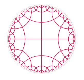
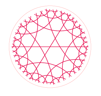
Example 2 –

Edge vectors and face vectors in general do not determine a vertex-transitive graph in a unique way. It is quite possible to obtain non-isomorphic graphs possessing the same edge and face vector. For example, consider the graphs on Figure 1. Both graphs correspond to the planar tiling of the hyperbolic plane with decagons; both are vertex-transitive and face-transitive graphs, and they have the same edge vectors. Nevertheless, the borders of the faces differ: for the graph on the left, it corresponds to $(\mathfrak{rgrbrbgbrb})$ and $(\mathfrak{rgbrb})^{2}$ on the right, where $\mathfrak{r}$, $\mathfrak{g}$ and $\mathfrak{b}$ respectively stand for the three different classes of edges.

Refer to captionRefer to captionRefer to captionRefer to caption
Figure 1: Non-isomorphic transitive graphs with the same edge and type vectors. The extremities of the lighter edge are non-isomorphic (see detail), which, considering the fact that both graphs are 3-connected, implies the non-isomorphism.


For an accurate description of the graph, some complementary informations are therefore needed. Following the intuitions in the case of TLF-planar Cayley graphs Ren (03), these informations are likely to come from local invariants linked to the classes of edges of $\Gamma$.

2.4 Edge neighborhoods

Let $e$ be an edge of $\Gamma$, and $T$ the finite tree composed of the edge $e$ and all edges incident to both extremities of $e$. An edge neighborhood for $e$ is a structure composed of the two edge vectors representing the classes of edges appearing around each extremity of $e$ in the same direction, where the first element of each vector corresponds to $e$, and two face vectors representing the classes of faces appearing around each

$\phi_{1}$ $\phi^{\prime}_{1}$1st extremity2nd extremity$e$

extremity, such that each corresponding edge and face vectors be locked together. Technically, we represent an edge neighborhood $\eta_{e}$ by the following structure:

$$\eta_{e}=\bigg{\{}\overbrace{\overbrace{\vphantom{\Big{\{}}[\xi_{1},\dots,\xi_{d}]}^{\textrm{Edge vector}},\overbrace{\vphantom{\Big{\{}}[\phi_{1},\dots,\phi_{d}]}^{\textrm{Face vector}}}^{\textrm{1st extremity}},\overbrace{\overbrace{\vphantom{\Big{\{}}[\xi^{\prime}_{1},\dots,\xi^{\prime}_{d}]}^{\textrm{Edge vector}},\overbrace{\vphantom{\Big{\{}}[\phi^{\prime}_{1},\dots\phi^{\prime}_{d}]}^{\textrm{Face vector}}}^{\textrm{2nd extremity}}\bigg{\}}$$
$$\textrm{for}~{}\{\xi_{i},\xi^{\prime}_{i}\}\subset\mathsf{E},\quad\textrm{and}~{}\{\phi_{i},\phi^{\prime}_{i}\}\subset\mathsf{F}$$

where $\xi_{1}=\xi^{\prime}_{1}=e$, $\phi_{1}=\phi^{\prime}_{d}$ and $\phi_{d}=\phi^{\prime}_{1}$. The vectors $[\xi_{1},\dots,\xi_{d}]$ and $[\phi_{1},\dots,\phi_{d}]$ are respectively the edge and face vectors of the first extremity, and the vectors $[\xi^{\prime}_{1},\dots,\xi^{\prime}_{d}]$ and $[\phi^{\prime}_{1},\dots\phi^{\prime}_{d}]$ correspond to the second extremity.

The color of an edge neighborhood corresponds to the class of edges of $e$. The separator of $\eta_{e}$, noted $\textsf{sep}(\eta_{e})$, correspond to the pair of classes of faces separated by $e$, here $(\phi_{1},\phi^{\prime}_{1})$. An edge neighborhood $\eta_{e}$ colored by $\mathfrak{e}$ is said to be coherent with a pair of vectors $(\xi,\phi)$ if and only if both edge vectors and face vectors at each extremity of $e$ are isomorphic to $(\xi,\phi)$.

Consider the set of edge neighborhoods of the same color of $\Gamma$. As for edge and face vectors, it is possible to define operations on this set:

  • Inversion and Symmetry: Inversion is the operation exchanging both extremities of the edge neighborhood, and corresponds to an exchange of the edge vectors and of the faces. Symmetry corresponds to the operation of symmetry (defined on the edge and face vectors) applied to each extremity of the edge neighborhood, while preserving the central edge.

  • Twist or Rearrangement of an extremity: Let $(\xi,\phi)$ be the edge and face vectors associated to one extremity of an edge neighborhood $\eta_{e}$. Any twist or rearrangement of $(\xi,\phi)$ that stabilizes the central edge leaves the faces separated by $\eta_{e}$ unchanged and extends naturally on the edge neighborhood.

Two edge neighborhoods $\eta_{1}$ and $\eta_{2}$ of the same color $\mathfrak{e}\in\mathsf{E}$ are said to be isomorphic if and only if it is possible to transform $\eta_{1}$ into $\eta_{2}$ by a sequence of inversions, symmetries, twists and rearrangements of any extremity. As was the case for the edge and face vectors, these operations describe all the possible edge neighborhoods in the embedding. We therefore select a single representative for each class of edges in $\Gamma$.

Lemma 10 (Edge neighborhood).

The edge neighborhood colored by $\mathfrak{e}\in\mathsf{E}$ of $\Gamma$ is independent of the choice of the embedding of $\Gamma$ and of the edge it is referring to, up to isomorphism.

Proof 4 –

The separator of a class of edge is independent of the edge (Lemma 8). Since finite faces are mapped onto finite faces by automorphisms of $\Gamma$, the $2$-connected components attached to the extremity of a class of edge are mapped onto $2$-connected components by automorphism. Therefore, the automorphisms mapping an edge onto another edge correspond to a rearrangement of composition of either natural transformations of the plane preserving this edge but exchanging its extremities (inversion and symmetry) or automorphisms leaving the edge and its extremities stable (rearrangements and twists). $\square$

Let $(\xi,\phi)$ be an edge and face vector. Two edges $e,f\in\xi$ labeled by the color $\mathfrak{e}\in\mathsf{E}$ are said to be equivalent, namely $e\sim f$, if and only if there exists an isomorphism of $(\xi,\phi)$ mapping $e$ onto $f$. Consider the set of edges in $\xi$ colored by $\mathfrak{e}$. Then $\textsf{eq}_{\xi,\phi}(\mathfrak{e})$ is the number of classes of equivalence inside this set with regard to $\sim$. The uniqueness of the edge neighborhood implies that $\textsf{eq}_{\xi,\phi}(\mathfrak{e})$ is at least one and at most two. As a matter of fact, each class of equivalence must correspond to an extremity of the edge neighborhood colored by $\mathfrak{e}$, and this neighborhood only has two extremities.

Example 3 –

Let us define edge neighborhoods coherent with the pair of edge and face vectors described in example 1. We represent the edge neighborhood associated to the edge colored by $\mathfrak{r}$ by the following picture:

           ${\color[rgb]{0,0,0}\gamma}$ ${\color[rgb]{0.7,0.7,0.7}\beta}$ ${\color[rgb]{0.5,0.5,0.5}\alpha}$ ${\color[rgb]{0.7,0.7,0.7}\beta}$ ${\color[rgb]{0,0,0}\beta}$ ${\color[rgb]{0.7,0.7,0.7}\beta}$ ${\color[rgb]{0,0,0}\gamma}$ ${\color[rgb]{0.5,0.5,0.5}\alpha}$ $2$ $3$ $4$ $5$ $5$ $4$ $3$ $2$1st extremity2nd extremity 1st extremity  : $[\mathfrak{r},\mathfrak{g},\mathfrak{b},\mathfrak{r},\mathfrak{r}]$  , $[\beta,\alpha,\gamma,\beta,\gamma]$ 2nd extremity  : $[\mathfrak{r},\mathfrak{b},\mathfrak{g},\mathfrak{r},\mathfrak{r}]$  , $[\gamma,\alpha,\beta,\gamma,\beta]$  

The fact that the faces colored by $\beta$ are infinite allows for the transformation of this labeling scheme by twists of either extremity.  

Example 4 –

While it could seem that the face vector is superfluous, i.e. that the graph could be described simply by its edge neighborhoods without any face vector, consider the particular case of graphs that are both vertex-transitive and edge-transitive, as in the Figure 2. The $[5;5;5;5]$ and $[3;7;3;7]$ graphs – denoted by their type vector – both belong to this class. Both possess the same edge neighborhoods and edge vectors. Yet these two graphs are obviously not isomorphic and their group of automorphisms are distinct, because the first is face-transitive, and the second possesses two different classes of faces.

Refer to caption Refer to caption
Figure 2: Non-isomorphic transitive graphs with the same edge neighborhoods, assuming that we remove the face vectors from the edge neighborhoods.


Whitney’s Theorem Whi (32) states that the finite planar 3-connected graphs have a unique embedding property i.e. their dual is uniquely defined. This property was extended to infinite graphs by Imrich Imr (75). As a matter of face, when $\Gamma$ is $3$-connected (while remaining transitive and TLF-planar), all faces of the graph are finite, and the graph is obviously composed of a unique $2$-connected component. Therefore the classes of isomorphisms of the geometrical invariants described in this section contain neither twists nor rearrangements. This is coherent with the unique embedding property. Notice that this property holds when $\Gamma$ is at least $2$-connected, in the case of transitive TLF-planar graphs. On the other hand, when $\Gamma$ is $1$-separable, these invariants provide an accurate description of the possible embeddings of the graph in the plane.

3 Labeling schemes

Our purpose in this section is to consider the geometrical invariants of $\Gamma$ and to prove that they are sufficient to give an exact description of the graph. The resulting description of the graph is called a labeling scheme, and extends the notion of labeling scheme for Cayley graphs, detailed in Cha (95); Ren (03).

3.1 Border automaton

Let $\mathsf{E}$ and $\mathsf{F}$ be two non-intersecting finite sets of colors. A labeling scheme of degree $d$ is a 3-tuple $(\xi,\phi,\eta)$ possessing the following properties:

  1. (i)

    $\xi\in\mathsf{E}^{d}$ is an edge vector and $\phi\in\mathsf{F}^{d}$ is a face vector;

  2. (ii)

    for each color $\mathfrak{e}\in\mathsf{E}$, $\textsf{eq}_{\xi,\phi}(\mathfrak{e})$ does not exceed two;

  3. (iii)

    for each color $\mathfrak{e}$ in $\xi$, there exists a unique edge neighborhood $\eta_{\mathfrak{e}}\in\eta$ of the same color; all edge neighborhoods in $\eta$ must be coherent with $(\xi,\phi)$ and if $\textsf{eq}_{\xi,\phi}(\mathfrak{e})=2$, then each class of equivalence must appear on an extremity of $\eta_{\mathfrak{e}}$.

Given a graph $\Gamma$, then $\xi$ and $\phi$ stand for $\Gamma$’s edge and face vectors, locked together. The set $\eta$ stands for the set of edge neighborhoods of $\Gamma$. In the following, $\eta_{\mathfrak{e}}$ stands for the edge neighborhood in $\eta$ colored by $\mathfrak{e}$. The isomorphisms of labeling schemes are defined as the isomorphisms of the elements of the scheme. The results in the previous sections ensure that for any pair $(\Gamma,G)$, there exists a labeling scheme $(\xi,\phi,\eta)$ corresponding to the coloring of the vertices and faces associated to the group $G$ of the graph $\Gamma$, up to isomorphism. Notice that the condition $(ii)$, along with Lemma 10 constrain the number of possible labeling schemes.

Consider a labeling scheme $(\xi,\phi,\eta)$. Let $e$ be an element of $\xi$ and $\eta_{e}\in\eta$ be the edge neighborhood labeled by the color of $e$. The operation of gluing $\eta_{e}$ with $e$ is possible if and only if there exists an edge neighborhood $\kappa$ isomorphic to $\eta_{e}$ such that one extremity of $\kappa$ be exactly equal to the pair $(\xi,\phi)$, with $e\in\xi$ as the central edge of the neighborhood $\kappa$.

Lemma 11 (Edge reconstruction).

Let $(\xi,\phi,\eta)$ be a labeling scheme, $e\in\xi$ and $\eta_{e}\in\eta$ colored by $e$, there exists a unique way to glue $\eta_{e}$ with $e$, up to isomorphism of the other extremity of $\eta_{e}$.

Proof 5 –

Suppose that there exists two different ways to glue $\eta_{e}$ onto $e$. If each extremity of $\eta_{e}$ may be glued onto $e$, this means that all edges colored by $e$ are equivalent with regard to $\sim$. If only one extremity of $\eta_{e}$ may be glued onto $e$, then there exists two classes of equivalence with regard to $\sim$ for the color of $e$, each of them at one extremity of $\eta_{e}$. In any case, since the number of classes of equivalence for the color of $e$ does not exceed two, that leads to a unique possibility to glue $\eta_{e}$ onto $e$, up to isomorphism. The existence follows from the fact that every class of equivalence of every color appears on an extremity of the associated edge neighborhood. $\square$

The gluing of edge neighborhoods allows the reconstruction of the graph. Let us start from an initial graph $\Lambda$ composed of all edges incident to a central vertex $v$. Suppose that these edges are labeled accordingly to the edge vector $\xi$. Obviously, this planar graph does not include faces for the moment, nevertheless we are expecting to build a face $\phi_{i}$ between the edges $\xi_{i}$ and $\xi_{i+1}$. By gluing the appropriate edge neighborhood $\eta_{\mathfrak{e}}$ onto the edge $\xi_{i}$, we create $d-1$ new edges incident to the other extremity of $\xi_{i}$ labeled such that the obtained edge neighborhood is isomorphic to $\eta_{\mathfrak{e}}$. The other extremities of these new edges correspond to new vertices of the graph. We will see later how it is possible to close the border of the faces.

Example 5 –

Consider the labeling scheme defined in Figure 3, where the set of colors are $\mathsf{E}=\{\mathfrak{b},\mathfrak{r},\mathfrak{g}\}$ and $\mathsf{F}=\{\alpha,\beta,\gamma\}$. It is based on the examples 1 and 3. We associate to each color in $\mathsf{E}$ a unique edge neighborhood. The face $\beta$ is supposed to be infinite, thus allowing by a twist exchanging the faces colored by $\beta$ that $\textsf{eq}_{\xi,\psi}(\mathfrak{r})=2$.


 γ𝛾{\color[rgb]{0,0,0}\gamma}β𝛽{\color[rgb]{0.7,0.7,0.7}\beta}2ptA 2ptA2 2ptA3 2ptA4 2ptA5 0.2504

(a) Edge and Face vectors

  γ β41352413(r) γ α44551122(b) α β55112233(g) γ β41352413(r) γ α44551122(b) α β55112233(g)\begin{array}[]{ccc}{\begin{pspicture}(-31.298pt,-51.21494pt)(31.298pt,36.98856pt){\psset{fillstyle=solid,fillcolor=lightvio,linecolor=violet,linearc=2.84526pt}\pscustom{{\pspolygon(-2.84526pt,-5.69054pt)(-8.53581pt,-11.38109pt)(-14.22636pt,-11.38109pt)(-14.22636pt,11.38109pt)(-2.84526pt,11.38109pt)}}}\rput[c](-8.53581pt,0.0pt){${\color[rgb]{0,0,0}\gamma}$}{\psset{fillstyle=solid,fillcolor=lightora,linecolor=orange,linearc=2.84526pt}\pscustom{{\pspolygon(2.84526pt,-11.38109pt)(14.22636pt,-11.38109pt)(14.22636pt,11.38109pt)(8.53581pt,11.38109pt)(2.84526pt,5.69054pt)}}}\rput[c](8.53581pt,0.0pt){${\color[rgb]{0.7,0.7,0.7}\beta}$}{\cnode(0.0pt,-14.22636pt){2.0pt}{A}}{\cnode(0.0pt,14.22636pt){2.0pt}{B}}{\psset{linecolor=lightvio}\ncline{A}{B}}{\cnode(14.22636pt,-14.22636pt){1.0pt}{A4}}{\psset{linecolor=lightvio}\ncline{A}{A4}}{\cnode(5.69054pt,-27.0301pt){1.0pt}{A3}}{\psset{linecolor=lightvio}\ncline{A}{A3}}{\cnode(-5.69054pt,-27.0301pt){1.0pt}{A2}}{\psset{linecolor=notwhite}\ncline{A}{A2}}{\cnode(-14.22636pt,-14.22636pt){1.0pt}{A1}}{\psset{linecolor=black}\ncline{A}{A1}}{\cnode(14.22636pt,14.22636pt){1.0pt}{B1}}{\psset{linecolor=notwhite}\ncline{B}{B1}}{\cnode(5.69054pt,27.0301pt){1.0pt}{B2}}{\psset{linecolor=black}\ncline{B}{B2}}{\cnode(-5.69054pt,27.0301pt){1.0pt}{B3}}{\psset{linecolor=lightvio}\ncline{B}{B3}}{\cnode(-14.22636pt,14.22636pt){1.0pt}{B4}}{\psset{linecolor=lightvio}\ncline{B}{B4}}{\psarc{->}(0.0pt,-14.22636pt){5.69054pt}{90.0}{0.0}}{\psarc{->}(0.0pt,14.22636pt){5.69054pt}{270.0}{180.0}}\rput(18.49428pt,14.22636pt){\tiny$4$}\rput(18.49428pt,-14.22636pt){\tiny$1$}\rput(8.53581pt,29.87537pt){\tiny$3$}\rput(8.53581pt,-29.87537pt){\tiny$5$}\rput(-8.53581pt,29.87537pt){\tiny$2$}\rput(-8.53581pt,-29.87537pt){\tiny$4$}\rput(-18.49428pt,14.22636pt){\tiny$1$}\rput(-18.49428pt,-14.22636pt){\tiny$3$}\rput(0.0pt,-42.67911pt){$(\mathfrak{r})$}\end{pspicture}}&{\begin{pspicture}(-31.298pt,-51.21494pt)(31.298pt,36.98856pt){\psset{fillstyle=solid,fillcolor=lightvio,linecolor=violet,linearc=2.84526pt}\pscustom{{\pspolygon(-2.84526pt,-5.69054pt)(-8.53581pt,-11.38109pt)(-14.22636pt,-11.38109pt)(-14.22636pt,11.38109pt)(-2.84526pt,11.38109pt)}}}\rput[c](-8.53581pt,0.0pt){${\color[rgb]{0,0,0}\gamma}$}{\psset{fillstyle=solid,fillcolor=lightgreen,linecolor=green,linearc=2.84526pt}\pscustom{{\pspolygon(2.84526pt,-11.38109pt)(14.22636pt,-11.38109pt)(14.22636pt,11.38109pt)(8.53581pt,11.38109pt)(2.84526pt,5.69054pt)}}}\rput[c](8.53581pt,0.0pt){${\color[rgb]{0.5,0.5,0.5}\alpha}$}{\cnode(0.0pt,-14.22636pt){2.0pt}{A}}{\cnode(0.0pt,14.22636pt){2.0pt}{B}}{\psset{linecolor=black}\ncline{A}{B}}{\cnode(14.22636pt,-14.22636pt){1.0pt}{A4}}{\psset{linecolor=notwhite}\ncline{A}{A4}}{\cnode(5.69054pt,-27.0301pt){1.0pt}{A3}}{\psset{linecolor=lightvio}\ncline{A}{A3}}{\cnode(-5.69054pt,-27.0301pt){1.0pt}{A2}}{\psset{linecolor=lightvio}\ncline{A}{A2}}{\cnode(-14.22636pt,-14.22636pt){1.0pt}{A1}}{\psset{linecolor=lightvio}\ncline{A}{A1}}{\cnode(14.22636pt,14.22636pt){1.0pt}{B1}}{\psset{linecolor=notwhite}\ncline{B}{B1}}{\cnode(5.69054pt,27.0301pt){1.0pt}{B2}}{\psset{linecolor=lightvio}\ncline{B}{B2}}{\cnode(-5.69054pt,27.0301pt){1.0pt}{B3}}{\psset{linecolor=lightvio}\ncline{B}{B3}}{\cnode(-14.22636pt,14.22636pt){1.0pt}{B4}}{\psset{linecolor=lightvio}\ncline{B}{B4}}{\psarc{->}(0.0pt,-14.22636pt){5.69054pt}{90.0}{0.0}}{\psarc{->}(0.0pt,14.22636pt){5.69054pt}{270.0}{180.0}}\rput(18.49428pt,14.22636pt){\tiny$4$}\rput(18.49428pt,-14.22636pt){\tiny$4$}\rput(8.53581pt,29.87537pt){\tiny$5$}\rput(8.53581pt,-29.87537pt){\tiny$5$}\rput(-8.53581pt,29.87537pt){\tiny$1$}\rput(-8.53581pt,-29.87537pt){\tiny$1$}\rput(-18.49428pt,14.22636pt){\tiny$2$}\rput(-18.49428pt,-14.22636pt){\tiny$2$}\rput(0.0pt,-42.67911pt){$(\mathfrak{b})$}\end{pspicture}}&{\begin{pspicture}(-31.298pt,-51.21494pt)(31.298pt,36.98856pt){\psset{fillstyle=solid,fillcolor=lightgreen,linecolor=green,linearc=2.84526pt}\pscustom{{\pspolygon(-2.84526pt,-5.69054pt)(-8.53581pt,-11.38109pt)(-14.22636pt,-11.38109pt)(-14.22636pt,11.38109pt)(-2.84526pt,11.38109pt)}}}\rput[c](-8.53581pt,0.0pt){${\color[rgb]{0.5,0.5,0.5}\alpha}$}{\psset{fillstyle=solid,fillcolor=lightora,linecolor=orange,linearc=2.84526pt}\pscustom{{\pspolygon(2.84526pt,-11.38109pt)(14.22636pt,-11.38109pt)(14.22636pt,11.38109pt)(8.53581pt,11.38109pt)(2.84526pt,5.69054pt)}}}\rput[c](8.53581pt,0.0pt){${\color[rgb]{0.7,0.7,0.7}\beta}$}{\cnode(0.0pt,-14.22636pt){2.0pt}{A}}{\cnode(0.0pt,14.22636pt){2.0pt}{B}}{\psset{linecolor=notwhite}\ncline{A}{B}}{\cnode(14.22636pt,-14.22636pt){1.0pt}{A4}}{\psset{linecolor=lightvio}\ncline{A}{A4}}{\cnode(5.69054pt,-27.0301pt){1.0pt}{A3}}{\psset{linecolor=lightvio}\ncline{A}{A3}}{\cnode(-5.69054pt,-27.0301pt){1.0pt}{A2}}{\psset{linecolor=lightvio}\ncline{A}{A2}}{\cnode(-14.22636pt,-14.22636pt){1.0pt}{A1}}{\psset{linecolor=black}\ncline{A}{A1}}{\cnode(14.22636pt,14.22636pt){1.0pt}{B1}}{\psset{linecolor=lightvio}\ncline{B}{B1}}{\cnode(5.69054pt,27.0301pt){1.0pt}{B2}}{\psset{linecolor=lightvio}\ncline{B}{B2}}{\cnode(-5.69054pt,27.0301pt){1.0pt}{B3}}{\psset{linecolor=lightvio}\ncline{B}{B3}}{\cnode(-14.22636pt,14.22636pt){1.0pt}{B4}}{\psset{linecolor=black}\ncline{B}{B4}}{\psarc{->}(0.0pt,-14.22636pt){5.69054pt}{90.0}{0.0}}{\psarc{->}(0.0pt,14.22636pt){5.69054pt}{270.0}{180.0}}\rput(18.49428pt,14.22636pt){\tiny$5$}\rput(18.49428pt,-14.22636pt){\tiny$5$}\rput(8.53581pt,29.87537pt){\tiny$1$}\rput(8.53581pt,-29.87537pt){\tiny$1$}\rput(-8.53581pt,29.87537pt){\tiny$2$}\rput(-8.53581pt,-29.87537pt){\tiny$2$}\rput(-18.49428pt,14.22636pt){\tiny$3$}\rput(-18.49428pt,-14.22636pt){\tiny$3$}\rput(0.0pt,-42.67911pt){$(\mathfrak{g})$}\end{pspicture}}\end{array}

(b) Edge neighborhoods
Figure 3: A labeling scheme of degree $5$ with its components.
${\color[rgb]{0.7,0.7,0.7}\beta}$2ptB1 $1$ $2$ $3$ $4$ $5$ $4$ $3$ $2$ $1$ $5$ $1$ $5$ $4$ $3$ $2$ $2$ $3$ $4$ $5$ $1$
Figure 4: Successive gluings of the edge neighborhoods along the border of the face colored by $\beta$.

Let us try to glue the edge neighborhoods consecutively, while following the edges constituting the border of the orange face (cf. Figure 4). We begin by gluing the golden edge neighborhood $\eta_{\mathfrak{g}}$ onto the unique golden $\mathfrak{g}$ edge belonging to the edge vector. Having glued two red edge neighborhoods $\eta_{\mathfrak{r}}$, we can ourselves continue the process indefinitely, by gluing red edge neighborhoods along the border of the face. If this labeling scheme corresponds to an existing graph $\Gamma$, then this process describes the border of a face colored by $\beta$ in $\Gamma$.  

Lemma 12 (Description of the faces).

Consider a graph $\Gamma$ and its labeling scheme $(\xi,\phi,\eta)$. It is possible to build a finite state automaton and an operation onto that automaton allowing to construct the borders of the faces of $\Gamma$.

Proof 6 –

Consider an automaton built over the alphabet $A$. A language $L\subset A^{\star}$ acts naturally over the set of states of the automaton. Therefore, we consider the following partition of the states of the automaton: two states $u$ and $v$ are equivalent if and only if there exists $l\in L$ such that it is possible to start from the state $u$, and reach the state $v$ by reading the word $l$ on the automaton. Now we will build an automaton by describing its set of states and the language acting on these states.

A configuration of a labeling scheme $(\xi,\phi,\eta)$ is a pair $(\mathcal{C},b)$ where $\mathcal{C}$ is a class of equivalence for $\sim$ in $(\xi,\phi)$ and $b\in\{+,-\}$ is a direction of rotation. A configuration represents a block of edges (separated by infinite faces) attached to a vertex, an edge inside this component and a direction expressing in which way the block is embedded in the plane. Two configurations are said to be equivalent if $(i)$ they correspond to two blocks, $(ii)$ it is possible to map the first block onto the second by an isomorphism of edge and face vectors and $(iii)$ this map sends the edge of the first configuration onto the edge of the second configuration, and maps the direction of rotation accordingly.

For a given labeling scheme, the number of configurations is finite, bounded by $2d$. These configurations define the states of our automaton. Let us define the following relations between configurations:

  • The next relation describes whether a configuration comes next to another one in the edge vector, given a direction of rotation: $(\mathcal{C},b)\overset{\textsf{\tiny next}}{\longrightarrow}(\mathcal{C}^{\prime},b)$ if and only if there exist $(\bar{\xi},\bar{\phi})$ isomorphic to $(\xi,\phi)$ such that if $\bar{\xi}_{i}$ (the $i^{\textrm{th}}$ element of the vector $\xi$) belongs to $\mathcal{C}$, the edge next to $\bar{\xi}_{i}$ according to the direction $b$ (if $b$ is positive, that is $\bar{\xi}_{i+1}$, otherwise that is $\bar{\xi}_{i-1}$) belongs to $\mathcal{C}^{\prime}$.

  • The inv relation describes how the configuration is modified when we cross the corresponding edge: $(\mathcal{C},b)\overset{\textsf{\tiny inv}}{\longrightarrow}(\mathcal{C}^{\prime},b^{\prime})$ if and only both configurations correspond to the same color of edge $\mathfrak{e}$ , and an edge neighborhood isomorphic to $\eta_{\mathfrak{e}}\in\eta$ has $(\mathcal{C},b)$ and $(\mathcal{C}^{\prime},b^{\prime})$ at its extremities.

Given these two relations, it is possible to build a finite state automaton on the set of configurations. This automaton is called the border automaton associated to this labeling scheme. By Lemma 11, it is connected. The inv relation is involutive, while the next relation may have more than one successor, therefore this automaton is non-deterministic in general. Determining the border of a face $\mathcal{F}$ is only a matter of reading the infinite word $(\textsf{next}\cdot\textsf{inv})^{\omega}$, with starting state a configuration such that the face $\mathcal{F}$ appears between this configuration and the configuration next to it in the automaton. Such a word is an orbit of the automaton under the action of $(\textsf{next}\cdot\textsf{inv})$. $\square$

For a given labeling scheme, we can associate to an element of the face vector – or a face – an orbit of the automaton. The colors of the faces are supposed to distinguish the classes of the faces under the group of automorphism. Two finite faces are said to be equivalent if they have the same orbit or orbits that correspond to the same border read in opposite directions. If two faces of the same color are not equivalent, then the labeling scheme is said to be invalid. Labeling schemes resulting from TLF-planar graphs are always valid. This property ensures that given two faces of the same color, there exists an automorphism mapping the first onto the second.

The orbits of the automaton can be classified into two categories : the cyclic orbits and the acyclic ones. Cyclic orbits correspond to faces that can be “closed”, meaning that their border is periodic. Consider the orbit containing the $i$-th edge of $\xi$, with positive direction of rotation. If this orbit is cyclic, then we define $k_{i}$ as the size of this orbit, otherwise $k_{i}=\infty$. Let $(a_{i}),i\in[1;d]$ be a set of formal letters such that $a_{i}=a_{j}$ if and only if the i-th and j-th face of $\phi$ are of the same color. The vector whose elements are the $k_{i}a_{i}$ (or simple $\infty$ if $k_{i}$ is infinite) is called the primitive type vector of $(\xi,\phi,\eta)$. A type vector $[l_{1},\dots,l_{d}]$ is said to be valid with regard to that labeling scheme if and only if there exists a valuation of the $(a_{i})$ in $\mathbb{N}$ such that $\forall i,l_{i}=k_{i}a_{i}$ and all values in the vector are greater than three.

3.2 Examples of construction

Example 6 –

Consider the labeling scheme defined in Figure 5, with degree $5$, $\textsf{E}=\{\mathfrak{b},\mathfrak{r},\mathfrak{g}\}$ and $\textsf{F}=\{\alpha,\beta,\gamma\}$. With each color in E we associate a unique edge neighborhood. Let us try to compute the associated border automaton. Even if $|\textsf{E}|=3$, there exist $10$ different configurations, one for each edge and direction of rotation. Since the next operation corresponds to a rotation of the edge vector, we represent the border automaton with two cycles of length $5$. On the Figure 6, next edges appear in black, while inv edges appear in dashed gray lines:

${\color[rgb]{0,0,1}\alpha}$ ${\color[rgb]{0.5,0.5,0.5}\beta}$2ptA 2ptA2 2ptA3 2ptA4 2ptA5 0.2504

β γ15243342(r) α β41551423(b) β β53122135(g) β γ15243342(r) α β41551423(b) β β53122135(g)\begin{array}[]{ccc}{\begin{pspicture}(-31.298pt,-51.21494pt)(34.14328pt,36.98856pt){\psset{fillstyle=solid,fillcolor=lightgreen,linecolor=green,linearc=2.84526pt}\pscustom{{\pspolygon(-2.84526pt,-5.69054pt)(-8.53581pt,-11.38109pt)(-14.22636pt,-11.38109pt)(-14.22636pt,11.38109pt)(-2.84526pt,11.38109pt)}}}\rput[c](-8.53581pt,0.0pt){${\color[rgb]{0.5,0.5,0.5}\beta}$}{\psset{fillstyle=solid,fillcolor=lightora,linecolor=orange,linearc=2.84526pt}\pscustom{{\pspolygon(2.84526pt,-11.38109pt)(14.22636pt,-11.38109pt)(14.22636pt,11.38109pt)(8.53581pt,11.38109pt)(2.84526pt,5.69054pt)}}}\rput[c](8.53581pt,0.0pt){${\color[rgb]{1,0,0}\gamma}$}{\cnode(0.0pt,-14.22636pt){2.0pt}{A}}{\cnode(0.0pt,14.22636pt){2.0pt}{B}}{\psset{linecolor=lightvio}\ncline{A}{B}}{\cnode(14.22636pt,-14.22636pt){1.0pt}{A4}}{\psset{linecolor=lightvio}\ncline{A}{A4}}{\cnode(5.69054pt,-27.0301pt){1.0pt}{A3}}{\psset{linecolor=notwhite}\ncline{A}{A3}}{\cnode(-5.69054pt,-27.0301pt){1.0pt}{A2}}{\psset{linecolor=black}\ncline{A}{A2}}{\cnode(-14.22636pt,-14.22636pt){1.0pt}{A1}}{\psset{linecolor=black}\ncline{A}{A1}}{\cnode(14.22636pt,14.22636pt){1.0pt}{B1}}{\psset{linecolor=lightvio}\ncline{B}{B1}}{\cnode(5.69054pt,27.0301pt){1.0pt}{B2}}{\psset{linecolor=black}\ncline{B}{B2}}{\cnode(-5.69054pt,27.0301pt){1.0pt}{B3}}{\psset{linecolor=black}\ncline{B}{B3}}{\cnode(-14.22636pt,14.22636pt){1.0pt}{B4}}{\psset{linecolor=notwhite}\ncline{B}{B4}}{\psarc{->}(0.0pt,-14.22636pt){5.69054pt}{90.0}{0.0}}{\psarc{->}(0.0pt,14.22636pt){5.69054pt}{270.0}{180.0}}\rput(18.49428pt,14.22636pt){\tiny$1$}\rput(18.49428pt,-14.22636pt){\tiny$5$}\rput(8.53581pt,29.87537pt){\tiny$2$}\rput(8.53581pt,-29.87537pt){\tiny$4$}\rput(-8.53581pt,29.87537pt){\tiny$3$}\rput(-8.53581pt,-29.87537pt){\tiny$3$}\rput(-18.49428pt,14.22636pt){\tiny$4$}\rput(-18.49428pt,-14.22636pt){\tiny$2$}\rput(0.0pt,-42.67911pt){$(\mathfrak{r})$}\end{pspicture}}&{\begin{pspicture}(-31.298pt,-51.21494pt)(34.14328pt,36.98856pt){\psset{fillstyle=solid,fillcolor=lightvio,linecolor=violet,linearc=2.84526pt}\pscustom{{\pspolygon(-2.84526pt,-5.69054pt)(-8.53581pt,-11.38109pt)(-14.22636pt,-11.38109pt)(-14.22636pt,11.38109pt)(-2.84526pt,11.38109pt)}}}\rput[c](-8.53581pt,0.0pt){${\color[rgb]{0,0,1}\alpha}$}{\psset{fillstyle=solid,fillcolor=lightgreen,linecolor=green,linearc=2.84526pt}\pscustom{{\pspolygon(2.84526pt,-11.38109pt)(14.22636pt,-11.38109pt)(14.22636pt,11.38109pt)(8.53581pt,11.38109pt)(2.84526pt,5.69054pt)}}}\rput[c](8.53581pt,0.0pt){${\color[rgb]{0.5,0.5,0.5}\beta}$}{\cnode(0.0pt,-14.22636pt){2.0pt}{A}}{\cnode(0.0pt,14.22636pt){2.0pt}{B}}{\psset{linecolor=black}\ncline{A}{B}}{\cnode(14.22636pt,-14.22636pt){1.0pt}{A4}}{\psset{linecolor=lightvio}\ncline{A}{A4}}{\cnode(5.69054pt,-27.0301pt){1.0pt}{A3}}{\psset{linecolor=lightvio}\ncline{A}{A3}}{\cnode(-5.69054pt,-27.0301pt){1.0pt}{A2}}{\psset{linecolor=notwhite}\ncline{A}{A2}}{\cnode(-14.22636pt,-14.22636pt){1.0pt}{A1}}{\psset{linecolor=black}\ncline{A}{A1}}{\cnode(14.22636pt,14.22636pt){1.0pt}{B1}}{\psset{linecolor=notwhite}\ncline{B}{B1}}{\cnode(5.69054pt,27.0301pt){1.0pt}{B2}}{\psset{linecolor=lightvio}\ncline{B}{B2}}{\cnode(-5.69054pt,27.0301pt){1.0pt}{B3}}{\psset{linecolor=lightvio}\ncline{B}{B3}}{\cnode(-14.22636pt,14.22636pt){1.0pt}{B4}}{\psset{linecolor=black}\ncline{B}{B4}}{\psarc{->}(0.0pt,-14.22636pt){5.69054pt}{90.0}{0.0}}{\psarc{->}(0.0pt,14.22636pt){5.69054pt}{270.0}{180.0}}\rput(18.49428pt,14.22636pt){\tiny$4$}\rput(18.49428pt,-14.22636pt){\tiny$1$}\rput(8.53581pt,29.87537pt){\tiny$5$}\rput(8.53581pt,-29.87537pt){\tiny$5$}\rput(-8.53581pt,29.87537pt){\tiny$1$}\rput(-8.53581pt,-29.87537pt){\tiny$4$}\rput(-18.49428pt,14.22636pt){\tiny$2$}\rput(-18.49428pt,-14.22636pt){\tiny$3$}\rput(0.0pt,-42.67911pt){$(\mathfrak{b})$}\end{pspicture}}&{\begin{pspicture}(-31.298pt,-51.21494pt)(34.14328pt,36.98856pt){\psset{fillstyle=solid,fillcolor=lightgreen,linecolor=green,linearc=2.84526pt}\pscustom{{\pspolygon(-2.84526pt,-5.69054pt)(-8.53581pt,-11.38109pt)(-14.22636pt,-11.38109pt)(-14.22636pt,11.38109pt)(-2.84526pt,11.38109pt)}}}\rput[c](-8.53581pt,0.0pt){${\color[rgb]{0.5,0.5,0.5}\beta}$}{\psset{fillstyle=solid,fillcolor=lightgreen,linecolor=green,linearc=2.84526pt}\pscustom{{\pspolygon(2.84526pt,-11.38109pt)(14.22636pt,-11.38109pt)(14.22636pt,11.38109pt)(8.53581pt,11.38109pt)(2.84526pt,5.69054pt)}}}\rput[c](8.53581pt,0.0pt){${\color[rgb]{0.5,0.5,0.5}\beta}$}{\cnode(0.0pt,-14.22636pt){2.0pt}{A}}{\cnode(0.0pt,14.22636pt){2.0pt}{B}}{\psset{linecolor=notwhite}\ncline{A}{B}}{\cnode(14.22636pt,-14.22636pt){1.0pt}{A4}}{\psset{linecolor=black}\ncline{A}{A4}}{\cnode(5.69054pt,-27.0301pt){1.0pt}{A3}}{\psset{linecolor=black}\ncline{A}{A3}}{\cnode(-5.69054pt,-27.0301pt){1.0pt}{A2}}{\psset{linecolor=lightvio}\ncline{A}{A2}}{\cnode(-14.22636pt,-14.22636pt){1.0pt}{A1}}{\psset{linecolor=lightvio}\ncline{A}{A1}}{\cnode(14.22636pt,14.22636pt){1.0pt}{B1}}{\psset{linecolor=lightvio}\ncline{B}{B1}}{\cnode(5.69054pt,27.0301pt){1.0pt}{B2}}{\psset{linecolor=lightvio}\ncline{B}{B2}}{\cnode(-5.69054pt,27.0301pt){1.0pt}{B3}}{\psset{linecolor=black}\ncline{B}{B3}}{\cnode(-14.22636pt,14.22636pt){1.0pt}{B4}}{\psset{linecolor=black}\ncline{B}{B4}}{\psarc{->}(0.0pt,-14.22636pt){5.69054pt}{90.0}{0.0}}{\psarc{->}(0.0pt,14.22636pt){5.69054pt}{270.0}{180.0}}\rput(18.49428pt,14.22636pt){\tiny$5$}\rput(18.49428pt,-14.22636pt){\tiny$3$}\rput(8.53581pt,29.87537pt){\tiny$1$}\rput(8.53581pt,-29.87537pt){\tiny$2$}\rput(-8.53581pt,29.87537pt){\tiny$2$}\rput(-8.53581pt,-29.87537pt){\tiny$1$}\rput(-18.49428pt,14.22636pt){\tiny$3$}\rput(-18.49428pt,-14.22636pt){\tiny$5$}\rput(0.0pt,-42.67911pt){$(\mathfrak{g})$}\end{pspicture}}\end{array}

Figure 5: Another labeling scheme of degree 5
0.1 2,1.8) $2$First orbit$3$Second orbit$2$Third orbitThe possible orbits are therefore $[1]$, $[2,4,5]$, and $[3]$. The first one corresponds to faces with red borders $\mathfrak{r}^{\star}$, and the third one to faces with blue borders $\mathfrak{b}^{\star}$. The others have border $(\mathfrak{bgr})^{\star}$. We have three possible classes of borders of the faces, corresponding to each orbit of the automaton and to each color in $\mathsf{F}$. The corresponding primitive type vector is: $[3n,m,3n,3n,p]$ for $(n,m,p)\in\mathbb{N}$. On Figure 7, there is an planar embedding in the hyperbolic plane of a graph possessing this labeling scheme and type vector $[3,4,3,3,5]$. The faces $\alpha$ correspond squares and the faces $\gamma$ to pentagons, while the faces with 3-colored borders are triangles. Notice that this graph possesses a trivial stabilizer and is therefore a Cayley graph.

  Figure 7: Example of a 3-connected TLF-planar vertex-transitive graph, with type vector $[5;3;4;3;3]$, associated to the labeling scheme described in the Example 4. Refer to caption  

 
Example 7 –

Consider now the case of example 5 page 5, where $\mathsf{E}=\{\mathfrak{b},\mathfrak{r},\mathfrak{g}\}$ and $\mathsf{F}=\{\alpha,\beta,\gamma\}$. As in the previous example, we associate to each color in $\mathsf{E}$ a unique edge neighborhood. The labeling scheme is valid with regard to our definitions. When we assume that the face $\beta$ is infinite, we come down with the border automaton appearing on Figure 8.

([angle=0.2,offset=0.4]A2)$1^{+}=5^{-}$ $2^{+}$ $3^{+}$ $4^{+}$ $4^{-}$ $3^{-}$ $2^{-}$
$3$First orbit$2$Second orbit$\infty$Third orbit
Figure 8: The border automaton associated to the labeling scheme in Figure 3.

The first orbit corresponds to the face $\gamma$, which is bordered by $(\mathfrak{rrb})^{\star}$. The second orbit corresponds to the face $\alpha$, bordered by $(\mathfrak{bg})^{\star}$. More interesting is the case of the face $\beta$. Notice that due to the possible twists, the next operator is not deterministic. This leads to faces bordered by aperiodic words from $\mathfrak{r}^{\omega}\mathfrak{gr}^{\omega}$. There does not exist any embedding of the graph can avoid these aperiodic faces (cf. Fig. 9), and all infinite faces either have a unique yellow edge in their border or none at all. The associated primitive type vector is given by $[\infty,3n,2m,\infty,3n]$ for values of $(m,n)\in\mathbb{N}$, which leads to 1-separable graphs such as the one on the right. For Cayley graphs, it is always possible to find an embedding where the border of the faces are periodic Ren (03). Hence, this set of graphs contains no Cayley graphs, because of this aperiodic border property.  

  Figure 9: Example of a 1-separable TLF-planar vertex-transitive graph, with type vector $[3;\infty;3;4;\infty]$, associated to the labeling scheme described in the Example 5. Refer to caption  

3.3 Realization

Every TLF-planar vertex-transitive graph possesses a valid labeling scheme and a vector type that is valid regarding to that scheme. Consider now the converse of this result: given a general valid labeling scheme, and a valid type vector, is it possible to produce a vertex-transitive graph that has the same labeling scheme and type vector ? Our goal in this section consists in building specific embeddings of vertex-transitive planar graphs with particular geometrical properties. Depending on the graph, we select an appropriate geometry: Euclidean, spherical or hyperbolic. As long as our graphs are TLF-planar, embeddings in spherical geometry will lead to finite graphs. Infinite faces thus can only occur in Euclidean and hyperbolic geometry. The following theorem constructs embeddings that are tilings of the plane by regular polygons.

Theorem 13 (Existence).

Given a labeling scheme $(\xi,\phi,\eta)$, and a valid type vector $[k_{1},\dots,k_{d}]$, there exists a TLF-planar vertex-transitive graph possessing this scheme and type vector. Moreover, all faces of the embedding are regular polygons.

Proof 7 –

Consider any point in the plane. We are going to evaluate the interior angle of a regular polygon of side length $l$, with $k_{i}$ sides, and then the total angle corresponding to all the polygons in the type vector must be equal to $2\pi$. The following values result from simple trigonometry in the different geometries:

$$\theta_{i}(l)=\left\{\begin{array}[]{cl}\textrm{Spherical :}&2\arcsin\left(\frac{\cos(\pi/k_{i})}{\cos(l/2)}\right)\\ \textrm{Euclidean :}&\frac{(k_{i}-2)}{k_{i}}\pi\\ \textrm{Hyperbolic :}&2\arcsin\left(\frac{\cos(\pi/k_{i})}{\cosh(l/2)}\right)\end{array}\right.\quad\textrm{and}\quad\sum_{i=1}^{d}\theta_{i}(l)=2\pi\quad(1)$$

The equation $(1)$ determines the choice of the geometry : let $\Sigma$ be the sum of the angles in the Euclidean plane. If $\Sigma=2\pi$, we choose the Euclidean geometry, and any value is possible for $l$ (the corresponding graphs will be homothetic). If $\Sigma<2\pi$, we choose the spherical geometry, whereas if $\Sigma>2\pi$ we select the hyperbolic geometry. In any case, there exists an unique solution of the equation $(1)$ that determines a unique value for the length $l$, and consequently for the angles $\theta_{i}$111Except for the following type vectors : $[3,3,p\geq 5]$, $[3,4,p\geq 6]$ and $[3,5,p\geq 9]$. There does not exist a labeling scheme validating any of these type vectors (cf p 15).. These values allow us to draw all the regular polygons that correspond to our type vector around a given point of the plane. Let $\epsilon$ be a point in the plane. By induction, we build a planar locally finite graph $\Gamma_{n}$, with a central vertex $\epsilon$, such that all vertices at distance $\leq n$ from $\epsilon$ have degree $d$. The graph $\Gamma_{1}$ is composed of the glued polygons of the first case, centered onto $\epsilon$, but restricted to the edges incident to $\epsilon$. The labeling of $\Gamma_{1}$ is chosen isomorphic to $(\xi,\phi)$, such that the face $\phi_{i}$ corresponds to a regular polygon with $k_{i}$ sides. Suppose now that we have built $\Gamma_{n}$. Consider the finite set of vertices of $\Gamma_{n}$ at distance $n$ of degree less than $d$. We shall build the remaining edges with geodesics, such that the length of the geodesic be $l$, and the angle at the vertex corresponding to the face $\phi_{i}$ be equal to $\theta_{i}(l)$. The labeling scheme describes how the edges must be labeled : take a vertex $s$ and an edge $e$ colored by $\mathfrak{e}$ incident to $s$. According to Lemma 11, there exists a unique way to glue the edge neighborhood $\eta_{\mathfrak{e}}$ onto $e$, up to isomorphism. The choice of the edge neighborhood is not crucial, because the isomorphisms leave the angles of the faces constant. The construction of $\Gamma_{n+1}$ is just a matter of gluing the edge neighborhoods on the edges possessing an extremity at distance $n+1$ from $\epsilon$, by choosing an adequate edge neighborhood isomorphic to $\eta_{\mathfrak{e}}$. This construction can not lead to intersecting edges. In fact; all edges have the same length, and inside a given face, all angles are the same. Therefore the construction of a face ultimately leads to a regular polygon in the plane. This answers the problem of the closure of the faces.

$\theta_{l}$ $\theta_{l}$ $\theta_{l}$ $\theta_{l}$ $\theta_{l}$ $\theta_{l}$ $l$ $l$ $l$ $l$ $l$ $l$ $l$?$\mathcal{F}$Length of the edges$l$Angle inside face $\mathcal{F}$ $\theta_{l}$

Hence the limit graph $\Gamma$ is well defined. This graph is vertex-transitive: the construction is independent of the starting vertex, and applying this construction with two different starting vertices creates an automorphism mapping the first vertex on the second. The labeling of the edges entails that the automorphism group is transitive. The automorphisms stabilizing a vertex exactly correspond to the classes of equivalence of the configurations. $\square$

Theorem 14 (Coherence).

If $\Gamma$ is a TLF-planar vertex-transitive graph that possesses a labeling scheme $(\xi,\phi,\eta)$ and a type vector $[k_{1},\dots,k_{d}]$, then the preceding construction yields a graph isomorphic to $\Gamma$.

Therefore, for any vertex-transitive graph obeying our conditions, it is possible to embed the graph in a particular geometry of the plane with regular polygons. Moreover, automorphisms of the graph map finite faces onto isometric faces. Consequently, in the case of the 2-connected graphs, every automorphism of $\Gamma$ extends into an isometry of the plane. This result appears in Babai Bab (97) in the case of 3-connected graphs, and is here extended to the larger case of the TLF-planar graphs. Notice that the case of $1$-separable graphs is more complex: even is the faces of the graph are regular polygons, example 7 shows that there exists graphs for which it is impossible to find an embedding where automorphisms may be realized by isometries of the plane. A direct consequence of this result pertains to the growth-rate of the TLF-planar graphs. When $\Gamma$ is $2$-separable, its structure is arborescent and its growth-rate is either linear or exponential. On the other hand, when $\Gamma$ is at least $3$-connected, the embedding of $\Gamma$ given by the Theorem 13 is quasi-isometric to the plane inside which it is defined. Therefore the growth-rate of the graph is either quadratic or exponential.

3.4 Combinatorial approach

Consider the problem of finding all the valid labeling schemes for graphs of degree $d$. The number of colors in E and F is bounded by $d$. Therefore the number of possible edge and face vectors is bounded by $d^{d-1}$, up to rotation, and the number of edge neighborhoods for a given color by $2d$. It is therefore possible to enumerate all possible labeling schemes, and then to extract the valid schemes by computing the border automaton. The particular properties of labeling schemes allow to drastically reduce this theoretical upper bound.
Theorem 15 (Enumeration).
Given a number d2𝑑2d\geq 2, it is possible to enumerate all TLF-planar transitive graphs having internal degree d𝑑d, along with their labeling scheme and primitive type vector.
A possible question lays in determining all possible type vectors for TLF-planar vertex-transitive graphs. We enumerate the graphs of a given degree, and eliminate the redundant ones by testing if they belong to the same class of isomorphism. For example, the possible type vectors for vertex-transitive graphs of degree 333 are: {[n,n,n],[n,2m,2m],[2n,2m,2p]}𝑛𝑛𝑛𝑛2𝑚2𝑚2𝑛2𝑚2𝑝\bigg{\{}[n,n,n],[n,2m,2m],[2n,2m,2p]\bigg{\}} …for values of n,m,p𝑛𝑚𝑝n,m,p such that the faces of the graphs are at least triangles. The set of planar graphs obtained is presented in appendix, and extends the vertex-transitive graphs presented in GS (87). Notice also that this set is strictly larger than the set of possible Cayley graphs of the same degree, containing in particular the graph associated to the dodecahedron, with type vector [5;5;5]555[5;5;5] and the icosidodecahedron, with type vector [3;5;3;5]3535[3;5;3;5], both of which are not Cayley graphs. More generally, this is the case of all tilings with type vector {[6n±1,6n±1,6n±1]}plus-or-minus6𝑛1plus-or-minus6𝑛1plus-or-minus6𝑛1\{[6n\pm 1,6n\pm 1,6n\pm 1]\}. This is an example o an infinite family of TLF-planar transitive graphs which are not Cayley. More precisely, for a given labeling scheme (ξ,ϕ,η)𝜉italic-ϕ𝜂(\xi,\phi,\eta) and valid type vector, we have the possibility to check whether the associated unlabeled graph is Cayley or not, by enumerating all Cayley graphs having the same type vector Ren (03), computing the labeling schemes of these transitive graphs and comparing them to (ξ,ϕ,η)𝜉italic-ϕ𝜂(\xi,\phi,\eta):
Corollary 16 (Cayley checking).
If ΓΓ\Gamma is a TLF-planar transitive graph, then it is decidable whether ΓΓ\Gamma is the Cayley graph of a group or not, and obtain an enumeration and a description of the groups having ΓΓ\Gamma as a Cayley graph.
Another side-result is the possibility to enumerate for a given graph ΓΓ\Gamma all the groups of automorphisms acting transitively on the set of vertices of ΓΓ\Gamma. This raises the question on finding graphs which are vertex-transitive but not Cayley, i.e. who do not possess a group of automorphism acting simply transitively on its vertices. Consider the stabilizer of a vertex of ΓΓ\Gamma: it must be a finite group of isometries of the plane fixing the vertex, hence it is either cyclic or dihedral. If this stabilizer does not contain any rotation, then the subgroup of direct isometries of Aut(Γ)AutΓ\textrm{Aut}(\Gamma) acts simply transitively on the vertices of ΓΓ\Gamma, therefore such graphs must possess rotations in their stabilizers. The multiply(k)multiply𝑘\textsf{multiply}(k) operation on a labeling scheme (ϕ,ξ,η)italic-ϕ𝜉𝜂(\phi,\xi,\eta) of degree d𝑑d consists in building another labeling scheme (ϕ,ξ,η)superscriptitalic-ϕsuperscript𝜉superscript𝜂(\phi^{\prime},\xi^{\prime},\eta^{\prime}) of degree k×d𝑘𝑑k\times d defined by: ϕsuperscriptitalic-ϕ\phi^{\prime} and ξsuperscript𝜉\xi^{\prime} consist of k𝑘k copies of ϕitalic-ϕ\phi and ξ𝜉\xi, i.e. ϕi=ϕ(i mod d)subscriptsuperscriptitalic-ϕ𝑖subscriptitalic-ϕ𝑖 mod 𝑑\phi^{\prime}_{i}=\phi_{(i\textrm{ \small mod }d)}, and ξi=ξ(i mod d)subscriptsuperscript𝜉𝑖subscript𝜉𝑖 mod 𝑑\xi^{\prime}_{i}=\xi_{(i\textrm{ \small mod }d)}; each edge neighborhood η𝔢subscriptsuperscript𝜂𝔢\eta^{\prime}_{\mathfrak{e}} is a copy of η𝔢subscript𝜂𝔢\eta_{\mathfrak{e}} where to the edge and face vectors at each extremity have been replaced by (ξ,ϕ)superscript𝜉superscriptitalic-ϕ(\xi^{\prime},\phi^{\prime}). The set of configurations of the automaton remains unchanged by this operation, as is the construction of the border automaton. This operation allows to build labeling schemes with stabilizers containing rotations. Moreover, this operation is invertible: for a labeling scheme whose stabilizer possesses rotations, it is possible to extract a labeling scheme without rotations by an operation of division.
Lemma 17 (Taxonomy of prime degree graphs).
Let $\Gamma$ be a 3-connected planar vertex-transitive graph of prime degree $d$. Either $\Gamma$ is a face and edge-transitive graph with type vector $[k;\dots;k]$, or it is a Cayley graph.
Proof 8 –
Consider the group of automorphisms of ΓΓ\Gamma and the stabilizer Gssubscript𝐺𝑠G_{s} of a vertex s𝑠s of ΓΓ\Gamma. Since the graph can be embedded in the plane by regular polygons, so that the automorphisms map the finite faces onto finite faces, G𝐺G is a group of isometries of the plane and Gssubscript𝐺𝑠G_{s} is a finite group of isometries of the plane leaving s𝑠s stable. If Gssubscript𝐺𝑠G_{s} contains a non-trivial rotation, since the degree of ΓΓ\Gamma is prime, the graph is edge and face-transitive. On the contrary, if Gssubscript𝐺𝑠G_{s} contains no rotation, then it has a single non-trivial element which is a symmetry. Then the subgroup of the direct isometries in G𝐺G acts simply and transitively on the vertices of ΓΓ\Gamma. Therefore ΓΓ\Gamma is a Cayley graph. \square
This analysis points out the classes of graphs that are likely not to be Cayley graphs. For the lesser degrees, these graphs are either face-transitive [k;;k]𝑘𝑘[k;\dots;k], or edge-transitive [k1,k2,,k1,k2]subscript𝑘1subscript𝑘2subscript𝑘1subscript𝑘2[k_{1},k_{2},\dots,k_{1},k_{2}]. There exists an example of graph of degree 999 belonging to this class that is neither face-transitive nor edge-transitive.

Discussion

The geometrical invariants of TLF-planar graphs allowed here the description of the graphs by their local properties, in the case of vertex-transitive graphs. Nevertheless, there exists different directions where we could extend this study. First, the dual graph of a transitive planar graph, is not transitive, but cofinite. That is to say that there exists only a finite number of orbits of the vertices under the action of the group of automorphisms. Even if these graphs in general do not respect the same geometrical properties as the transitive graphs, it would be interesting to study this family and their embeddings. We could then question the possibility of extending the representation by labeling schemes to cofinite graphs. Second, the key property of local finiteness is rather restrictive: our graphs possess one accumulation point at most. Yet Levinson showed that the number of accumulation points, if superior to one, is either two or infinite. The analysis of the embeddings of planar graphs with two or more accumulation points could lead to a geometrical representation for a larger class of vertex-transitive planar graphs.

References

  • Bab [97] László Babai. The growth rate of vertex-transitive planar graphs. In Proc. 8th Ann. Symp. on Discrete Algorithms, pages 564–573. New Orleans LA, ACM—SIAM, 1997.
  • Cha [95] T. Chaboud. Pavages et graphes de Cayley planaires. PhD thesis, Ecole Normale Supérieure de Lyon, Février 1995.
  • FI [79] H. Fleischner and W. Imrich. Transitive planar graphs. Mathematica Slovaca, 29(2):97–105, 1979.
  • Gar [95] Max Garzon. Models of massive parallelism: analysis of cellular automata and neural networks. Springer-Verlag, 1995.
  • GS [87] B. Grünbaum and G. C. Shephard. Tilings and patterns. W. H. Freeman Company, 1987.
  • HD [97] M.-C. Heydemann and B. Ducourthial. Graph symmetry: algebraic methods and applications, volume 497 of the NATO ASI Series (Series C: Mathematical and Physical Sciences), chapter Cayley graphs and Interconnection networks, pages 167–224. Kluwer Academic Publishers, 1997.
  • Imr [75] W. Imrich. On Whitney’s theorem on the unique embeddability of 3-connected planar graphs. In Recent advances in graph theory, Proc. Symp. Prague 1974, pages 303–306, 1975.
  • MD [98] J. Mazoyer and M. Delorme. Cellular automata : a parallel model, volume 460 of Mathematics and its applications. Kluwer, 1998.
  • MP [94] B. D. McKay and C. E. Praeger. Vertex-transitive graphs which are not Cayley graphs I. J. Austral. Math. Soc. (Series A), 56:53–63, 1994.
  • MP [96] B. D. McKay and C. E. Praeger. Vertex-transitive graphs that are not Cayley graphs II. J. Graph Theory, 22(4):321–334, 1996.
  • MR [90] B. D. McKay and J. F. Royle. The transitive graphs with at most 26 vertices. Ars Combin., 30:161–176, 1990.
  • Ren [03] D. Renault. Enumerating planar locally finite Cayley graphs. Submitted. Also available from arxiv.org, at ”http://arxiv.org/abs/cs.DM/0309017”, August 2003.
  • Roy [97] G. F. Royle. Catalogues of combinatorial objects. http://www.cs.uwa.edu.au/~gordon/data.html”, 1997. (Last access : ).
  • Whi [32] H. Whitney. Congruent graphs and the connectivity of graphs. American Journal of Math., 54:150–168, 1932.
  • Wol [84] J. Wolf. Spaces of constant curvature. Publish or Perish, Wilmington, 1984. Chap. 2.
Appendix

Appendix A Enumerations of vertex-transitive graphs

In the following sections, we enumerate all locally finite planar vertex-transitive graphs of small inner degree (from 3 to 4). Transitive graphs of degree $2$ correspond ot cyclic graphs. For the larger degrees, we enumerate all possible labeling schemes, each one corresponding to an enumerable family of planar vertex-transitive graphs. Some of these families may have the same representative in terms of unlabeled graphs, but the groups of automorphisms are distinct. These families are classified depending on whether their borders are periodic (P) or aperiodic (A). The following table displays the number of such classes : $$\begin{array}[]{|ccc||ccc||}\hline\cr\textrm{Degree}&\textrm{~{}~{}P~{}~{}}&\textrm{~{}~{}A~{}~{}}&\textrm{Degree}&\textrm{~{}~{}P~{}~{}}&\textrm{~{}~{}A~{}~{}}\\ \hline\cr 1&0&0&4&52&1\\ \hline\cr 2&1&0&5&174&>1\\ \hline\cr 3&16&0&6&775&>1\\ \hline\cr\end{array}$$ For each labeling scheme, we give the primitive type vector, and a description of the graph as a list containing the classes of edges and the border of the faces. Each class of edge is numbered $a_{i}^{k}$, where $k$ is a boolean indicating whether the associated edge neighborhood reverses the direction of rotation of the edge vector or not. Each border of the faces is a word on the edge classes corresponding to an orbit in the border automaton repeated a given number of times.

Figure 6: The border automaton associated to the labeling scheme in Figure 5.