On computing fixed points for generalized
sandpiles

Abstract

We prove fixed points results for sandpiles starting with arbitrary initial conditions. We give an effective algorithm for computing such fixed points, and we refine it in the particular case of SPM.

1 Introduction

Sandpiles are a simple but meaningful formal model for the simulation of systems governed by self-organized criticality (SOC). These systems, starting from any initial configuration, evolve to a “critical” state. Any perturbation of this critical state, no matter how small, originates a deep and uncontrollable reorganization of the whole. Then, they start evolving towards another critical state and so on. SOC systems are commonly used for simulating natural phenomena like snow avalanches, dune formations, but also woods fires and even, stock exchange crashes.

The first discrete model for sandpiles, (later on) called SPM (Sand Pile Model), has been introduced in [1]. It is based on a simple local rule: a sand grain falls on its right if the difference between its sandpile and the one on its right is bigger than a certain amount of grains. In [3, 2, 5, 6], the model has been mathematically formalized and studied as a discrete dynamical system. In particular, they proved that SPM has fixed point dynamics and exhibited formulas for the precise expression of fixed points and for computing the transient length.

Similar results exist for a more complete model, IPM$(k)$ (Ice Pile Model) introduced in [5]. The results found for these two models, synthesized in [4], are very interesting and complete but they concern only very special initial conditions in which all the sand grains are concentrated in a unique pile and there is no grain elsewhere.

In this paper we generalize those results to arbitrary initial conditions. Of course, due to much greater combinatorial complexity of the problem, we do not have nice formulas but we give a fast algorithm for computing the fixed point.

This paper is structured as follows. The next section recalls basic definitions about the main sandpile models. Section 3 resumes the main known results, which are generalized to arbitrary sandpiles in Section 4. Section 5 improves the results of the previous section for the special case of SPM. In the final section we draw our conclusion and give some perspectives.

2 Basic definitions

A sandpile is a finite sequence of integers $(a_{1},\ldots,a_{l})$; $l\in\mathbb{N}$ is the length of the pile. Sometimes a sandpile is also called a configuration. Given a sandpile $(a_{1},\ldots,a_{l})$, the integer $n=\sum_{i=1}^{l}a_{i}$ is the number of grains of the pile. Given a configuration $(a_{1},\ldots,a_{l})$, a subsequence $a_{i},\dots,a_{j}$ (with $1\leq i,j\leq l$ and $i<j$) is a plateau if $a_{k}=a_{k+1}$ for $i\leq k<j$; a subsequence $a_{i},a_{i+1}$ is a cliff if $a_{i}-a_{i+1}\geq 2$.

In the sequel, each sandpile $(a_{1},\ldots,a_{l})$ will be conveniently represented on a two dimensional grid where $a_{i}$ is the grain content of column $i$.

A sandpile system is a finite set of rules that tell how the sandpile is updated. SPM is the most known and the most simple sandpile system. It consists in just one local rule. Moreover, all initial configurations contain $n$ grains in the first column and nothing elsewhere i.e. they are of type $(n)$. The system rule can be defined in two equivalent ways. The former, introduced in [1], considers the sequence $z_{i}=a_{i}-a_{i+1}$ of differences between two consecutive columns $i$ and $i+1$. If $z_{i}\geq 2$, then a sand grain falls from column $i$ to $i+1$ giving the following new sequence of differences (see Figure 1(a)):

$$\left\{\begin{array}[]{rcl}z^{\prime}_{i-1}&=&z_{i-1}+1\\ z^{\prime}_{i}&=&z_{i}-2\\ z^{\prime}_{i+1}&=&z_{i+1}+1\enspace.\end{array}\right.$$

The latter, introduced in [2], deals with the real height of consecutive columns. It has the advantage of having a simple and intuitive graphical representation. The updating rule is defined as follows (see Figure 1(b))

$$\left\{\begin{array}[]{rcl}a^{\prime}_{i}&=&a_{i}-1\\ a^{\prime}_{i+1}&=&a_{i+1}+1\\ \end{array}\right.\qquad\textrm{if}\;a_{i}-a_{i+1}\geq 2\enspace.$$

(a) Height differences.

(b) Column grain content.

Figure 1: updating in the SPM model.

Remark that there are also two ways of evolving the sandpile system: parallel and sequential execution mode. In parallel mode, all applicable rules are applied at once; only one rule at a time is applied in the sequential mode. For example, in Figure 1, several grains might fall at the same time (columns $2$ and $4$ may lose a grain): the next configuration depends on the execution mode; if we choose the sequential mode, then the next configuration depends also on the column to which one applies the system rule. The execution mode is fixed from the beginning and does not change along the evolution of the system. In the sequel, we will be mainly interested in the sequential mode for the simplicity sake.

IPM$(k)$ is another usual model that extends SPM. It contains the vertical rule of SPM defined above, plus a horizontal rule: the grains can slide on a horizontal plateau of length at most $k$ as follows

$$(\ldots,p+1,\underbrace{p,p,\ldots,p}_{k^{\prime}\;\textrm{times}\;\,(k^{\prime}\leq k)},p-1,\ldots)\xrightarrow{\quad\textrm{IPM$(k)$}_{hor}\quad}(\ldots,p,p,p,\ldots,p,p,\ldots)\enspace.$$

This rule can be used to simulate slopes of less than 45°, while the vertical rule (when generalizing the definition of cliffs to any difference of height) simulates slopes bigger than 45°.

A sequence of configurations $\left\{c_{i}\right\}_{i\in\mathbb{N}}$ is called an orbit of initial condition $c_{1}$ if for all $i\in\mathbb{N}$, $c_{i+1}$ is obtained from $c_{i}$ via the application of a system rule. Remark that there might be more than one orbit for the same initial condition.

The set of orbits $O_{c}$ with the same initial condition $c$ is graphically represented by the orbit graph $\mathcal{G}_{c}=\left\langle V,E\right\rangle$, where $V$ is the set of all configurations belonging to orbits in $O_{c}$ and $(a,b)\in E$ ($E\subseteq V\times V$) if and only if $b$ is obtained from $a$ by an application of a system rule. Denote $\mathcal{G}_{c}^{l}$ the orbit graph of the configuration $c$ in which all configurations (including $c$) have length at most $l$. Given an orbit graph $\mathcal{G}=\left\langle V,E\right\rangle$ we say that a configuration $c$ belongs to $\mathcal{G}$, denoted $c\in\mathcal{G}$ if $c\in V$. A vertex $v\in V$ is a fixed point of a directed graph $G=\left\langle V,E\right\rangle$ if $v$ has no outgoing edges. Given two graphs $G_{1}=\left\langle V_{1},E_{1}\right\rangle$ and $G_{2}=\left\langle V_{2},E_{2}\right\rangle$, $G_{1}$ is a sub-graph of $G_{2}$ if $V_{1}\subseteq V_{2}$ and $E_{1}\subseteq E_{2}$.

As an example, Figure 2 shows the orbit for the initial configuration $(8)$ according to both sequential and parallel execution modes for SPM. One can remark that both sequential and parallel execution mode lead to the same fixed point $(3,2,2,1)$. The difference between the two evolutions seems to consist only in the transient length. These remarks are true and will be justified in the following section.

(a) Sequential execution mode.

(b) Parallel execution mode.

Figure 2: orbit of SPM for $n=8$ with respect to execution mode.

3 Known results

The results of this section are essentially taken from [2] and [5]. We stress that, for simplicity sake, only the sequential execution mode is considered.

3.1 Fixed points

First we recall the results for SPM, and for the slightly more complex model IPM$(k)$.

The following theorem shows that, for any initial configuration $(n)$, the orbit graph of SPM has a very special structure.

Theorem 1 ([2])

For any integer $n$, the orbit graph $\mathcal{G}_{(n)}$ for SPM is a lattice and is finite.

As a consequence of Theorem 1 we have that SPM has fixed point dynamics starting from any configuration $(n)$. Moreover, this fixed point is unique and it is reached regardless of the order in which transitions are made and regardless of the execution mode (parallel or sequential) that has been chosen. The following lemma characterizes the elements of the lattice.

Lemma 2 ([5])

Consider a configuration $c$ and let $n$ be its number of grains. Then, $c\in\mathcal{G}_{(n)}$ for SPM if and only if it is decreasing and between any two plateaus there is at least a cliff.

Remark 1

Consider a configuration $c$ and let $n$ be its number of grains. Assume that $c$ contains a plateau of length $3$. Such a plateau can be seen as two consecutive plateaus of length $2$. Thus, by Lemma 2, $c$ does not belong to $\mathcal{G}_{(n)}$.

The previous condition is not necessary for the characterization of the fixed point. Notwithstanding, it allows to obtain a much simpler proof of the following Theorem 3.

Notation.

A couple of integers $\left\langle p,k\right\rangle$ is the decomposition of $n\in\mathbb{N}$ in its integer sum if $n=k+\sum_{i=1}^{p}i=k+\frac{p\cdot(p+1)}{2}$.

Theorem 3 ([2])

There exists a unique decomposition of $n\in\mathbb{N}$ in its integer sum. Then, the fixed point $\Pi$ obtained starting from the initial configuration $(n)$ is the following

$$\Pi=\left\{\begin{array}[]{l@{\hspace{1cm}}l}(p,p-1,\ldots,1)\hfil\hskip 28.45274pt&\textrm{if}\;k=0\\ (p,p-1,\ldots,k+1,k,k,k-1,\ldots,1)\hfil\hskip 28.45274pt&\textrm{otherwise}\enspace.\end{array}\right.$$

Similar results hold for IPM$(k)$, we recall the main ones here. They can be found in their original form in [5].

Theorem 4 ([5])

For any integer $n$, the orbit graph $\mathcal{G}_{(n)}$ for IPM$(k)$ is a lattice and is finite.

Again, there exist a characterization of the configurations of the lattice [5]. It is a generalization of Lemma 2 which will not be used explicitly here. Remark that this allows to give the exact form of the fixed point of a configuration for IPM$(k)$.

3.2 Transient length

We have seen that according to the usual models, the sandpile $(n)$ evolves to a fixed point. It can be interesting to know how much time (i.e. how many iterations of the system rule) it takes to reach such a fixed point - of course this time depends on the execution mode.

For SPM, in the sequential execution mode, it is easy to compute the number of steps needed to reach the fixed point: it suffices to remark that the grains in the $i$-th column took $i$ iterations to reach it; taking the sum all over the number of grains of the fixed point one finds the number of iterations.

Theorem 5 ([2])

The length of the transient to reach the fixed point starting from the initial configuration $(n)$ for SPM is given by the following formula

$$t_{seq}=\frac{1}{6}(p+1)p(p-1)+\frac{1}{2}k(2p+1-k)=\mathcal{O}(n^{3/2})\enspace,$$

where $\left\langle p,k\right\rangle$ is the decomposition of $n$ in its integer sum.

When parallel execution mode is used for SPM, things are a little bit more complex and one can only give an upper and a lower bound for the transient length.

Theorem 6 ([2])

In the parallel execution mode, the length of the transient to reach the fixed point starting from the initial configuration $(n)$ for SPM can be bounded as follows

$$\mathcal{O}(n)=\frac{t_{seq}}{p-1}\leq t_{par}\leq t_{seq}=\mathcal{O}(n^{3/2})\enspace,$$

where $\left\langle p,k\right\rangle$ is the decomposition of $n$ in its integer sum.

Finally for IPM$(k)$, all the paths from $(n)$ to the fixed point do not necessarily have the same length, but the longest chain in sequential mode is known. Its exact expression can be found in [5].

4 Generalization to arbitrary sandpiles

The results from the previous section are very complete, but they only apply to the particular case of initial configurations of length one.

A little more general study was started in [2], where the authors remarked that when starting from decreasing configurations (for all $0\leq i<l$, $a_{i}\geq a_{i+1}$) the lattice structure is maintained with SPM. This result is extended in [6], where the author exhibits the set of fixed points but she does not associate to each initial configuration the corresponding fixed point.

In this paper, we try to generalize these results to arbitrary initial configurations giving a fast algorithm for computing fixed points.

Description of the algorithm. It consists in the iteration of two major steps:

Cut:

the configuration is divided into intervals so that the formulas of the next step can be applied;

Compute:

each interval is analyzed trying to figure out how it will be within a few iterations steps of the model.

Remark that it is necessary to iterate since some grains can pass from one interval to another. Consider the case of two isolated columns of grains $(m,0,\ldots,0,n)$. The first column will collapse. Then, depending on the model chosen and on the value of $m$, $n$ and of the gap between the two columns, the grains of the first column will be blocked by the second one or they will partially cover it.

From now on, to simplify notations and proofs the results will be given only for SPM. Their extension to other models such as IPM$(k)$ is straightforward, using the formulas given in [5]. In fact our results extend to all models satisfying two conditions: lattice structure of the orbit graph, and reachability detection (one must be able to say whether a given configuration is reachable or not, in a way similar to Lemma 2). Hence we will implicitly consider this class of sandpile models in the sequel of the paper when talking about “all” models. Next section justifies the restriction to these models.

4.1 Cut

The way we are going to split the configuration into intervals is very simple: each interval has to contain a configuration which is reachable by the model, and it is the longest satisfying this property.

At that point, the previous results need to be extended. Indeed, their authors supposed that the grains could move as far as possible. In the present case, the movement is limited to fixed intervals, grains are prevented from going too far on the right. All the results remain true, but have to be reformulated.

Lemma 7

For all initial configurations $c$ for SPM, $\mathcal{G}_{c}$ has no cycles.

Proof.  Given a configuration $c=(a_{1},\ldots,a_{l})$, consider the quantity $\varphi(c)=\sum_{i=1}^{l}\sum_{j=1}^{a_{i}}j$. If $c^{\prime}=(a^{\prime}_{1},\ldots,a^{\prime}_{l^{\prime}})$ is obtained from $c$ by applying the SPM rule at column $i\leq l$, then $\varphi(c^{\prime})=\varphi(c)-a_{i}+a^{\prime}_{i+1}=\varphi(c)-a_{i}+a_{i+1}+1$. Since the rule could be applied, $a_{i}\geq a_{i+1}+2$, which implies $\varphi(c^{\prime})<\varphi(c)$; in other words, the SPM system rule is irreversible. ❏

Our algorithm will only work with models having this irreversibility property. IPM$(k)$ has it, and any realistic model should have it.

Lemma 8

For all initial configurations $c$ of length at most $l$ for SPM, $\mathcal{G}_{c}^{l}$ has a unique fixed point $\Pi$. Moreover, $\Pi\in\mathcal{G}_{c}$.

Proof.  Let $c$ be a configuration of length at most $l$, with $n$ grains. First of all remark that $\mathcal{G}_{c}^{l}$ is a sub-graph of $\mathcal{G}_{c}$ since for every configuration in $\mathcal{G}_{c}^{l}$, the path from the root $(n)$ to this configuration is also in $\mathcal{G}_{c}$ (it just consists in applying system rules to columns of index less than $l$).

Hence $\mathcal{G}_{c}^{l}$ is finite, and by Lemma 7, it has no cycles. Therefore every path starting from a configuration $c$ reaches a fixed point. Assume that $\Pi_{1}$ and $\Pi_{2}$ are two distinct fixed points of $\mathcal{G}_{c}^{l}$. They also belong to $\mathcal{G}_{c}$, so they satisfy Lemma 2 i.e. they are decreasing and contain at most one plateau (as they are fixed points of SPM, there are no cliffs). Their structure is represented on Figure 3. They are simply “staircases” with the addition of $k$ grains:

$$\Pi_{j}=\left\{\begin{array}[]{l@{\hspace{2mm}}l}(p_{j},p_{j}-1,\ldots,p_{j}-l+1)\hfil\hskip 5.69054pt&\textrm{if $k_{j}=0$}\\ (p_{j},p_{j}-1,\ldots,p_{j}-\alpha_{j},p_{j}-\alpha_{j},\ldots,p_{j}-l+2)\hfil\hskip 5.69054pt&\textrm{otherwise},\end{array}\right.$$

with $\alpha_{j}=l-k_{j}-1$.

Figure 3: structure of a fixed point in $\mathcal{G}_{c}^{l}$. The symbol $q$ will be defined in Section 4.2.

Counting the number of grains in $\Pi_{1}$ and $\Pi_{2}$ gives

$$\begin{array}[]{rcl}n&=&\displaystyle\sum_{i=1}^{l}(p_{1}+1-i)+k_{1}=\displaystyle\sum_{i=1}^{l}(p_{2}+1-i)+k_{2}\qquad(0\leq k_{1},k_{2}<l)\\[2.15277pt] &=&\dfrac{1}{2}l(2p_{1}+1-l)+k_{1}=\dfrac{1}{2}l(2p_{2}+1-l)+k_{2}\enspace.\end{array}$$ (1)

This implies that $|p_{2}-p_{1}|=\frac{1}{l}\cdot|k_{2}-k_{1}|<1,$ and as $p_{1}$ and $p_{2}$ are integers we have $p_{1}=p_{2}$. It follows that $k_{1}=k_{2}$, and $\Pi_{1}=\Pi_{2}$. ❏

The irreversibility condition needed to apply the algorithm to a particular model can be relaxed. In fact, what is needed for the previous lemma to work is a lattice structure. This ensures irreversibility and unicity of the fixed point.

Proposition 9

For all initial configurations $c$ of length at most $l$ for SPM, $\mathcal{G}_{c}^{l}$ is a lattice and $\mathcal{G}_{c}^{l}\subseteq\mathcal{G}_{c}$.

Proof.  In the proof of Lemma 8, we saw that $\mathcal{G}_{c}^{l}$ is a sub-graph of $\mathcal{G}_{c}$. By Lemma 7 and 8 we have the thesis. ❏

Lemma 10

Consider the SPM model, a configuration $c$ of length at most $l$ and let $n$ be its number of grains. Then, $c\in\mathcal{G}_{(n)}^{l}$ if and only if it is decreasing and between any two plateaus there is at least a cliff.

Proof.  Consider a configuration $c\in\mathcal{G}_{(n)}^{l}$, where $n$ is the number of grains of $c$. By Proposition 9, $c$ belongs also to $\mathcal{G}_{(n)}$ and hence it satisfies the hypothesis of Lemma 2.

For the opposite implication, let $c=(a_{1},\ldots,a_{k})$ be a decreasing configuration of length at most $l$ in which any two plateaus have a cliff in between. Let $n$ be the number of grain of $c$. By Lemma 2, $c$ belongs to $\mathcal{G}_{(n)}$. If we consider the path going up to the root, all the configurations encountered are of length less than $l$ since the application of the system rule can only increase the length of a configuration. All the applications of the system rule take place in the interval $[1,l-1]$, hence each element of the path is also in $\mathcal{G}_{(n)}^{l}$. ❏

The previous lemma underlines the second condition that is needed for the sandpile model used in the algorithm: it should be possible to detect whether a configuration is reachable by the model. Moreover, for complexity issues (see Section 4.4), it should be as fast as possible (for SPM and IPM$(k)$, it is linear, as a single scan suffices).

Using the previous lemma one can complete the characterization of $\mathcal{G}^{l}$ that begun with Proposition 9.

Proposition 11

For any integer $n$ it holds that

$$\mathcal{G}_{(n)}^{l}=\mathcal{G}_{(n)}\big{[}\{c\in\mathbb{N}^{l}\}\big{]}\enspace,$$

where for any graph $G=\left\langle V,E\right\rangle$, $G[V^{\prime}]$ is the sub-graph generated by the set of vertices $V^{\prime}\subseteq V$.

The previous proposition means that for SPM, $\mathcal{G}_{(n)}^{l}$ is exactly the sub-graph of $\mathcal{G}_{(n)}$ restricted to the configurations of length at most $l$, keeping all edges between these configurations. By Proposition 9, this sub-graph is also a lattice. This holds for any model having the lattice structure and the reachability detection, this is the case for example for IPM$(k)$.

The cut step is performed using Lemma 2, Propositions 9 and 11. A scan is performed in order to find the maximal intervals in which the corresponding sub-configurations are in $\mathcal{G}_{c}$. For example, for SPM, a new interval starts whenever there are two consecutive columns $i$ and $i+1$ such that $a_{i}<a_{i+1}$, or there is a second plateau not separated by a cliff (see Listing 1).

⬇

procedure cut (c[]) { // c is the initial configuration

nbp = 0; // number of plateaus

I = $\emptyset$; // set of right extremities of the intervals

for (i=1; i<l; i++) {

if (c[i+1] > c[i]) { // increase

I = I $\cup\;\;\{$i$\}$;

nbp = 0;

} else if (c[i] - c[i+1] >= 2) { // cliff

nbp = 0;

} else if (c[i+1] == c[i]) { // plateau

nbp ++;

if (nbp == 2) {

I = I $\cup\;\;\{$i$\}$;

nbp = 0;

}

}

}

return I;

}

Listing 1: procedure for cutting a configuration into intervals using SPM.

By Lemma 2, the sub-configurations given by the intervals are in $\mathcal{G}_{c}$ and they are “maximal”. Moreover, by Propositions 9 and 11, we know that each sub-configuration is in $\mathcal{G}_{(n_{i})}^{l_{i}}$ and that it reaches the fixed point of $\mathcal{G}_{(n_{i})}^{l_{i}}$, where

• $c_{i}$ is the configuration corresponding to the $i^{\textrm{\scriptsize th}}$ interval, $c_{i}=(a_{k})_{k\in I_{i}}$ ;

• $l_{i}=|I_{i}|$ is the length of $c_{i}$ ;

• $n_{i}$ is the number of grains of $c_{i}$ .

Remark that the quantities $l_{i}$ and $n_{i}$ can be computed inside the procedure cut.

The last interval – reached when the scanning procedure arrives at $a_{l}$ – is a “special case”: it is treated exactly like in the usual model, supposing there is as much space as necessary. An example of “cut” for the SPM model is shown in Figure 4.

Figure 4: example of intervals after the cut step, for SPM.

4.2 Compute

In this section we show formulas for finding the fixed point locally to each interval. From now on and only for this section, we consider a generic interval and hence the index $i$ will be omitted in the notations. Again, only SPM will be considered to simplify the formulas, but similar results hold for other models.

The structure of the global configuration after the cut has to be precisely determined: we shall find the fixed point of every configuration in each interval.

In the proof of Lemma 8, we saw that the fixed point $\Pi$ of an interval with SPM is a kind of “staircase” as depicted in Figure 3. We need the expression of $p$ (height of the leftmost column of the fixed point), $q$ (height of the rightmost column) and $k$ (number of exceeding grains) in terms of $n$ and $l$.

Equation (1) implies that

$$p=\left\lfloor\frac{n}{l}+\frac{l}{2}-\frac{1}{2}\right\rfloor\enspace.$$

Then, $k=n-\frac{1}{2}l(2p+1-l)\enspace.$ For $q$, the same calculation is done, counting the number of grains in the fixed point

$$\begin{array}[]{rcl}n&=&\displaystyle\sum_{i=1}^{l}(q+l-i)-k^{\prime}\qquad(k^{\prime}=l-k\mod l,\quad\textrm{hence }0\leq k^{\prime}<l)\end{array}$$

one finds $q=\left\lceil\dfrac{n}{l}-\dfrac{l}{2}+\dfrac{1}{2}\right\rceil$.

Remark 2

The quantity $k$ is not necessarily a real number of grains. Indeed, when the fixed point finishes by $(\ldots,2,1,0,0)$, we have $k=1$. This does not correspond to a grain, but compensates a negative grain introduced when computing $p$ (the last term of the sum equals $-1$).

Moreover, the last interval has to be treated in another way, as it has infinite length. Choosing $l=\left\lceil\frac{\sqrt{8n+1}-1}{2}\right\rceil$, value obtained from the results in [2], would solve the problem. It corresponds to the length of the fixed point obtained from the configuration $(n)$. With this new value, the calculation of $p$ and $q$ is correct.

4.3 Correctness

In this section we will prove that the algorithm finishes and gives the correct fixed point. All results are stated for all suitable models. Proofs are given for the SPM case only, for simplicity sake.

The superscript ^f for the quantities $I_{i},c_{i},n_{i}$ mean that we use their value they have at the end of the algorithm.

Proposition 12

For any configuration, the algorithm finishes and returns a fixed point.

Proof.  Because of the irreversibility (Lemma 7) and of the finite number of grains, the algorithm finishes.

Suppose that it does not return a fixed point, i.e. that it returns a configuration $c=(a_{i})$ where there is an index $i$ such that a grain from $a_{i}$ can move to $a_{i+1}$. Then $a_{i}\geq a_{i+1}+2$, which implies that after the next cut step, $a_{i}$ and $a_{i+1}$ will belong to the same interval $I$ (by definition of the cut). As there is a possible evolution in $I$, the algorithm has to compute the new configuration where at least this grain moved. ❏

We have to make sure that the fixed point characterized by the previous proposition is the “right” fixed point.

The following lemma is quite straightforward for SPM. For other models, the proof depends on the model itself, although it comes from the irreversibility. For example for IPM$(k)$, there will be more cases to consider but the idea remains the same.

Lemma 13

If a grain can move past a column $i$, then if any movement of grain passing this column is blocked, at least one of these movements will always remain possible.

Proof.  In the case of SPM the lemma can be reformulated as follows: a cliff at column $k$ remains until the system rule is applied at column $k$.

Suppose that the SPM system rule can be applied to a configuration $c=(a_{1},\ldots,a_{l})$ at column $k$. It means that $a_{k}\geq a_{k+1}+2$. If the rule applies at position $j\neq k$, and if we note $c^{\prime}=(a^{\prime}_{1},\ldots,a^{\prime}_{l^{\prime}})$ the new configuration, there are four cases:

• if $j<k-1$, $a^{\prime}_{k}=a_{k}$ and $a^{\prime}_{k+1}=a_{k+1}$;

• if $j=k-1$, $a^{\prime}_{k}=a_{k}+1$ and $a^{\prime}_{k+1}=a_{k+1}$;

• if $j=k+1$, $a^{\prime}_{k}=a_{k}$ and $a^{\prime}_{k+1}=a_{k+1}-1$;

• if $j>k+1$, $a^{\prime}_{k}=a_{k}$ and $a^{\prime}_{k+1}=a_{k+1}$ .

In all cases, $a^{\prime}_{k}\geq a_{k}\geq a_{k+1}+2\geq a^{\prime}_{k+1}+2$. Hence the rule can still be applied at column $k$. ❏

Theorem 14

For any configuration $c$, $\mathcal{G}_{c}$ is a lattice and its fixed point coincides with the fixed point found by the algorithm.

Proof.  Consider the intervals $I_{i}^{f}$ obtained after the application of our algorithm to $c$ . Split $c$ according to these intervals (remark that we do not use the intervals given by the first cut step, we only use the final ones) into sub-configurations $c_{k}=(a_{k})_{k\in I_{i}^{f}}$.

No grain of any $c_{i}$ ever moves to another $c_{j}$. Suppose it is not the case; we are going to simulate the behavior of the model, but inhibiting the applications of the system rule which move grains from an interval to another, raising a contradiction. Such a simulation ends when all the partial configurations $c_{k}$ reach a fixed point. Let $I_{i}^{f}$ be an interval in which $c_{i}$ was once supposed to lose a grain. At this point of the simulation, the rule can still be applied in $I_{i}^{f}$ (Lemma 13). Moreover, the fixed points of $c_{i}$ and $c_{i+1}$ correspond respectively to $c_{i}^{f}$ and $c_{i+1}^{f}$ computed by the algorithm, because they belong to two different orbit graphs (lattices) and they do not receive nor lose any grain (we recall that the rules moving grains from one interval to another have been inhibited). Therefore, the rule should also be applicable for our algorithm at the same column in $I_{i}^{f}$, which is not the case otherwise the algorithm would not have returned (Lemma 12).

Therefore, the behavior of each $c_{k}$ is not influenced by the others, and hence the set of reachable configurations can be obtained by joining all the possible behaviors for every $I_{i}^{f}$. Thus $\mathcal{G}_{c}$ is a lattice since it is the product of all the lattices $\mathcal{G}_{(n_{i}^{f})}^{l_{i}^{f}}$.

The fixed point found by the algorithm is necessarily a fixed point of $\mathcal{G}_{c}$. Hence it coincides with the fixed point of $\mathcal{G}_{c}$ since $\mathcal{G}_{c}$ is a lattice. ❏

4.4 Complexity

Our algorithm is a loop divided into two parts: the cut step and the compute step. In the cut step, the initial configuration is scanned and its complexity is $\mathcal{O}(l)$. Moreover, we can assume that the compute step is done in constant time for each interval, hence in $\mathcal{O}(l)$ for the entire configuration (there are at most $l$ intervals, for a strictly increasing configuration for example).

The number of iterations of the loop is a little harder to evaluate. Intuitively, if there are many intervals, which means that the configuration is mostly non decreasing, the fixed point will be reached quite soon. If there are few intervals, then there will be few iterations because all the calculi will be done in the compute step. This is difficult to formalize in the general case, all we can do for now is give a quite large upper bound.

Proposition 15

The algorithm performs at most $\frac{1}{2}\cdot l\cdot(l+2f(n)-1)$ iterations, where $f(n)$ is the length of the fixed point reached by the configuration $(n)$ (for example, $f(n)=\lceil(\sqrt{8n+1}-1)/2\rceil=\mathcal{O}(\sqrt{n})$ for SPM, see Remark 2).

Proof.  First, note that there are at most $l$ intervals. Consider the changes in the bounds of the intervals (and not in terms of grain content) between two iterations, i.e. between two cut steps. When there is no change, the algorithm returns. Hence at least one of the intervals “evolves” at each iteration, except the last one.

Consider the upper bound (highest index) $u_{i}$ of the interval $I_{i}$ at the beginning of the program. Clearly, $u_{i}\geq i$, hence $u_{i}$ can increase at most $l+f(n)-i-1$ times. It can increase one by one, until it reaches the end of the configuration or it disappears. $l+f(n)-1$ is the maximum length of a configuration of size $l$ with $n$ grains, it is obtained when nearly all grains are in the last column. Since at least one $u_{i}$ increases at each step (except the last step), there are at most

$$\sum_{i=1}^{l}(l+f(n)-i-1)=\sum_{i=f(n)-1}^{l+f(n)-2}i=\frac{1}{2}\cdot l\cdot(l+2f(n)-3)$$

changes of the intervals.

Add $l-1$ iterations for the loss of intervals, plus one final iteration to detect that nothing happened, and the result follows. ❏

Each iteration has a complexity of $l$ (provided the cut step is linear and the compute step is constant, which is the case for SPM and IPM$(k)$), hence the global complexity in the general case is in $\mathcal{O}(l^{2}\cdot(l+2f(n)))$. This is not so interesting, because it does not apply to any model in particular. Therefore it is not possible to give a sense to this result, comparing it to previous results.

But it will be refined in the next section in the special case of SPM, and then it will be possible to compare it to the classical simulation.

5 Improvement for SPM

The algorithm described above works for the main existing sandpile models, provided the model has a lattice structure in which every element can be easily characterized. This ensures unicity of the fixed point, and the characterization enables to cut the configuration, to compute the fixed point faster.

The simplicity of SPM allows a few optimizations.

5.1 Merge

The main optimization which can be achieved with SPM is the removal of the iteration over the cut step. The scan of the configuration can be replaced by a scan of the intervals in order to merge successive intervals when possible. The new structure of the algorithm is represented in Figure 5.

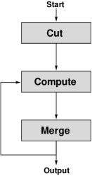
Figure 5: structure of the algorithm refined for SPM

This operation does not affect the theoretical complexity, as the number of intervals can be as high as the number of columns, but in practice the gain is very important (very few intervals are actually of size 1, and they tend to disappear upon iterations).

At each iteration of the merge step, the algorithm tries to combine intervals by considering the difference of height at their borders. If the merge succeeds, then new values are computed for the new interval.

When looking at the border between two intervals $I_{i}$ and $I_{i+1}$, there are two possibilities.

• Either $q_{i}\leq p_{i+1}+1$, in which case nothing can happen at the border. There are no cliffs inside the intervals by construction of the fixed point, hence nothing has to be done.

• Or $q_{i}\geq p_{i+1}+2$, which means that the system rule can be applied at the border. To obtain a new fixed point, the two intervals will be merged into $I^{\prime}_{\alpha(i)}=I_{i}\cup I_{i+1}$, where $\alpha$ is some suitable renumbering function. Remark that from one iteration to another, some intervals disappear (merge) and some remain, introducing lag in the indices.

  By Lemma 10, in this new interval the configuration belongs to $\mathcal{G}_{(n_{i}+n_{i+1})}^{l_{i}+l_{i+1}}$. Indeed, there is at most one plateau in $I_{i}$, at most another one in $I_{i+1}$, and they are separated by the cliff at the border. Therefore, the previous formulas still hold in the new interval $I_{\alpha(i)}$ with

  $$\begin{array}[]{rcl}n^{\prime}_{\alpha(i)}&=&n_{i}+n_{i+1}\\ l^{\prime}_{\alpha(i)}&=&l_{i}+l_{i+1}\\ c^{\prime}_{\alpha(i)}&=&(c_{i},c_{i+1})\enspace.\\ \end{array}$$

  Due to the fact that we are in the lattice $\mathcal{G}_{(n^{\prime}_{\alpha(i)})}^{l^{\prime}_{\alpha(i)}}$, we know that the computed fixed point will be correct. Therefore this operation can efficiently merge two intervals.

Once two intervals have merged, the interval list has to be updated with the new interval which replaces the two old ones. That way, the next iteration will act on the new list. This allows a newly created interval to merge at the next step, letting grains move as far as possible.

5.2 Transient length

For SPM, the algorithm can also compute the transient length. It is not possible in general because all paths from the root to the fixed point may not have the same length (IPM$(k)$ for example), but it is the case with SPM. So the number of steps simulated by the algorithm will correspond to the transient length, independently from the choice of the intervals.

To compute its value inside an interval, we associate to every sand grain a number corresponding to its movement, as in [2]. All these elementary values are added, supposing the configuration in Figure 3 has been reached. Then we have to subtract the “movement” weight $t^{0}$ of the initial configuration. One finds

$$t=\sum_{i=0}^{l-1}i(p-i)+\sum_{i=l-k}^{l-1}i-t^{0}=\frac{l(l-1)(3p-2l+1)}{6}+\frac{k(2l-k-1)}{2}-t^{0}\enspace,$$ (2)

where $t^{0}=\sum_{i=0}^{l-1}i\cdot a_{i+j}$ can be computed during the cut step; $j$ is the index of the leftmost column of the interval under consideration.

Remark 3

Again, the quantity $k$ is not really a number of grains. The rightmost sum of Equation (2) can be too big, but this will be compensated by a smaller value on the left. The extra grain added on the right is counted as a negative grain on the left.

One has to add all these values, over each interval at each iteration, to obtain the total transient length. When intervals do not merge, $t$ does not change. Otherwise, we are going to count the number of steps simulated, and subtract everything that had already been done during last iteration.

$$\begin{array}[]{@{}rcl@{}}t^{\prime}_{\alpha(i)}&=&\dfrac{1}{2}l^{\prime}_{\alpha(i)}\left(l^{\prime}_{\alpha(i)}-1\right)\left(3p^{\prime}_{\alpha(i)}-2l^{\prime}_{\alpha(i)}+1\right)+\dfrac{1}{2}k^{\prime}_{\alpha(i)}\left(2l^{\prime}_{\alpha(i)}-k^{\prime}_{\alpha(i)}-1\right)\\[4.30554pt] &-&t_{i}-t_{i+1}-n_{i+1}\cdot l_{i}\end{array}$$

The last term is the number of steps spent to move $n_{i+1}$ grains from interval $I_{i}$ to $I_{i+1}$.

5.3 Summary

Table 1 sums up all the calculations that have to be computed at each iteration, in the SPM example. The notation $\beta_{i}^{j}$ represents the value of the variable $\beta$ in the $i^{\textrm{\scriptsize th}}$ interval at the $j^{\textrm{\scriptsize th}}$ iteration.

$$\begin{array}[]{@{}c||c|c@{}}&\textrm{{A}}&\textrm{{B}}\\ \hline\cr\hline\cr I_{\alpha_{j}(i)}^{j+1}&I_{i}^{j}&I_{i}^{j}\cup I_{i+1}^{j}\\ \hline\cr n_{\alpha_{j}(i)}^{j+1}&n_{i}^{j}&n_{i}^{j}+n_{i+1}^{j}\\ \hline\cr l_{\alpha_{j}(i)}^{j+1}&l_{i}^{j}&\left\{\begin{array}[]{l@{\hspace{0.5cm}}l}\left\lceil\dfrac{1}{2}\left(\sqrt{8n_{\alpha_{j}(i)}^{j+1}+1}-1\right)\right\rceil\hfil\hskip 14.22636pt&\textrm{if $I_{i+1}^{j}$ is the last interval}\\[8.61108pt] l_{i}^{j}+l_{i+1}^{j}\hfil\hskip 14.22636pt&\textrm{otherwise}\end{array}\right.\\ \hline\cr p_{\alpha_{j}(i)}^{j+1}&p_{i}^{j}&\left\lfloor\dfrac{n_{\alpha_{j}(i)}^{j+1}}{l_{\alpha_{j}(i)}^{j+1}}+\dfrac{l_{\alpha_{j}(i)}^{j+1}}{2}-\dfrac{1}{2}\right\rfloor\\ \hline\cr q_{\alpha_{j}(i)}^{j+1}&q_{i}^{j}&\left\lceil\dfrac{n_{\alpha_{j}(i)}^{j+1}}{l_{\alpha_{j}(i)}^{j+1}}-\dfrac{l_{\alpha_{j}(i)}^{j+1}}{2}+\dfrac{1}{2}\right\rceil\\ \hline\cr k_{\alpha_{j}(i)}^{j+1}&k_{i}^{j}&n_{\alpha_{j}(i)}^{j+1}-\dfrac{1}{2}l_{\alpha_{j}(i)}^{j+1}\left(2p_{\alpha_{j}(i)}^{j+1}+1-l_{\alpha_{j}(i)}^{j+1}\right)\\ \hline\cr t_{\alpha_{j}(i)}^{j+1}&t_{i}^{j}&\begin{array}[]{l}\dfrac{1}{2}l^{j+1}_{\alpha_{j}(i)}\left(l^{j+1}_{\alpha_{j}(i)}-1\right)\left(3p^{j+1}_{\alpha_{j}(i)}-2l^{j+1}_{\alpha_{j}(i)}+1\right)\\[4.30554pt] \qquad{}+\dfrac{1}{2}k^{j+1}_{\alpha_{j}(i)}\left(2l^{j+1}_{\alpha_{j}(i)}-k^{j+1}_{\alpha_{j}(i)}-1\right)-t_{i}^{j}-t_{i+1}^{j}-n_{i+1}^{j}\cdot l_{i}^{j}\end{array}\end{array}$$

Table 1: summary of the operations performed by the algorithm modified for SPM, during one iteration. Column A contains the values obtained when $q_{i}^{j}\leq p_{i+1}^{j}+1$, and B the values for $q_{i}^{j}\geq p_{i+1}^{j}+2$.

At the end of the execution, these values allow to determine exactly the shape of the fixed point ($p$, $q$ and $k$ in each interval), and the total transient length.

5.4 Complexity (for SPM)

As seen above, the theoretical complexity is not improved with the modified algorithm, but we can refine the computation made in Section 4.4.

The compute and merge steps both consist in a scan of the intervals, hence they are in $\mathcal{O}(l)$. The number of iterations is clearly bounded by $\mathcal{O}(l)$, because there can not be more merging than the number of intervals. Moreover, the following proposition shows that it is also bounded by the number of grains. This last constraint becomes interesting when grains are scattered along the configuration, i.e. when $l\gg n$.

Proposition 16

Consider a configuration with $n$ grains. The algorithm finds the fixed point performing at most $\mathcal{O}(n)$ merge steps.

Proof.  It suffices to prove that if there are $m$ mergings, then there are at least $m$ grains in the configuration. Indeed, in order for $I_{i}$ and $I_{i+1}$ to merge we shall have $q_{i}\geq p_{i+1}+2\geq 2$. This means that $I_{i}$ has at least two grains in its rightmost column, mark the lowest one. After the merging, the marked grain does not move because it is at height $1$; moreover, it is not anymore at the border of two intervals. Therefore, any successive merging will mark a different grain, which has not been marked yet. Thus, there are no more than $n$ mergings. ❏

The following example shows that the bound given in Proposition 16 can be reached.

Example 1

Consider a configuration $c$ of length $l$ defined as follows

$$\forall i\in\left\{1,\ldots,l\right\},\;c_{i}=\left\{\begin{array}[]{l@{\hspace{1cm}}l}7\hfil\hskip 28.45274pt&\textrm{if $i=4j\ ,\quad 0\leq j<4\lfloor n/7\rfloor$}\\ n\mod 7\hfil\hskip 28.45274pt&\textrm{if $i=4\lfloor n/7\rfloor$}\\ 0\hfil\hskip 28.45274pt&\textrm{otherwise.}\end{array}\right.$$

In other words, $c=(7,0,0,0,7,0,0,0,\ldots,7,0,0,0,n\mod 7)$ (figure 6). The cut step produces $2\lceil n/7\rceil-1$ intervals of type $(7,0,0)$ and $(0)$. After the compute step, the configuration is $c^{\prime}=(3,2,2,0,3,2,2,0,\ldots,3,2,2,0,x_{1},x_{2},x_{3})$. One can easily see that there will be $\lceil n/7\rceil-1$ mergings of intervals of type $(3,2,2)$ and $(0)$ (in red, dashed dotted lines), in order to obtain the fixed point $(3,2,1,1,$ $3,2,1,1,\ldots,3,2,1,1,x_{1},x_{2},x_{3})$.

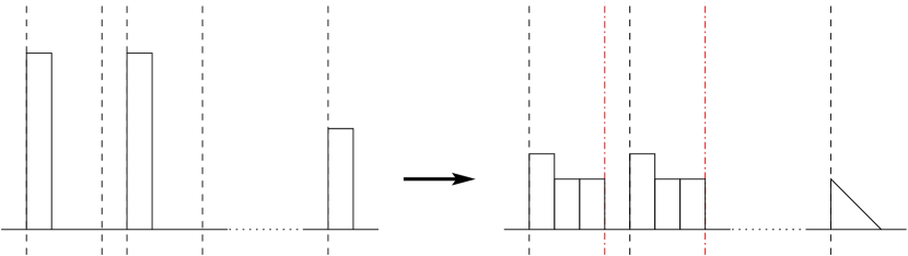
Figure 6: example of configuration reaching the $\mathcal{O}(n)$ complexity

Our algorithm computes the fixed point of any initial configuration in time $\mathcal{O}(l\cdot\min(n,l))$. There is a gain of at least $\sqrt{n}$ compared to the naive simulation, whose complexity is $\mathcal{O}(l\cdot n^{3/2})$ ($n^{3/2}$ is the number of avalanches, while $l$ corresponds to the scan of the configuration in order to find a cliff).

6 Conclusions

In this paper we proposed an algorithm for finding the fixed points of a large class of sandpile models starting from arbitrary finite configurations.

Time complexity of the algorithm depends on the structure of the initial configuration and, of course, on the model chosen. It might be interesting to build hierarchies of models classified according to time complexity of the (specialized version of the) algorithm, and study the algebraic property of the induced orbit graphs.

Another research direction consists in the study of models which allow grains to move in more than one direction and in parallel execution mode. Remark in fact that grains in a sandpile are essentially subject to two different type of forces: a vertical one due to gravity, and a horizontal one due to wind. Realistic models should consider both forces, and apply them in parallel to every grain. Our algorithm would be adapted to such models, and would allow much faster computation of this kind of natural phenomenon. Our research currently consists in finding such a model, with the needed lattice structure.

References

- [1] P. Bak, C. Tang, and K. Wiesenfeld. Self-organized criticality. Physical Review A, 38(1):364–374, 1988.
- [2] E. Goles and M. A. Kiwi. Games on line graphs and sand piles. Theoretical Computer Science, 115(2):321–349, 1993.
- [3] E. Goles and M. A. Kiwi. Sand-pile dynamics in a one-dimensional bounded lattice. In Cellular Automata and Cooperative Systems, volume 396 of NATO Science series C: Mathematical and Physical Sciences, pages 211–225. Kluwer Academic, 1993.
- [4] E. Goles, M. Latapy, C. Magnien, M. Morvan, and H. D. Phan. Sandpile models and lattices: a comprehensive survey. Theoretical Computer Science, 322:383–407, 2004.
- [5] E. Goles, M. Morvan, and H. D. Phan. Sand piles and order structure of integer partitions. Discrete Applied Mathematics, 117:51–64, 2002.
- [6] H. D. Phan. Structures ordonnées et dynamiques de piles de sable. PhD thesis, Université Paris VII, 1999.