A Statistical Framework for Efficient Monitoring of End-to-End Network Properties

Abstract.

Network service providers and customers are often concerned with aggregate performance measures that span multiple network paths. Unfortunately, forming such network-wide measures can be difficult, due to the issues of scale involved. In particular, the number of paths grows too rapidly with the number of endpoints to make exhaustive measurement practical. As a result, it is of interest to explore the feasibility of methods that dramatically reduce the number of paths measured in such situations while maintaining acceptable accuracy.

In previous work we have proposed a statistical framework for efficiently addressing this problem, in the context of additive metrics such as delay and loss rate, for which the per-path metric is a sum of per-link measures (possibly under appropriate transformation). The key to our method lies in the observation and exploitation of the fact that network paths show significant redundancy (sharing of common links).

In this paper we make three contributions: (1) we generalize the framework to make it more immediately applicable to network measurements encountered in practice; (2) we demonstrate that the observed path redundancy upon which our method is based is robust to variation in key network conditions and characteristics, including the presence of link failures; and (3) we show how the framework may be applied to address three practical problems of interest to network providers and customers, using data from an operating network. In particular, we show how appropriate selection of small sets of path measurements can be used to accurately estimate network-wide averages of path delays, to reliably detect network anomalies, and to effectively make a choice between alternative sub-networks, as a customer choosing between two providers or two ingress points into a provider network.

1. Introduction

In many situations it is important to obtain a network-wide view of path metrics such as latency and packet loss rate. For example, in overlay networks regular measurement of path properties is used to select alternate routes. At the IP level, path property measurements can be used to monitor network health, assess user experience, and choose between alternate providers, among other applications. Typical examples of systems performing such measurements include the NLANR AMP project, the RIPE Test-Traffic Project, and the Internet End-to-end Performance Monitoring project [11, 12, 8].

Unfortunately extending such efforts to large networks can be difficult, because the number of network paths grows as the square of the number of network endpoints. Initial work in this area has found that it is possible to reduce the number of end-to-end measurements to the number of “virtual links” (identifiable link subsets) — which typically grows more slowly than the the number of paths — and yet still recover the complete set of end-to-end path properties exactly [2, 13].

This result is based on a linear algebraic analysis of routing matrices, as pioneered in [13]. A routing matrix is a binary matrix that specifies which links appear in which end-to-end paths. Such a matrix $G$ has size (# paths) $\times$ (# links), and $G_{i,j}=1$ if and only if link $j$ is found along the route taken by path $i$. The rank of $G$, which is generally equal to the number of independent paths in the network, tends to be much smaller than the total number of paths. Since a maximal set of such independent paths can be used to reconstruct any other path in the network, it is sufficient to monitor only this set. Algorithms for choosing such a set have been developed [13, 2], based on linear algebraic methods of subset selection.

In previous work we have proposed a general approach to extending this strategy. First, we note that routing matrices encountered in practice generally show significant sharing of links between paths. One implication is that routing matrices have small effective rank compared to their actual rank — a small set of eigenvalues of $G^{T}G$ tend to be much larger than the rest. Next, we propose a statistical framework for approximating summary path metrics which can be used to exploit the property of low effective rank of routing matrices.

The statistical framework we have developed draws on linear model theory. Linear model theory is concerned with the statistical inference of quantities that are related through some underlying linear relationship. In this case, we are concerned with the inference of path properties, which are related through their linear dependence on link properties. Linear model theory provides a well developed set of tools that allow one in many cases to construct and analyze procedures for making optimal linear inferences.

While our previous work has developed a framework for attacking the problem, there are a number of hurdles, both theoretical and practical, separating our simple model from application to realistic network settings. Our goal in this paper is to eliminate those hurdles. We do so by a combination of analysis, experimentation, and application to real network data. In the process, we demonstrate the power of the resulting framework for solving problems of real interest to network operators and users.

Our first contribution concerns the generality of our methods. Our initial, simple analysis relied on a model in which link metrics are assumed to have equal variance. This property does not hold in practice; in reality, the variance of link delay (for example) can vary considerably from link to link, depending on phenomena such as localized congestion. It is important to understand how the structure of our proposed solution changes when link metrics have unequal variance, as occurs in practice. We first present the analysis of this more general case and show how to incorporate this more realistic property into our framework.

As previously mentioned, the opportunity for efficient network-wide measurement derives from the small effective rank of routing matrices. However the factors that determine this phenomenon are not fully understood. Thus it is important to ask whether the low effective rank of routing matrices is a robust property. This property can be affected in at least two ways: first, if links fail, the degree of link sharing among paths is affected; and second, if link metrics have unequal variance, the benefits of link sharing may be reduced. Our second contribution is an evaluation of how effective rank changes when network links fail, and when links have unequal variance. We show that, even in the presence of significant differences in variance across links, unequal link variance does not generally diminish the utility of our methods.

Since our goal is to move our methods into practical use, and to demonstrate their utility, it is appropriate to apply them to data obtained from a real network. For that purpose we employ a large set of measurements from the NLANR Active Measurement Project (AMP). These are comprised of per-hop delay measurements; we select the subset of these measurements traversing the Abilene network. Throughout the paper we assess our analytic assumptions as well as the actual performance of our methods using this data.

Our work is motivated by a number of current problems in network measurement. Many projects are currently using all-pairs path measurement, including [11, 12, 9]. To the extent that such projects intend to either measure network-wide health or detect anomalous network conditions, we hope that our methods can enable more efficient measurement strategies. With respect to measurements of subnetworks, research such as [1] has shown that significant performance benefits can accrue when a customer chooses the best path from among a set of alternatives made available by multihoming.

To demonstrate our applicability to these sorts of problems, we evaluate the performance of our methods on Abilene data for a number of specific cases. The first problem is that of obtaining network-wide averages of per-path delay, as would be needed for a network “health” measure. We show that a very accurate estimate of average path delay (with relative error typically less than 1%) is obtained using as few as one-tenth of the paths needed for exact measurement. In addition, we show that our extended methods that incorporate unequal link variance are more accurate than the simpler methods in our previous work.

Our second problem concerns the detection of anomalies within the network. We are interested in detecting when average network performance exceeds a threshold, such as three standard deviations from its mean. We show that reasonable anomaly detection can be done with a very small subset of networks paths — as few as only one-third of the paths needed for exact measurement.

Our final problem concerns the problem of selecting between two network ingress points. In this setting, a network customer or peer has multiple connection points to the network of interest and needs to choose between them for accessing a given set of destinations. We show that, once again, only a small set of paths need to be measured in order to accurately choose between the alternatives.

The rest of the paper is organized as follows. In Section 2 we review previous work in this area and provide necessary background. Then in Section 3 we present our analytic results, which extend our previous methods to the case of unequal link variance. Next in Section 4 we describe the data used in evaluating our methods. In Section 5 we evaluate the robustness of low effective rank of routing matrices, and in Section 6 we describe the results of applying our methods to the three real-world problems. Finally in 7 we conclude.

2. Background

In this section we formally define the path estimation problem and discuss previous work that has addressed it. Let $\mathcal{G}=(\mathcal{V},\mathcal{E})$ be a strongly connected directed graph, where the nodes in $\mathcal{V}$ represent network devices and the edges in $\mathcal{E}$ represent links between those devices. Additionally, let $\mathcal{P}$ be the set of all paths in the network. Let $n_{v}=\lvert\mathcal{V}\rvert$, $n_{e}=\lvert\mathcal{E}\rvert$, $n_{p}=\lvert\mathcal{P}\rvert$ denote respectively the number of devices, links and paths.

We will consider a metric measured on the paths $i\in\mathcal{P}$ whose value $y\in\mathbf{R}^{n_{p}}$ is a linear function of the value $x\in\mathbf{R}^{n_{e}}$ of the same metric on the edges $j\in\mathcal{E}$. In particular, we are interested in the case where $n_{p}\gg n_{e}$ and the linear relation between $y$ and $x$ is given by $y=Gx$, where $G\in\{0,1\}^{n_{p}\times n_{e}}$ is a routing matrix whose entries simply indicate the traversal of a given link by a given path, so that

(1) $$G_{i,j}=\begin{cases}1&\text{if path $i$ traverses link $j$}\\ 0&\text{otherwise.}\end{cases}$$

For example, if we let $x$ denote the delay times for edges in the network and let $y$ denote the delay times for paths in the network, then $y=Gx$. A similar relation holds, under suitable transformation, between path-wise and link-wise loss rates.

As explained in Section 1, our interest in this paper focuses on the problem of monitoring global network properties via measurements on some small subset of the paths. Earlier work by Chen and colleagues [2] shows that in fact one need measure only a number of paths $k^{*}$ on the order of the number of links in the network, to still be able to recover exact knowledge of all network path behaviors. Their argument is essentially linear algebraic in nature, and is based upon the fact that a subset, say $\tilde{G}$, of only $k^{*}=\operatorname{Rank}(G)$ independent rows of $G$ are sufficient to span the image of $G$ i.e., $\{y\in\mathbf{R}^{n_{p}}:y=Gx,x\in\mathbf{R}^{n_{e}}\}$. As a result, given the measurements for paths corresponding to the rows in such a $\tilde{G}$, measurements for all other paths may be obtained as a function thereof. Similar work may be found in [10], in the context of Boolean algebras, for the problem of detecting link failures.

Following on their work in [2], Chen and colleagues showed [3] that the number $k^{*}$ of paths needed for their method scales at worst like $O(n_{v}\log n_{v})$ in a collection of real and simulated networks. Furthermore, they argue that this behavior is to be expected in internet networks, due to the high degree of sharing of paths as they traverse common routes in the dense core.

In our previous work [5], such sharing was noted as well. However, there it was shown that the effective rank of $G$ can in fact be arguably much less than the actual rank. As a result, we proposed that substantially greater savings can be achieved by allowing for the approximate monitoring of path metrics and adopting an approach based on predictive linear statistical methods.

As an illustration, consider the Abilene network, a high-performance network which serves Internet2 (the U.S. national research and education backbone). A map of this network is shown in Figure 1(a). The network can be seen to consist of $11$ nodes, at locations across the continental United States, but only $2\times 15=30$ directed links. Accordingly, a large amount of sharing of these links can be expected of the $11\times 10=110$ paths on the network.

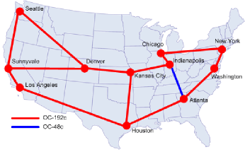
(a) Map of Abilene

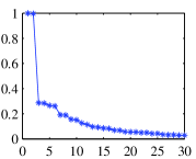
(b) Eigenspectrum of $G$

Figure 1. Map of the Abilene network and the eigenspectrum of one of its routing matrices.

Our work goes beyond these observations to point out that in fact, some links are shared much more highly than others. The effect can be evaluated via the eigenspectrum of the routing matrix. In Figure 1(b) is shown the eigenspectrum of a routing matrix $G$ for this network. More specifically, we have plotted the (ordered) eigenvalues of the symmetric, non-negative definite matrix $G^{T}G$. Since all $30$ of these eigenvalues are positive, we have that $\operatorname{Rank}(G)=30$, and therefore, recalling the results in [2, 3], no more than $30$ paths need to be measured in order to recover exact knowledge of an additive metric $y$. However, the decay in the spectrum in Figure 1(b) — particularly the sharp decay in the early portion — suggests that the effective rank of $G$ may be a good deal less than 30, perhaps on the order of 10 or so. Algebraically, this means that the span of the rows of $G$ exists primarily (but not entirely) in a subspace of $\mathbf{R}^{n_{p}}$ of dimension potentially much lower than 30. From a practical perspective, this means that accurate (but not exact) recovery of $y$ may be possible based on measurements from much fewer than 30 paths.

We have confirmed this behavior of the routing matrix $G$ in additional real networks of varying and substantial sizes; and we have exploited the decay in these matrices in developing a framework for efficient monitoring of paths based on statistical prediction, in which measurements from measured paths are used to predict those on unmeasured paths [5]. However, this earlier work was developed in the context of a relatively simple model, in which link measurements were assumed to be uncorrelated and to share a single, common variance. Additionally, the resulting methodology was only validated through analytics and numerical simulations. Nevertheless, these validations suggested a strong potential for the underlying concept; here we show that that potential is realizable.

3. Efficient Monitoring

In this section we describe a linear statistical framework for prediction of end-to-end properties. This is a general framework, which includes our previous work as a special case and is more immediately applicable to real-life data. Additionally, it uses a correspondingly different criterion for selecting which paths to measure, one that incorporates information on both path sharing and relative variability of the metric on links. The impact of these changes is not only analytic or abstract; there can be a substantial effect on the selection of paths, as we illustrate in Section 5.1.

3.1. Statistical Prediction

We begin by building a model for the end-to-end properties in $y$. In the work that follows, it is necessary only that the first two moments of $x$ and $y$ be specified, as opposed to a full distributional specification. Let $\mu$ be the mean of $x$ and let $\Sigma$ to be the covariance of $x$. Then the corresponding statistics for $y$ are simply $\nu=G\mu$ and $V=G\Sigma G^{T}$, respectively.

Now fix $k\leq\operatorname{Rank}(G)$. Let $y_{s}\in\mathbf{R}^{k}$ denote the values $y_{i_{1}},\dots,y_{i_{k}}$ of the metric of interest for $k$ paths $i_{1},\dots,i_{k}\in\mathcal{P}$ that are to be sampled (i.e., measured), and let $y_{r}\in\mathbf{R}^{n_{p}-k}$ denote the values for those $n_{p}-k$ paths that remain. Similarly, let $G_{s}$ be those rows of $G$ corresponding to the $k$ paths, $i_{1},\dots,i_{k}$ and let $G_{r}$ be the remaining rows. Then we may partition $y$ and $G$ into

(2) $$y=\begin{bmatrix}y_{s}\\ y_{r}\end{bmatrix}\text{\quad{}and\quad}G=\begin{bmatrix}G_{s}\\ G_{r}\end{bmatrix}\text{,}$$

and we may similarly re-express the mean and covariance of $y$ as

(3) $$\nu=\begin{bmatrix}\nu_{s}\\ \nu_{r}\end{bmatrix}=\begin{bmatrix}G_{s}\mu\\ G_{r}\mu\end{bmatrix}$$

and

(4) $$V=\begin{bmatrix}V_{ss}&V_{sr}\\ V_{rs}&V_{rr}\end{bmatrix}=\begin{bmatrix}G_{s}\Sigma G_{s}^{T}&G_{s}\Sigma G_{r}^{T}\\ G_{r}\Sigma G_{s}^{T}&G_{r}\Sigma G_{r}^{T}\end{bmatrix}\text{.}$$

In this paper, we take as our monitoring goal the task of obtaining accurate (approximate) knowledge of a linear summary of network path conditions. That is, we seek to accurately predict a linear function of the path conditions $y$, of the form $l^{T}y$ where $l\in\mathbf{R}^{n_{p}}$, based on the measurements in $y_{s}$. Two such linear summaries are the network-wide average, given by $l^{T}y$ for $l_{i}\equiv 1/n_{p}$, and the difference between two groups of paths $\mathcal{P}_{1}$ and $\mathcal{P}_{2}$, given by

(5) $$l_{i}=\begin{cases}1/\lvert\mathcal{P}_{1}\rvert&\text{if $i\in\mathcal{P}_{1}$}\\ -1/\lvert\mathcal{P}_{2}\rvert&\text{if $i\in\mathcal{P}_{2}$}\\ 0&\text{otherwise.}\end{cases}$$

The prediction of $l^{T}y$, from the $k$ sampled path values in $y_{s}$, can be viewed as a particular instance of the classical problem of prediction in the statistical literature on sampling [14].

If the mean-squared prediction error (MSPE) is used to judge the quality of a predictor i.e., if the quality of a predictor $p(y_{s})$ is measured by $E[(l^{T}y-p(y_{s}))^{2}]$, then the best predictor is known to be given by the conditional expectation

(6) $$E[l^{T}y|y_{s}]=l_{s}^{T}y_{s}+E[l_{r}^{T}y_{r}|y_{s}],$$

where $l_{s}$ and $l_{r}$ are defined similarly to $y_{s}$ and $y_{r}$, respectively. But this requires knowledge of the joint distributional structure. It is therefore common practice to restrict attention to a smaller and simpler subclass of predictors, with the class of linear predictors being a natural choice. In this case, the best linear predictor (BLP) is given by the expression

(7) $$a^{T}y_{s}=l_{s}^{T}y_{s}+l_{r}^{T}G_{r}\mu+l_{r}^{T}c_{*}(y_{s}-G_{s}\mu)\text{,}$$

where $c_{*}$ is any solution to $c_{*}V_{ss}=V_{rs}$. (The derivation of this result follows similarly to the analogous result for simple linear statistical models given in [4, VI.3].)

However, without knowledge of $\mu$, the BLP in (7) is an ideal that cannot be computed. One natural solution is to estimate $\mu$ from the data. This is a version of the network tomography problem, and in some sense the reverse of the well-known traffic-matrix estimation problem. There are many versions of this problem, and many methods for solving them. See [6], for example. We will use a simple method based on generalized least squares to estimate the mean $\mu$ as

(8) $$\hat{\mu}=[G_{s}^{T}V_{ss}^{-1}G_{s}]^{-}G_{s}^{T}V_{ss}^{-1}y_{s}\text{.}$$

Here $M^{-}$ denotes a generalized inverse of the matrix $M$.

Substituting $\hat{\mu}$ for $\mu$ in (7) produces an estimate of the BLP (an E-BLP) that is a function of only the measurements $y_{s}$, the routing matrix $G$ and the link covariance matrix $\Sigma$. Specifically, we obtain

(9) $$\begin{split}\hat{a}^{T}y_{s}&=l_{s}^{T}y_{s}+l_{r}^{T}G_{r}[G_{s}^{T}V_{ss}^{-1}G_{s}]^{-}G_{s}^{T}V_{ss}^{-1}y_{s}\\ &=l_{s}^{T}y_{s}+l_{r}^{T}V_{rs}V_{ss}^{-1}y_{s}\text{.}\end{split}$$

The first expression in (9) can be reduced to the second using properties of generalized inverses and projection matrices. The derivation of these and the other expressions above requires only that $V_{ss}$ be invertible and that $\Sigma$ be positive definite.

As a side point, it is useful to note that the form of our E-BLP also follows from application of the arguments in [5] to the transformed problem $y=(GC)(C^{-1}x)\equiv\tilde{G}\tilde{x}$, where $C$ is a non-singular matrix deriving from the factorization $\Sigma=CC^{T}$. The effect of this transformation is to introduce the variable $\tilde{x}$, with mean $C^{-1}\mu$ and covariance $I$, whose simplified covariance structure then follows that assumed for the calculations in [5].

3.2. Path Selection

The material in Section 3.1 assumes a set of measurements from $k$ paths $i_{1},\ldots,i_{k}\in\mathcal{P}$. However, given the resources to measure any $k$ paths in a network, we are still faced with the question of which $k$ paths to measure. A natural response would be to choose $k$ paths that minimize $\operatorname{MSPE}(\hat{a}^{T}y_{s})$, over all subsets of $k$ paths. This quantity can be shown to have the form

(10) $$\begin{split}\operatorname{MSPE}(\hat{a}^{T}y_{s})&=\operatorname{MSPE}(a^{T}y_{s})+(\operatorname{Bias}\hat{a}^{T}y_{s})^{2}\end{split}$$

where

(11) $$\operatorname{MSPE}(a^{T}y_{s})=l_{r}^{T}\left(V_{rr}-V_{rs}V_{ss}^{-1}V_{sr}\right)l_{r}$$

and

(12) $$\operatorname{Bias}(\hat{a}^{T}y_{s})=l_{r}^{T}\left(V_{rs}V_{ss}^{-1}G_{s}-G_{r}\right)\mu\text{.}$$

We see that the error inherent in our E-BLP, $\hat{a}^{T}y_{s}$, is equal to that of the BLP, $a^{T}y_{s}$, which is an unbiased predictor, plus the bias that accompanies the need to estimate $\mu$. Accordingly, the expression for $\operatorname{Bias}(\hat{a}^{T}y_{s})$ involves both the mean $\mu$ and the covariance $\Sigma$ for the unseen link measurements $x$, whereas that for $\operatorname{MSPE}(a^{T}y_{s})$ involves only the covariance.

Of course, since we typically do not have knowledge of $\mu$, minimization of the full expression for $\operatorname{MSPE}(\hat{a}^{T}y_{s})$ in (10) is an unrealistic goal in practice. Instead, if adequate information on the covariance matrix $\Sigma$ is available, one might consider trying to minimize the expression for $\operatorname{MSPE}(a^{T}y_{s})$ in (11). A useful equivalent expression for this MSPE is

(13) $$\operatorname{MSPE}(a^{T}y_{s})=l_{r}^{T}(G_{r}C)(I-B_{s})(G_{r}C)^{T}l_{r}\text{,}$$

where

(14) $$\begin{split}B_{s}&=(G_{s}C)^{T}[(G_{s}C)(G_{s}C)^{T}]^{-1}(G_{s}C)\\ &=C^{T}G_{s}^{T}V_{ss}^{-1}G_{s}C\end{split}$$

is the orthogonal projection onto $\operatorname{Row}(G_{s}C)$. Since orthogonal projection matrices are idempotent and symmetric, the MSPE in (13) can be seen to be the square of the Euclidean norm of the projection of $(G_{r}C)^{T}l_{r}$ onto $\operatorname{Row}(G_{s}C)^{\perp}=\operatorname{Null}(G_{s}C)$.

The nature of the space $\operatorname{Row}(G_{s}C)$ obviously will depend on $G$, $C$, and the manner in which they interact through multiplication of the latter by the former. Here, motivated by our examination of the covariance structure of the edge delay data in Section 4, we consider in detail the case where $\Sigma$ is a diagonal matrix. We leave the problem of path selection for non-diagonal covariance as an interesting open problem.

To begin, suppose that $\Sigma=I$ and consider the case of predicting the metric on a single path that lies outside of the sample ($l_{s}$ all zeros and $l_{r}$ containing a single one). In this case we have $C=I$, so the MSPE simply measures the degree to which the row of $G$ corresponding to the single path lies outside of $\operatorname{Row}(G_{s})$. Of course, if our goal is only to monitor the value $y_{i}$ for a single path $i\in\mathcal{P}$, then the most efficient strategy would be simply to measure $y_{i}$. However, we are interested here in strategies that allow for the capacity to do whole-network monitoring, in which case the minimization of (13), when $C=I$ and $l$ is nontrivial, can be interpreted roughly as seeking a subset of $k$ paths for whom the rows in $G_{s}$ capture as many of the rows of $G$ as possible to the largest extent possible. This situation corresponds to that studied in [5].

Now take the case where $\Sigma$ is an arbitrary diagonal matrix. The matrix $C$ is then also diagonal and the columns of $GC$, which correspond to links in the network, are the columns of $G$ rescaled by the variability of the corresponding link. That is, each non-zero entry in a given row of $G$, indicating that the corresponding path passes over a given link, is replaced by the standard deviation of the metric on that link. Therefore, we see that minimization of the MSPE in the case of diagonal $\Sigma$ is analogous to the case of $\Sigma=I$, but with the important difference that the routing information for each path is augmented with information on the variability among the links over which it travels, thus allowing for the relative weight among these links to differ. We will see in Section 5.1 that the incorporation of such variance information can have a nontrivial effect on which paths are selected.

From the standpoint of optimization theory, our path-selection problem may be viewed as an example of the so-called ‘subset selection’ problem in computational linear algebra. In the two cases just described, the selection of an appropriate subset of rows of $GC$ has a meaningful physical interpretation, in terms of the selection of paths, and vice versa. Exact solutions to this problem are computationally infeasible (it is known to be NP-complete), but the problem is well-studied and an assortment of methods for calculating approximate solutions have been offered.

The method we have used for the empirical work in this paper was adapted from the subset selection method described in Algorithm 12.1.1 of [7], and is a modified version of that described in our previous work [5]. Specifically, we first compute a singular value decomposition $GC=U\Delta V^{T}$ for $GC$. The columns of the matrix $U$ form an orthogonal basis for the span of $GC$, with the relative importance of each column indicated by the magnitude of the corresponding singular value in the diagonal matrix $\Delta$. These values in turn are simply the square-root of the eigenvalues of $(GC)^{T}(GC)$, through which the connection with the discussion on reduced-rank in Section 2 is evident. Ideally, we seek a subset of $k$ paths for which the corresponding rows of $GC$ span the first $k$ singular dimensions. We make heuristic use of a QR-factorization with column pivoting to pursue this task, writing $U_{(k)}^{T}P_{k}=QR$, where $U_{(k)}$ is an $n_{p}\times k$ matrix formed from the first $k$ columns of $U$ and $P_{k}$ is an $n_{p}\times n_{p}$ permutation matrix defined by the column pivoting. We then take $G_{s}$ to be the submatrix of $G$ formed by the first $k$ rows of $P_{k}^{T}G$.

It should be noted that $P_{k}$ has to be recomputed for different values of $k$. However, the overall complexity for the computation of E-BLP in (9) is dominated by the computation of the SVD of $GC$ which is $O(n_{p}^{2}n_{e})$. This can likely be improved through the use of methods for sparse matrices, since the entries of $GC$ tend to include a large fraction of zeros. The other components are the QR-factorization with column pivoting which is $O(k^{2}n_{p})$ and the computation of $V_{ss}^{-1}$ which is only $O(k^{3})$.

4. Data: Abilene Path Delays

Our methods are applicable to any per-link metric that adds to form per-path metrics. To demonstrate a concrete example we take per-link delays for Abilene.

4.1. Collection and Processing

Our data comes from the NLANR Active Measurement Project. This project continually performs traceroutes between all pairs of AMP monitors on ten minute intervals. Because most AMP monitors are on networks with Abilene connections, most traceroutes pass over Abilene. This provides a highly detailed view of the state of the Abilene network. Our data consists of the set of all measurements taken over 3 days in 2003, yielding 432 time points.

For each time period, we start with traceroutes between the 14917 pairs of monitors for which complete data was available. From this set we construct estimates of a consistent set of delays for each link within the Abilene network. Links comprising the Abilene network were identified by their known interface addresses. Since different traceroutes traverse each link at slightly different times, and since each traceroute takes up to three measurements per hop, we form a single estimate of each link’s delay by averaging across all the traceroutes that measured that link in the current time point. This yields a single measure of delay for each link and timepoint; while this measure does not capture the variations in delay that occur within a ten minute interval, it provides a realistic and representative value for delay that can be used to construct path-wise metrics.

Note that in practice, our methods do not make use of per-link measurements; we only need to form them for validation purposes. Thus, issues with accurate measurement of per-link delays do not represent a limitation of our methods.

4.2. Data Characteristics

In our data, the mean delays for Abilene’s $30$ directed edges are evenly spread out from 2 to 36 milliseconds, with standard deviations that run from 0.16 to 0.94 for the full three-day period. Other than a diurnal cycle in some of the edges, we found nothing remarkable in the structure of the edge delays. There is no apparent relationship between the edge delays and the standard deviations; edges with similar means exhibit both large and small standard deviations.

In order to learn more about the relationships between the edge delays themselves, we looked at the covariance matrix for one day’s worth of data. The entries in this matrix are primarily dominated by the diagonal elements, with a small number of off-diagonal entries of similar magnitude. However, inspection of the actual delay data on the links involved in the large off-diagonals leads us to believe that these cases are actually artifacts of the measurement procedure.

Note that our framework in Section 3 requires knowledge of the covariance matrix, which in practice could be obtained from either historical data or possibly periodic, infrequent measurement of the edges. For the purposes of this paper, and motivated by the findings mentioned just above, we will take $\Sigma$ to be a diagonal covariance matrix with non-zero entries given by the variances of the edge delay data over one day.

5. Robustness of Path Redundancy

Critical to the success of our proposed methodology is the degree to which some subset of independent rows in $GC$, denoted $G_{s}C$ above, can effectively approximate the span of the full set of rows in $GC$. Since multiplication by a diagonal $C$ does not change the linear relations between the rows of $G$, this boils down to an issue of path redundancy. In order for path redundancy to translate into reduced measurement frameworks with dependable implementation and performance characteristics, it needs to be a robust property. We examine that robustness here by looking at the effect of two factors: (1) inclusion of information on link variances, via the matrix $C$, and (2) network integrity. We find the redundancy in the cases we study to be quite robust.

5.1. Effect of Link Covariance

The path selection scheme proposed in this paper takes into account not only the sharing among paths, but also the relative variances of the link measurements. Therefore, it is natural to ask to what degree inclusion of the information on the link measurement variances affects the relative rank involved. Analysis of the Abilene data provides evidence to suggest that the phenomenon of reduced rank should remain robust to the incorporation of link variance information that varies across a moderate range, while that information in turn can lead to meaningful adjustments in the finer details of the path selection process.

Our analysis is based primarily on a comparison of the behavior of the eigenvalues and eigenvectors of the matrix $(GC)^{T}(GC)$, in the two cases of $\Sigma=I$ and $\Sigma$ the diagonal matrix described in Section 4.2. The eigenspectra of $GC$ for these two cases, shown in Figure 2, are quite similar. In particular, they exhibit similar decay, which suggests a corresponding similarity in the relative ranks of $G$ and $GC$. In turn, we may therefore expect similar relative performance for a given number of measured paths. This expectation is found to be fulfilled in the application presented in Section 6.1.

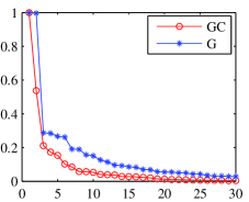
Figure 2. Comparison of eigenspectra for $G$ and $GC$ on Abilene.

However, despite their similarity, the two spectra are not identical, and it is interesting to explore further the reasons for and the implications of their differences. For example, note that in the spectra for $G^{T}G$ there appears to be a pattern of pairing among the larger eigenvalues, whereas this pattern is absent from the spectra of $(GC)^{T}(GC)$ in the case of $\Sigma$ diagonal. The pairing in the case of the former derives from the fact that the routing is symmetric under the particular routing matrix $G$ we obtained. The lack of pairing in the case of the latter is a reflection of the unequal link variances. This observation is supported by an examination of the first two eigenvectors in our two models, shown in Figure 3, in conjunction with the Abilene map, which reveals that in both cases their energy is concentrated on links making up both directions of the northern transcontinental route—particularly in the region of Indianapolis. But an examination of the variances in our diagonal model shows that the edges along the eastbound route, in particular Kansas City–Indianapolis (edge 16), generally have larger variances than their westbound counterparts. Hence the gap between the first and second eigenvalues in this model, and the concentration of the energy of the first eigenvector of $(GC)^{T}(GC)$ on the edges of the eastbound route.

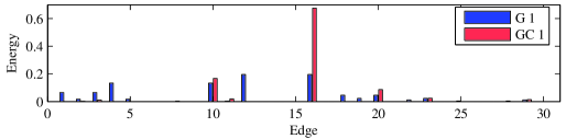
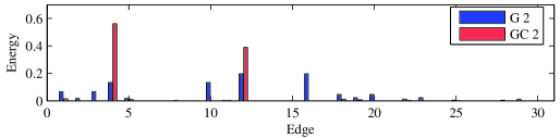
Figure 3. Comparison of the energy distribution of first two eigenvectors of $G^{T}G$ and $(GC)^{T}(GC)$. Top Figure: First eigenvector of $G^{T}G$ versus the first eigenvector vector of $(GC)^{T}(GC)$. Bottom Figure: Second eigenvector of $G^{T}G$ versus the second eigenvector of $(GC)^{T}(GC)$. (See Appendix A for a list of edges.)

Further insight into the effect of link variance information can be obtained by looking at the actual paths selected by our algorithm under each choice of $\Sigma$. These are shown in Figure 4. Each column corresponds to a path, and the markers in a given row $k$ indicate which $k$ paths are selected. The paths have been grouped according to their starting node; the ten paths within each group are sorted by destination using the same ordering. So for example, the first column in the Chicago group corresponds to the Chicago–Seattle path.

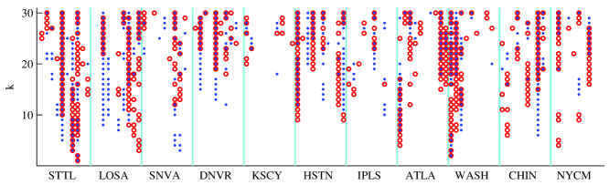
Figure 4. Subset selection for $\Sigma=I$ compared to selection for diagonal $\Sigma$. The markers in each row represent the paths chosen for the size $k$ sample when $\Sigma=I$ (red circles) and when $\Sigma$ is diagonal (blue dots).

A number of interesting characteristics may be observed. A large fraction of the chosen paths are found to match, particularly for larger $k$. However, under the diagonal $\Sigma$ there does seem to be a slightly increased emphasis on eastward paths, as might be expected from our earlier discussion. When the paths do differ, often the change in paths will be minor, in the sense that the ingress point remains the same and the egress point changes to a neighboring node (red circles next to blue dots). Similarly, other times the ingress point will move to a geographical “neighbor”. This behavior is especially apparent in the case of smaller values of $k$; for example in $k=3$ to $6$ the eastward paths from Los Angeles are traded for eastward paths starting in Sunnyvale.

5.2. Effect of Link Failures

The analysis just described is for the Abilene routing matrix when the network is fully intact. Failures of links within a network are to be expected, however, and our method should be robust to such failures. In particular, it is to be hoped that the reduced rank of $GC$ persists sufficiently under the failure of a link(s) to allow for the continued use of a (possibly altered) reduced subset of paths for monitoring. An analysis of our Abilene data suggests that a substantial degree of robustness can be expected for path redundancy in the face of normal link failures. That is, both the number of paths needed to capture a given portion of the span of $GC$ and the actual choice of paths appeared quite stable.

Proceeding as in Section 5.1, we pursued these issues by examining the behavior of the eigenvalues and eigenvectors of $GC$. First consider the case of a single link failure. Starting with a set of IGP weights for Abilene, we deleted one link and used Dijkstra’s algorithm to compute the shortest paths between cities. These paths were then used to construct a routing matrix $G$ for the modified network. The spectrum of $GC$ for each of the 30 resulting routing matrices, scaled to all have maximum eigenvalue $1$, are plotted in Figure 5. Impressively, the spectra appear to be quite stable. A similar plot is shown in Figure 5 for the case of two link deletions. While the stability of the spectra is less than in the previous case, it is still substantial when one considers that Abilene is a small network with only $30$ links. Note that, in the absence of real data for each of the modified networks, we have used a diagonal $\Sigma$ for the intact Abilene network throughout this section.

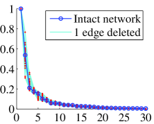
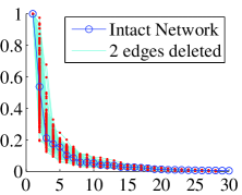
Figure 5. Spectra for $GC$ of Abilene delay data, after the deletion of (a) one or (b) two links. In Figure (b) the spectra for the 18 graphs that are not strongly connected are not displayed. Each spectrum has been rescaled so that the first eigenvalue is one.

The stability we have observed in the spectra of Figure 5 indicates that even if a link or two goes down in the Abilene network, the number of paths one needs to measure for a given level of accuracy remains essentially unchanged. But this conclusion still leaves unanswered the question of which paths should be used. To address this question, we examine the stability of the energy distribution of the first eigenvector of $(GC)^{T}(GC)$. Specifically, in Figure 6 we present the corresponding energy distributions following the deletion of one link, for each of the 30 links, as described above. The boxplots indicate that, generally, the energy distribution is quite stable under link deletions; each box is centered tightly along the energy distribution of the first eigenvector for the intact network.

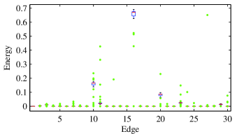
Figure 6. Boxplots of the energy distribution in the first eigenvector of $(GC)^{T}(GC)$ after one link deletion. The red bars represent the median and the green dots represent outliers. Note that many boxes have no height and are hidden behind the outliers.

There are, however, a certain number of outliers, indicating that certain particular edge deletions can have a notable effect. For example, one such outlier occurs when we delete edge 16 (Kansas City–Indianapolis), which is the highest-energy link for the intact network. In this instance, the bulk of the energy is moved to the link between Los Angeles and Houston, followed by a smaller allotment to that between Houston and Atlanta. This change would seem to indicate a shift from the northern transcontinental route to the southern one. Conversely, deletion of the link between Indianapolis and Chicago (edge 10) causes a good portion of the energy to shift to the link between Indianapolis and Atlanta. These observations suggest that a shift to the southern route occurs only when absolutely necessary.

6. Applications

In this section, we show how our framework may be applied to address three practical problems of interest to network providers and customers. In particular, we show how the appropriate selection of small sets of path measurements can be used to accurately estimate network-wide averages of path delays, to reliably detect network anomalies, and to effectively make a choice between alternative sub-networks, as a customer choosing between two providers or two ingress points into a provider network.

6.1. Monitoring a Network-wide Average

An average is perhaps the most basic network-wide quantity that one might be interested in monitoring. So as our first application, we consider the prediction of the average delay over all paths.

Recall from Section 4 that our data consist of delays on all $n_{p}=110$ paths of the Abilene network, for each of 432 ten-minute epochs over three consecutive days. Using (9), with $l_{i}\equiv 1/n_{p}$, we computed predictions of the network-wide average path delay during each epoch, for a choice of $k=1,\ldots,30$ measured paths, where the paths were chosen using the algorithm described in Section 3.2. Both the case of $\Sigma=I$ and the case of a general diagonal $\Sigma$ were examined, where the values for the latter derive from the analysis described in Section 4.2. To summarize the accuracy of our predictions, we calculated the average relative error for each $k$, where the average is taken over epochs. The results are shown in Figure 7.

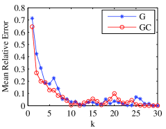
Figure 7. Mean relative prediction error as a function of $k$.

Two conclusions are particularly apparent. First, we see that for both variance models increasing the number $k$ of paths measured improves the accuracy of the prediction up until around $k=9$ or $10$, after which it basically levels out. Since it is roughly at this point that the spectra of the (weighted) routing matrices level out as well, this suggests that our subset selection algorithm is indeed doing what we are asking of it, in that it is tracking the effective rank quite closely. Second, we note that the method based on general diagonal $\Sigma$ typically outperforms that based on the more restricted assumption of $\Sigma=I$, again up until around $k=9$ or $10$, after which the relative performances oscillate in a fairly random manner. This indicates explicitly the gain that can be gotten by incorporating more accurate variance information into the model where, for example, the relative error in the more general model is on the order of just $5\%$ by $k=9$.

To get a better idea of how well the various predictors are doing, we can compare plots of the predictions against a plot of the actual mean delays, as shown in Figure 8 for $k=3,5,7,$ and $9$. Note that all of the predictions mirror the rise and fall of the actual network-wide delay quite closely — even for as few as $k=3$ measured paths, for which the correlation between the two time-series is $\rho=0.814$. However, it also is clear that there is a downward bias in these predictions, and that this bias is increasingly prominent as $k$ decreases. Therefore, some manner of bias correction is needed.

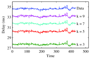
Figure 8. Predictions of network-wide average path delays, for various choices of $k$.

The source of this bias can be traced to a lack of information on links in the network that end up being traversed by none of the $k$ measured paths. In fact, the generalized inverse used in our E-BLP in (9) simply estimates the corresponding values $x_{j}$ on these links to be zero. Hence, as the measured paths reach a point where every link contributes to at least one path, as it does by roughly $k=10$, the bias diminishes accordingly. Note, however, that the bias for each $k$ in Figure 8 is fairly constant. This suggests that a small amount of additional measurement information could go a long way.

We implemented a simple method of bias correction, in which we assume access to full link measurements $x$ for the first of our 432 epochs. This corresponds to a one-time use of path measurements among a sufficient set of paths for complete reconstruction of link delays (in this case, 30 paths). Since it is a one-time-only measurement, it represents a minimal addition to the network measurement load. The bias of our predictions in the first epoch was then calculated, through comparison of the predictions with the actual path values $y$, which follow from the reconstructed link values via $y=Gx$. This correction was then used to adjust all other predictions in the other 431 epochs, which amounts to simply shifting each curve in Figure 8 upward a certain amount. Boxplots of the relative bias remaining after application of this procedure are shown in Figure 9. The predictions are now extremely accurate, being off usually by less than $0.3\%$, and almost always within $1\%$ — even when as few as only $k=3$ paths are measured.

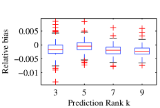
Figure 9. Relative bias after bias correction.

6.2. Anomaly Detection

The application in Section 6.1 evaluates the predictor by standard statistical summaries, in essence looking at the accuracy of the predictor at hitting an unknown target. But it is also important to evaluate the accuracy in terms of accomplishing higher-level tasks. One such higher-level task of importance is the detection of potentially anomalous events.

For the purposes of this application, we will define an anomaly as a spike in the delay time that deviates from the average of the previous six measurements (corresponding to one hour) by more than a specified threshold. For example, the red dots in Figure 11 indicate points at which the mean path delay exceeds the mean of the previous six epochs by more than three standard deviations.

To predict when such anomalies occur, we look for spikes in the predicted values. These predictions are highly correlated with the actual mean path delays. For example, the $k=9$ prediction exhibits a correlation coefficient of $\rho=0.930$. Recall that while a strong correlation implies a strongly linear relation between the prediction and the actual values, this does not mean the dynamic range of the two signals are identical. Thus we find it useful to explore the effects of both $k$ and the detection threshold applied to the predicted values.

Insight on the choice of $k$ and threshold for the predictor can be obtained by examining ROC (Receiver Operating Characteristic) curves such as those in Figure 10. These plots of the true positive rate against the false positive rate for different parameter values are a common tool for establishing cutoff values for detection tests. Each curve in Figure 10 is formed by taking one value for $k$ and varying the threshold level. Examining these curves, one sees that for a given threshold, say $1\sigma$, the true positive rate increases with the sample size $k$ while the false positive rate stays about the same. Working with a $k=9$ prediction, we see that the upper-left corner of the ROC curve (the best trade-off between a low false positive rate and a high true positive rate) occurs at around $2\sigma$.

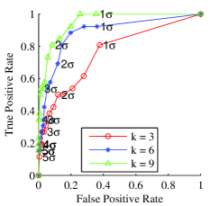
Figure 10. ROC curves for predicting $3\sigma$ spikes. The threshold used to predict the spikes is varied from $1\sigma$ to $5\sigma$ in increments of $0.25\sigma$.

In Figure 11, the results are shown for the case $k=9$, with a threshold of $2\sigma$. Circles have been placed along the actual path delay time series at the epochs that were flagged as anomalies in the predicted time series. On the whole, this predictor is quite accurate. Most of the major spikes are flagged, resulting in a true positive rate of 81%, while the false positive rate is only 8%. Furthermore, most of these false positives seem to occur at lesser spikes in the actual delay data.

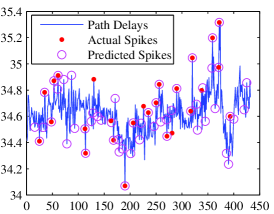
Figure 11. Comparison of predicted and actual spikes. The real spikes are those that exceed 3 times the standard deviation of the previous 6 epochs. The predicted spikes are those epochs where the rank 9 prediction exceeds 2 times the standard deviation of its previous 6 epochs.

6.3. Subnetwork Comparison

The applications in Sections 6.1 and 6.2 both involved predictions of an average over the entire Abilene network. However, it is important to note that there is nothing in our framework that requires that it be applied to a full network. It applies equally to arbitrary subnetworks and, as we will show now, can be particularly useful for the task of subnetwork comparison.

Specifically, consider the problem of comparing the average delay times for the paths in two groups, each consisting of all paths that originate at a given node. This is an increasingly common scenario in the Internet. For example, many customers now seek to optimize their access to the Internet via multihoming, and choosing the best network ingress connection dynamically based on changing network conditions. Another case occurs when providers peer at multiple locations and thus have more than one ingress to a peer network.

Let $\mathcal{P}_{1}$ and $\mathcal{P}_{2}$ denote the two sets of paths that we wish to compare. If these measurements are being taken by a customer choosing between two providers, then the only paths available for sampling are probably those paths that belong to either $\mathcal{P}_{1}$ or $\mathcal{P}_{2}$. To ensure that we choose only from among those paths, we restrict the routing matrix to a matrix $\tilde{G}$ which contains only the rows of $G$ that correspond to paths in $\mathcal{P}_{1}$ and $\mathcal{P}_{2}$.

To determine which collection of paths has a shorter mean delay, we define $l$ via

(15) $$l_{i}=\begin{cases}1/\lvert\mathcal{P}_{1}\rvert&\text{ if path $i$ is in }\mathcal{P}_{1}\\ -1/\lvert\mathcal{P}_{2}\rvert&\text{ if path $i$ is in }\mathcal{P}_{2}\text{,}\end{cases}$$

so that $l^{T}y$ is the difference between the mean delay of the paths in $\mathcal{P}_{1}$ and the mean delay of the paths in $\mathcal{P}_{2}$. The sign of $l^{T}y$ is therefore of interest. When $l^{T}y$ is negative, $\mathcal{P}_{1}$ has a lower average delay, and when $l^{T}y$ is positive, $\mathcal{P}_{2}$ has the lower average delay. To predict the sign of $l^{T}y$ we can use (9) to compute $\hat{a}^{T}y_{s}$ and check its sign.

To illustrate, we chose Chicago and Atlanta as our two ingress points. The spectrum of $\tilde{G}C$, shown in Figure 12, has a strong decay with a knee somewhere around $k=5$. So our path selection method was applied to $\tilde{G}C$ with $k=5$, and we used the measurements on these five paths to predict the difference in mean path delays out of Chicago and Atlanta.

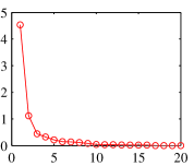
Figure 12. Spectrum of $\tilde{G}C$ for the subnetwork comparison between Chicago and Atlanta.

In Figure 13, we compare the predicted delay difference against the actual delay difference. The predictor tracks the actual delay difference very well, with a correlation coefficient of $\rho=0.866$, and the ingress point with a shorter mean delay is predicted (via the sign of $\hat{a}^{T}y_{s}$) correctly 79.6% of the time.

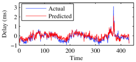
Figure 13. Subnetwork comparison between paths starting at Chicago and those starting at Atlanta. Prediction from a sample of 5 paths, with a correction for bias.

A good part of this roughly $11\%$ rate of error is due to the noise in the time-series. A multihomed user is not likely to switch between providers on a minute-to-minute basis, but rather might base decisions on predictions in a window of some length of time into the past. To approximate this behavior, we apply an exponential smoothing (with $\alpha=0.1$) to both the predicted and actual differences in average delays. As can be seen in Figure 14, the prediction tracks the actual delay difference very well, and the ingress point with a shorter mean delay is now correctly predicted over 88% of the time.

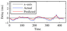
Figure 14. Exponential smoothing ($\alpha=0.1$) of the predicted and actual time series in Figure 13.

We looked at the times at which the smoothed predictor and actual delay differ in sign, and found that such periods fall into two categories. First, there are minor periods where one series will dip below or above zero for no more than an hour. Alternatively, the predictor will be slightly early or late in changing sign. The offset is usually less than an hour, other than one notable exception between $t=267$ and $t=283$ where the actual difference hovers just below zero.

Lastly, we point out that this performance in some sense carries even more weight when one considers the fact that this predictor for the Chicago/Atlanta pairing has a correlation with the actual difference that is in the bottom quartile, over all pairs of ingress points, as can be seen by examining Figure 15.

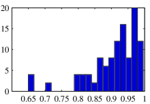
Figure 15. Correlations between unsmoothed predicted and actual differences in the mean delay for subnetworks. All predictions use $k=5$.

7. Conclusion

In this paper we have demonstrated, using real data from an operating network, that it is possible to monitor end-to-end network delay properties quite accurately using a subset of paths substantially smaller than that needed for exact monitoring. We have illustrated the relevance of our approach through the development of three practical applications of interest to network providers and customers: monitoring the ‘health’ of a network, anomaly detection, and comparison of subnetworks.

The framework proposed in this paper casts the problem of efficient network monitoring as one of statistical prediction. Our approach exploits an observed redundancy in links traversed by paths in real networks. We explored the characteristics of this redundancy and found them to be robust to variations in the state of the network, such as link failure.

Our next steps include evaluation of our methods in a larger live network such as PlanetLab. Additionally, it would be of interest to better understand the factors underlying the observed path redundancy in the networks we have examined, and the manner in which they contribute to the decay of the eigenspectra of the corresponding routing matrices. Initial insight into such issues is beginning to emerge in works such as [3].

8. Acknowledgements

The authors would like to thank Anukool Lakhina (Computer Science Department, Boston University) for his help with collecting and processing the data.

Appendix A Abilene Edges

Table 1 lists the edges of Abilene in the order that they appear in Figures 3 and 6.

#	Edge
1	New York–Chicago
2	New York–Washington D.C.
3	Chicago–New York
4	Chicago–Indianapolis
5	Washington D.C.–New York
6	Washington D.C.–Atlanta
7	Atlanta–Washington D.C.
8	Atlanta–Indianapolis
9	Atlanta–Houston
10	Indianapolis–Chicago
11	Indianapolis–Atlanta
12	Indianapolis–Kansas City
13	Houston–Atlanta
14	Houston–Kansas City
15	Houston–Los Angeles
16	Kansas City–Indianapolis
17	Kansas City–Houston
18	Kansas City–Denver
19	Kansas City–Sunnyvale
20	Denver–Kansas City
21	Denver–Sunnyvale
22	Denver–Seattle
23	Sunnyvale–Kansas City
24	Sunnyvale–Denver
25	Sunnyvale–Los Angeles
26	Sunnyvale–Seattle
27	Los Angeles–Houston
28	Los Angeles–Sunnyvale
29	Seattle–Denver
30	Seattle–Sunnyvale

Table 1. Abilene’s directed edges.

References

- [1] A. Akella, S. Seshan, and A. Shaikh. Multihoming performance benefits: An experimental evaluation of practical enterprise startegies. In USENIX, 2004.
- [2] Y. Chen, D. Bindel, and R. H. Katz. Tomography-based overlay network monitoring. In Proceedings of the 2003 ACM SIGCOMM conference on Internet measurement, pages 216–231. ACM Press, 2003.
- [3] Y. Chen, D. Bindel, H. Song, and R. H. Katz. An algebraic approach to practical and scaleable overlay network monitoring. In Proceedings of the 2004 ACM SIGCOMM. ACM Press, 2004.
- [4] R. Christensen. Plane answers to complex questions. Springer-Verlag, New York, 1987.
- [5] D. B. Chua, E. D. Kolaczyk, and M. Crovella. Efficient estimation of end-to-end network properties. In Proceedings of IEEE INFOCOM 2005, (to appear).
- [6] M. Coates, A. Hero, R. Nowak, and B. Yu. Internet tomography. IEEE Signal Processing Magazine, May 2002.
- [7] G. H. Golub and C. F. V. Loan. Matrix Computations. Johns Hopkins University Press, Baltimore, Maryland, 1983.
- [8] Internet End-to-end Performance Monitoring Project. http://www-iepm.slac.stanford.edu/.
- [9] Internet Traffic Report. http://www.internettrafficreport.com.
- [10] H. X. Nguyen and P. Thiran. Active measurement for multiple link failures: Diagnosis in IP networks. In Proceedings of the Passive and Active Measurements Workshop. Springer Verlag, 2004.
- [11] NLANR Active Measurement Project. http://amp.nlanr.net/AMP/.
- [12] RIPE Test-Traffic Project. http://www.ripe.net/test-traffic/.
- [13] Y. Shavitt, X. Sun, A. Wool, and B. Yener. Computing the unmeasured: An algebraic approach to internet mapping. In IEEE INFOCOM 2001, April 2001.
- [14] R. Valian, A. H. Dorfman, and R. M. Royall. Finite Population Sampling and Inference: A prediction approach. Wiley Interscience, 2000.