Minimum Dilation Stars

Abstract

The dilation of a Euclidean graph is defined as the ratio of distance in the graph divided by distance in $\mathbb{R}^{d}$. In this paper we consider the problem of positioning the root of a star such that the dilation of the resulting star is minimal. We present a deterministic $O(n\log n)$-time algorithm for evaluating the dilation of a given star; a randomized $O(n\log n)$ expected-time algorithm for finding an optimal center in $\mathbb{R}^{d}$; and for the case $d=2$, a randomized $O(n\,2^{\alpha(n)}\log^{2}n)$ expected-time algorithm for finding an optimal center among the input points.

1 Introduction

A star is a graph with exactly one internal vertex, called its center; it has edges from the center to every external vertex, and no other edges. The dilation between any pair of vertices $a$ and $b$ in a Euclidean graph is defined [5] as the cost of the shortest path from $a$ to $b$, divided by the Euclidean distance $|ab|$. The dilation of a graph is defined as the maximum dilation over all pairs of vertices. We consider the following problem: for any fixed $d\geq 2$, given a set $V\subset\mathbb{R}^{d}$ of $n$ points, construct a star with center $c\in\mathbb{R}^{d}$ and leaves $V$ such that the star has minimal dilation. We present algorithms for the case when $c$ is constrained to be one of the input points, as well as the unconstrained case when $c$ may be any point in $\mathbb{R}^{d}$.

We present algorithms to evaluate the dilation of a given star in $O(n\log n)$ time; find the optimal center $c\in\mathbb{R}^{d}$ for a given set of external vertices in $O(n\log n)$ expected time; and for a set of vertices $V\subset\mathbb{R}^{2}$, select an optimal center $c\in V$ in expected $O(n\,2^{\alpha(n)}\log^{2}n)$ time. The evaluation algorithm’s task is to find the single pair of points that define the graph’s dilation. It works by identifying $O(n)$ pairs of points with the potential to be that pair in $O(n\log n)$ time, and evaluating the dilation for each of those $O(n)$ point pairs. Our algorithm for the unconstrained optimization algorithm formulates the problem as a quasiconvex program, and uses the evaluation algorithm as a component of Timothy Chan’s randomized optimization framework [3] to arrive at the solution in $O(n\log n)$ expected time. The algorithm for the constrained case works by repeatedly selecting a random vertex, evaluating the dilation that would result from using that vertex as the center, computing the region $R$ of space that could contain a center yielding an even lower dilation, and discarding all the vertices outside $R$. This procedure is iterated an expected $O(\log n)$ times, and computing a description of $R$ takes $O(n\,2^{\alpha(n)}\log n)$ time, resulting in an $O(n\,2^{\alpha(n)}\log^{2}n)$ expected-time algorithm.

Finding a minimum dilation star can be viewed as an instance of the classic facility location problem [4]: given a set of demand sites and supply sites, find a center minimizing a particular objective function. In our case the objective function is defined as the maximum dilation between any pair of points. This formulation could e.g. represent the problem of deciding where to position an airline hub, such that flights with layovers are not unreasonably longer than direct flights.

Narasimhan and Smid [8] considered the related problem of computing dilation approximately. They present algorithms which can compute an $\varepsilon$-approximation of the dilation of a path in $O(n\log n)$ time, a cycle in $O(n\log n)$ time, and a tree in $O(n\log^{2}n)$ time, for any fixed $d\geq 1$. Agarwal et al. [1] considered the problem of computing the dilation of a polygonal curve. They present algorithms to compute the exact dilation of a polygonal curve in $\mathbb{R}^{2}$ in $O(n\log n)$ expected time, or in $\mathbb{R}^{3}$ in subquadratic time. Langerman et al. [7] presented algorithms which compute the dilation of a planar polygonal curve in expected $O(n\log n)$ time, a planar tree in $O(n\log^{2}n)$ time, or a planar cycle in $O(n^{\frac{3}{2}}\log n)$ time. The evaluation algorithm presented in this paper computes the exact dilation of a star in $O(n\log n)$ time for any fixed $d\geq 2$.

2 The evaluation problem

Formally, the evaluation problem is as follows: given a set $V$ of $n$ points in $\mathbb{R}^{d}$ and a point $c\in\mathbb{R}^{d}$, compute the dilation of the Euclidean star with center $c$ and leaves $V$.

For any pair of vertices $a$ and $b$, a star contains exactly one path from $a$ to $b$: the path $\langle a,c,b\rangle$. So the dilation between $a$ and $b$ is

$$\Delta_{c}(a,b)=\frac{|ac|+|cb|}{|ab|}$$

where $|ac|$ designates the Euclidean distance from $a$ to $c$.

The dilation of the star is

$$\Delta_{c}=\max_{a,b\in V}{\Delta_{c}(a,b)}\enspace.$$

Define $\hat{a}$ to be one of the points in $V$ for which $\Delta_{c}(a,\hat{a})$ is greatest (there may be more than one pair of points with dilation $\Delta_{c}$). As noted in the introduction, one approach to solving this problem is to reason that for any $a\in V$, $\hat{a}$ could be any of the $n-1$ points in $V\setminus\{a\}$. Then $\Delta_{c}$ may be computed by an algorithm that evaluates $\Delta_{c}(a,b)$ for all $O(n^{2})$ pairs of points. As we will see, this approach is overly conservative. In this section we present an algorithm that identifies $O(n)$ candidate pairs of points, such that the pair $(a,\hat{a})$ for which $\Delta_{c}=\Delta_{c}(a,\hat{a})$ is guaranteed to be one of the candidates. The algorithm takes $O(n\log n)$ time to generate the candidate list, and computing the largest dilation among $O(n)$ pairs of points takes $O(n)$ time. The point pairs are identified using two techniques, each generating $O(n)$ pairs. One technique generates a list of $O(n)$ pairs of points guaranteed to contain $(a,\hat{a})$ when $\Delta_{c}$ is high; the other generates $O(n)$ pairs guaranteed to contain $(a,\hat{a})$ when $\Delta_{c}$ is low.

2.1 The high dilation case

One of our heuristics for finding $\hat{a}$ is to identify $a$’s $k$ nearest neighbors, for a constant $k\in O(1)$. This heuristic is guaranteed to identify $\hat{a}$ when $\Delta_{c}=\Delta_{c}(a,\hat{a})$ is high; formally, we will prove that if $\Delta_{c}\geq\Gamma$ for a constant $\Gamma>3$, then $\hat{a}$ is one of $a$’s $k$ nearest neighbors, for a constant $k$. The $k$ nearest neighbors of every $a\in V$ may be reported in $O(kn\log n)$ time using the algorithm of Vaidya [10], so the process of identifying these $O(n)$ point pairs takes $O(n\log n)$ time.

Lemma 1

Suppose $a\in V$ and $\Delta_{c}=\Delta_{c}(a,\hat{a})\geq\Gamma$ for a constant $\Gamma>3$. Then $|ac|\geq\phi|a\hat{a}|$ for a constant $\phi>1$ that depends only on $\Gamma$.

Proof 2.1.

By definition,

$$\Gamma\leq\Delta_{c}=\frac{|ac|+|c\hat{a}|}{|a\hat{a}|}\leq\frac{|ac|+(|ac|+|a\hat{a}|)}{|a\hat{a}|}\leq 1+2\frac{|ac|}{|a\hat{a}|}\enspace,$$

so

$$|ac|\geq\frac{\Gamma-1}{2}|a\hat{a}|\enspace.$$

Therefore if $\Gamma>3$, $\phi=\frac{\Gamma-1}{2}>1$.

Lemma 2.2.

Suppose that $\Delta_{c}=\Delta_{c}(a,\hat{a})\geq\Gamma$ for a constant $\Gamma>3$, let $\kappa$ be the $d$-sphere centered on $a$ with radius $|a\hat{a}|$, and $u,v\in V$ be two input points inside $\kappa$. Then there is a constant $\gamma>0$ that depends only on $\Gamma$, such that $|uv|\geq\gamma|a\hat{a}|$.

Proof 2.3.

By Lemma 1, $|ac|-|a\hat{a}|\geq(1-1/\phi)|ac|$, so

$$\frac{3|ac|}{|a\hat{a}|} \geq \frac{|ac|+|\hat{a}c|}{|a\hat{a}|}=\Delta_{c}\geq\Delta_{c}(u,v)$$

$$\geq \frac{|uc|+|cv|}{|uv|}\geq\frac{2(|ac|-|a\hat{a}|)}{|uv|}$$

$$\geq \frac{2(1-1/\phi)|ac|}{|uv|}\enspace.$$

It follows that $|uv|\geq\frac{2}{3}(1-1/\phi)|a\hat{a}|$. So $|uv|\geq\gamma|a\hat{a}|$ for $\gamma=\frac{2}{3}(1-1/\phi)$; $\phi>1$ so $\gamma>0$.

Lemma 2.4.

If $\Delta_{c}\geq\Gamma$ and $\Delta_{c}=\Delta_{c}(a,\hat{a})$, then $\hat{a}$ is one of $a$’s $k$ nearest neighbors, for a constant $k$ depending only on $\Gamma$ and the dimension.

Proof 2.5.

As shown in Lemma 2.2, the distance between any $u$ and $v$ is proportional to the radius $r_{\kappa}=|a\hat{a}|$ of $\kappa$. Let $\sigma=\gamma/\sqrt{d}$ and partition $\kappa$ into small $d$-cubes with sides of length $\sigma r_{\kappa}$ (see Figure 1). Under such an arrangement no cube contains more than one input point. $\kappa$ can contain no more than $\lceil(\frac{2r_{\kappa}}{\sigma r_{\kappa}})^{d}\rceil=\lceil(\frac{2}{\sigma})^{d}\rceil$ such cubes, which is constant in $n$. So we may conclude that if $\Delta_{c}=\Delta_{c}(a,\hat{a})$ then $\hat{a}$ is one of $a$’s $k$ nearest neighbors, for a constant $k=\lceil(\frac{2}{\sigma})^{d}\rceil$.

Figure 1: $\kappa$ partitioned into small $d$-cubes for $d=2$.

2.2 The low dilation case

Our other heuristic for finding $\hat{a}$ is to identify points whose distance from $c$ is similar to that of $a$. This may be done by sorting $V$ by distance from $c$, then for each $a$, identifying the points whose indices in the sorted sequence are within $l$ of $a$’s, for a constant $l$. We will show that this heuristic is guaranteed to identify $\hat{a}$ when $\Delta_{c}=\Delta_{c}(a,\hat{a})$ is low, i.e., that if $\Delta_{c}\leq\Gamma$ for a constant $\Gamma$, and $V_{S}$ is the set $V$ sorted by distance from $c$, then for any $v_{i}\in V_{S}$, if $v_{j}=\hat{v_{i}}$ and $\Delta_{c}=\Delta_{c}(v_{i},v_{j})$ then $|i-j|\leq l$, for a constant $l$. We prove this by showing that space may be partitioned into $d$-dimensional annuli with exponentially growing radii, all centered on $c$, such that each annulus contains $O(1)$ points from $V$, and for any $a\in V$, $\hat{a}$ lies within one of $O(1)$ adjacent annuli. We define an annulus $A_{c,i}$ in terms of its inner and outer radii, $\rho^{i}$ and $\rho^{i+1}$, respectively,

$$A_{c,i}=\{p\in\mathbb{R}^{d}\enspace|\enspace\rho^{i}\leq|pc|\leq\rho^{i+1}\}$$

where the constant $\rho$ is defined as

$$\rho>\sqrt{\frac{\Delta_{c}+1}{\Delta_{c}-1}}\enspace.$$

Lemma 2.6.

If $a\in A_{c,i}$ and $\hat{a}\in A_{c,i+k}$, then $k\leq 2$.

Proof 2.7.

Suppose for the sake of contradiction that $k\geq 3$. We now establish an upper bound on $\Delta_{c}(a,\hat{a})$ by positioning $a$ and $\hat{a}$ such that dilation is maximized. This happens when $a$ and $\hat{a}$ are colinear and as close as possible. We may assume without loss of generality $|ac|\leq|\hat{a}c|$; so $|ac|=\rho^{i+1}$ and $|\hat{a}c|=\rho^{i+3}$, hence

$$\Delta_{c}(a,\hat{a}) = \frac{\rho^{i+1}+\rho^{i+3}}{\rho^{i+3}-\rho^{i+1}}$$

$$= \frac{1+\rho^{2}}{\rho^{2}-1}$$

$$< \frac{1+\frac{\Delta_{c}+1}{\Delta_{c}-1}}{\frac{\Delta_{c}+1}{\Delta_{c}-1}-1}=\frac{(\Delta_{c}-1)+\Delta_{c}+1}{\Delta_{c}+1-(\Delta_{c}-1)}=\Delta_{c}$$

which is a contradiction; so the assumption $k\geq 3$ must be false.

Lemma 2.8.

There exists a function $\theta_{MIN}$ such that if $a$ and $b$ lie in the same annulus, $\angle acb\geq\theta_{MIN}(\Delta_{c})$, and a value $\Delta_{0}$ such that for all $\Delta_{c}<\Delta_{0}$, $\theta_{MIN}(\Delta_{c})>\pi/2$.

Proof 2.9.

We wish to establish a lower bound on $\angle acb$, and so we consider the choice of $a$ and $b$ that makes $\angle acb$ as acute as possible. For a fixed $\Delta_{c}(a,b)$, we can do this by making $||ac|-|cb||$ as large as possible. Without loss of generality, assume $|cb|=\rho|ac|$; then

$$\Delta_{c}\geq\frac{|ac|+\rho|ac|}{|ab|}\enspace.$$

Let $\theta=\angle acb$; then by the law of cosines,

$$\Delta_{c} \geq \frac{|ac|+\rho|ac|}{\sqrt{|ac|^{2}+\rho^{2}|ac|^{2}-2\rho|ac|^{2}\cos\theta}}$$

$$\geq \frac{1+\rho}{\sqrt{1+\rho^{2}-2\rho\cos\theta}}\enspace.$$

Solving for $\theta$,

$$\theta\geq\cos^{-1}(\frac{\rho}{2}+\frac{1}{2\rho}-\frac{(1+\rho)^{2}}{2\rho\Delta_{c}^{2}})\enspace,$$

so we let $\theta_{MIN}(\Delta_{c})=\cos^{-1}(\frac{\rho}{2}+\frac{1}{2\rho}-\frac{(1+\rho)^{2}}{2\rho\Delta_{c}^{2}})$. The result follows from the convergence of the limit

$$\lim_{\Delta_{c}\rightarrow 1^{+}}\theta_{MIN}(\Delta_{c})=\pi\enspace.$$

Lemma 2.10.

Each $A_{c,i}$ contains $O(1)$ points from $V$.

Proof 2.11.

Lemma 2.8 shows that if $a$ and $b$ are in the same annulus and $\theta=\angle acb$, then

$$\theta\geq\theta_{0}=\min_{\Delta_{0}\leq\Delta_{c}\leq\Gamma}\theta_{MIN}(\Delta_{c})\enspace.$$

Thus each annulus contains $O(\theta_{0}^{1-d})$ points; $\theta_{0}$ and $d$ are constant with respect to $n$, so this quantity is as well.

Lemma 2.12.

If $\Delta_{c}\leq\Gamma$, $V_{S}$ is the set $V$ sorted by distance from $c$, $v_{s}$ and $v_{t}\in V_{S}$, and $\Delta_{c}=\Delta_{c}(v_{s},v_{t})$, then $|s-t|\leq l$ for a constant $l$ depending only on $\Gamma$ and $d$.

Proof 2.13.

Lemma 2.6 shows that if $a\in A_{c,i}$ and $\hat{a}\in A_{c,j}$, then $|i-j|\leq 2$. The points in contiguous annuli will be contiguous in $V_{S}$. So $\hat{a}$ must be within $l$ ranks of $a$ in $V_{S}$, where $l$ is the number of points that may lie in two annuli. As shown in Lemma 2.10, $l$ is constant with respect to $n$.

2.3 The evaluation algorithm

Theorem 2.14.

Given a set $V\subset\mathbb{R}^{d}$ of $n$ points and center $c\in\mathbb{R}^{d}$, it is possible to compute the dilation $\Delta_{c}$ for the star with center $c$ and leaves $V$ in $O(n\log n)$ time, provided $d$ is constant.

Proof 2.15.

We generate a list of $O(n)$ pairs of points as follows. Compute the $k$ nearest neighbors for the set $V$ in $O(n\log n)$ time, for the constant $k$ described in Subsection 2.1. Then for each $a\in V$, append the point pairs consisting of $a$ paired with each of $a$’s $k$ nearest neighbors to the list. Next, create $V_{S}$ by sorting the points in $V$ by distance from $c$ in $O(n\log n)$ time. For each $v_{i}\in V_{S}$, add the pair $(v_{i},v_{j})$ to the list, for every $j$ such that $|i-j|\leq l$, for the constant $l$ described in Subsection 2.2. The resulting list has $(kn+ln)\in O(n)$ elements. As shown in Lemmas 2.4 and 2.12, the pair defining the dilation of the star, $(a,\hat{a})$ such that $\Delta_{c}=\Delta_{c}(a,\hat{a})$, is certain to be present in the list. So we can compute $\Delta_{c}$ by evaluating the dilation of each of the $O(n)$ pairs of points, and returning the maximum.

3 The unconstrained
optimization problem

We now turn to the following problem: given a set of $n$ points $V\subset\mathbb{R}^{d}$, find a point $c$, not necessarily belonging to $V$, such that the star with center $c$ and leaves $V$ has minimal dilation.

3.1 Reduction to a quasiconvex program on $O(n^{2})$ contraints

A function $f:\mathbb{R}^{d}\mapsto\mathbb{R}$ is quasiconvex when its level sets $f^{\leq\lambda}=\{x\in\mathbb{R}^{d}\enspace|\enspace f(x)\leq\lambda\}$ are convex. Quasiconvex programming [6] is a generalization of linear programming: a quasiconvex program is a finite set $S$ of quasiconvex functions (constraints); the solution to a quasiconvex program is the input $x\in\mathbb{R}^{d}$ minimizing the objective function $f_{S}=\max_{f_{i}\in S}f_{i}(x)$. Amenta et al. showed [2] that if a solution to a constant-sized subset of $S$ may be solved in $O(1)$ time, then the program may be solved in $O(|S|)$ expected time.

Lemma 3.16.

The star center $c$ minimizing $\Delta_{c}$ may be computed by solving a quasiconvex program with $O(n^{2})$ constraints.

Proof 3.17.

We introduce one contraint $f_{i,j}:\mathbb{R}^{d}\mapsto\mathbb{R}$ for each pair of points $v_{i},v_{j}\in V$:

$$f_{i,j}(x)=\frac{|v_{i}x|+|xv_{j}|}{|v_{i}v_{j}|}\enspace.$$

Hence the solution $x$ is precisely the point $c$ for which the dilation is minimized for all pairs of input points.

The denominator of $f_{i,j}$ is the distance between $v_{i}$ and $v_{j}$, which is constant with respect to $x$. So $f_{i,j}(x)$ is proportional to the sum of the distances of $x$ from $v_{i}$ and $v_{j}$, or equivalently each $f_{i,j}$ defines an ellipsoid with foci $v_{i}$ and $v_{j}$. So any level set $f_{i,j}^{\leq\lambda}$ is elliptical (see Figure 2), and hence convex; so each $f_{i,j}$ is quasiconvex.

Figure 2: An example level set $f_{i,j}^{\leq\lambda}$.

3.2 The optimization algorithm

In this section we show how to solve the unconstrained optimization problem in $O(n\log n)$ expected time. We adapt Timothy Chan’s randomized optimization technique [3] to our problem. Chan states his result in terms of LP-type problems, but following [6], we rephrase it in terms of quasiconvex programming:

Lemma 3.18 (Chan).

Let $\cal Q$ be a space of quasiconvex functions, $\cal P$ be a space of input values, and $f:2^{\cal P}\mapsto 2^{\cal Q}$ map sets of input values to sets of functions in $\cal Q$. Further, suppose that $\cal P$, $f$, and $\cal S$ satisfy the following properties:

• There exists a constant-time subroutine for solving quasiconvex programs of the form $f(B)$ for any $B\subset\cal P$ with $|B|\in O(1)$.

• There exists a decision algorithm that takes as input a set $P\subset\cal P$ and a pair $(\lambda,\bar{x})$, and returns yes if and only if $q(\bar{x})\leq\lambda$ for all $q\in f(P)$. The running time of the decision algorithm is bounded by $D(|P|)$, where there exists a constant $\epsilon>0$ such that $D(n)/n^{\epsilon}$ is monotone increasing.

• There are constants $s$ and $r$ such that, for any input set $P\subset\cal P$, we can find in time at most $D(|P|)$ a collection of sets $P_{i}$, $0\leq i<r$, each of size at most $s|P|$, for which $f(P)=\cup_{i}f(P_{i})$.

Then for any $P\subset\cal P$ we can solve the quasiconvex program $f(P)$, where $|P|=n$, in randomized expected time $O(D(n))$.

We now show how to apply this result to the problem at hand.

Theorem 3.19.

Given a set $V$ of $n$ points, it is possible to compute a point $c$ that admits the minimal-dilation star with center $c$ and leaves $V$ in expected $O(n\log n)$ time.

Proof 3.20.

Lemma 3.16 shows how to formulate this problem as a LP-type program with quasiconvex constraints. Section 2 provides an $O(n\log n)$ time algorithm to evaluate the dilation of a star with $n$ leaves; so our decision algorithm can invoke that algorithm, then compare the result to $\lambda$, to decide whether $q(\bar{x})\leq\lambda$ for any $\lambda$. The resulting decision algorithm has running time $D(n)\in O(n\log n)$.

A set of input points $P$ may be divided into r subsets, each with size $\lceil s|P|\rceil$, as follows. To ensure correctness, every pairing of points must be mutually present in at least one $P_{i}$. So we partition $P$ into three arbitrary disjoint subsets $Q_{1},Q_{2},$ and $Q_{3}$, each of size $|Q_{i}|\geq\lfloor|P|/3\rfloor$, and form three subsets $P_{1}=P\setminus Q_{1}$, $P_{2}=P\setminus Q_{2}$, and $P_{3}=P\setminus Q_{3}$. Then any pair of points present in $P$ is also mutually present in some $P_{i}$. Each $P_{i}$ has size $|P_{i}|\leq\frac{2}{3}|P|$, so our approach fits the requirements of Chan’s framework with parameters $r=3$ and $s=\frac{2}{3}$. Consequently it may be solved in expected $O(D(n))=O(n\log n)$ time.

4 The constrained optimization
problem

Finally we consider the following problem: given a set $V\subset\mathbb{R}^{2}$ of $n$ points, find a point $c\in V$ such that the star with center $c$ and leaves $V\setminus\{c\}$ has minimal dilation.

At a high level, our algorithm is as follows:

CONSTRAINED-DILATION$(V)$:

1. Let $C\leftarrow V$

2. Repeat

   1. Let $c$ be a random point from $C$.

   2. Compute $\Delta_{c}$, the dilation of the star with center $c$ and leaves $V\setminus\{c\}$, using the algorithm presented in Section 2.

   3. Compute the region $R$ which may contain a center $c^{\prime}$ that admits a dilation $\Delta_{c^{\prime}}<\Delta_{c}$.

   4. $C\leftarrow C\cap R$.

   5. If $C=\emptyset$, return $c$.

In each iteration of the loop, any $a\in C$ will be removed with probability 1/2; so the expected number of iterations is $\log n$. The remainder of this section will describe a representation of $R$ that may be constructed and queried efficiently. We will present a simple data structure that can be constructed in $O(n\,2^{\alpha(n)}\log n)$ time and answer membership queries in $O(\log n)$ time, which makes the overall expected running time of $CONSTRAINED-DILATION$ $O(n\,2^{\alpha(n)}\log^{2}n)$.

The region $R$ is the intersection of a number of ellipses. We will use an argument similar to that of Section 2 to show that $R$ may be accurately represented by $O(n)$ ellipses, which may be identified in $O(n\log n)$ time. Our algorithm needs to be able to decide whether given points lie inside, or outside, the intersection of those $O(n)$ ellipses. We will show that this intersection can be described as a sequence of $O(n\,2^{\alpha(n)})$ arcs. A straightforward divide-and-conquer algorithm can construct this sequence in $O(n\,2^{\alpha(n)}\log n)$ time, and binary searches in the sequence can answer membership queries in $O(\log n)$ time.

Lemma 4.21.

For any quantity $\Delta_{c}$ and $V\subset\mathbb{R}^{2}$, the region $R=\{r\enspace|\enspace\Delta_{r}<\Delta_{c}\}$ is defined by the intersection of ellipses.

Proof 4.22.

The proof of Lemma 3.16 contains a description for how to form a constraint $f_{i,j}$ for each pair of points in $V$. As discussed in that proof, the level set $f_{i,j}^{\leq\lambda}$ defines the region of $\mathbb{R}^{d}$ for which $\Delta_{c}(v_{i},v_{j})\leq\lambda$. So the region $R$ is the interior of the intersection of these ellipses; formally,

$$R={\rm int}\bigcap_{i\neq j}f_{i,j}^{\leq\Delta_{c}}$$

(see Figure 3).

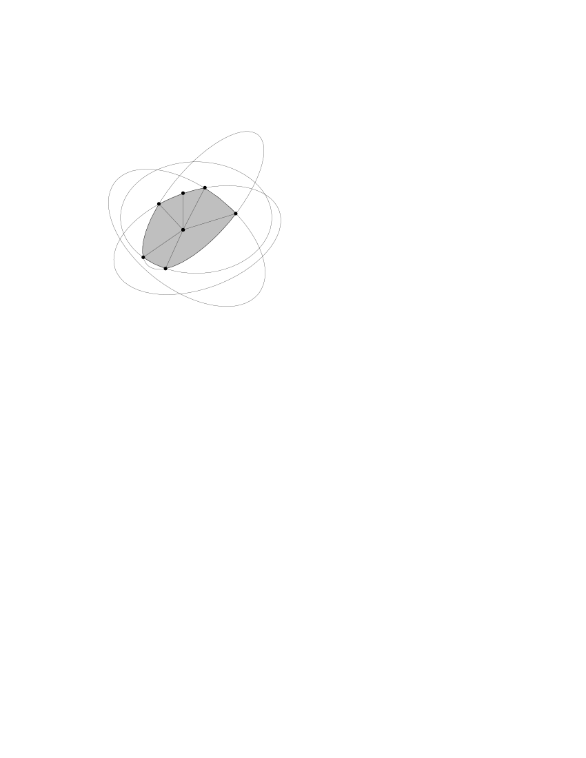
Figure 3: Arcs defining an intersection of ellipses.

Lemma 4.23.

If $\Delta_{c}\geq\Gamma$ for a constant $\Gamma>3$, then the region $R$ is the intersection of $O(n)$ ellipses, which may be identified in $O(n\log n)$ time.

Proof 4.24.

Let $a$ and $b$ be the foci of an ellipse contributing to the boundary of $R$ and containing the boundary point $c^{\prime}$; then $\Delta_{c}=\Delta_{c^{\prime}}=\Delta_{c^{\prime}}(a,b)$. By Lemma 2.4, $b$ must be one of the $k$ nearest neighbors of $a$. Therefore, the only ellipses that contribute to the boundary of $R$ are those found by reporting the $k$ nearest neighbors of each input point.

Lemma 4.25.

If $\Delta_{c}\leq\Gamma$ for a constant $\Gamma$, then the region $R$ is the intersection of $O(n)$ ellipses, which may be identified in $O(n\log n)$ expected time.

Proof 4.26.

As in Lemma 4.23, we will use the algorithm presented in Section 2 to identify the relevant ellipses. However the algorithm presented in Subsection 2.2 expects a center $c$ as input, and we are now computing $c$ as output. We overcome this obstacle by computing $c_{OPT}$, the solution to the unconstrained optimization problem discussed in Section 3. We then use the approach of Subsection 2.2, simulating the annuli centered on $c$ with the annuli centered on $c_{OPT}$. We will argue that for any $a\in V$ we can use techniques similar to those in Subsection 2.2 to identify $O(1)$ points, such that $\hat{a}$ is one of those points. Let $x=|cc_{OPT}|$; then $\hat{a}$ may fall into one of three categories. It may be roughly $x$ away from $c_{OPT}$, or closer, or farther.

Let $a\in V$, and suppose $\rho^{-1}x\leq|ac_{OPT}|\leq\rho x$. Then $a$ can only lie in one of two annuli centered on $c_{OPT}$, i.e. $A_{c_{OPT},i}$ or $A_{c_{OPT},i+1}$, for $i=\lfloor\log_{\rho}x\rfloor$; so for any $a$ we may pessimistically include all the $O(1)$ points in those annuli in the list of $\hat{a}$ candidates.

Suppose $|ac_{OPT}|>x$; then shifting the annuli’s center from $c$ to $c_{OPT}$ will cause $a$ to cross at most one annulus’ border. So if $a\in A_{c,i}$ then $a\in A_{c_{OPT},i-1}\cup A_{c_{OPT},i}\cup A_{c_{OPT},i+1}$. So for these points we include the points within $2l$ ranks of $a$ in $V_{S}$, rather than $l$ ranks as in Subsection 2.2.

Finally we consider points $a$ such that $|ac_{OPT}|<x$. By the assumption that $\Delta_{c_{OPT}}\leq\Gamma$ there can only be $O(1)$ such points; so we can pessimistically include all $O(1)$ such points.

So for each $a\in V$, we form the ellipses corresponding to $a$ paired with the points in the two annuli whose radii are close to $x$; the points appearing within $2l$ ranks of $a$ in the sorted sequence $V_{S}$; and the $O(1)$ points within $x$ of $c_{OPT}$.

Definition 4.27.

An arc ring is a pair $(r,S)$ describing the convex region inside the intersection of ellipses. $r$ is an arbitrary point inside the region. $S=\langle(e_{1},\theta_{1}),(e_{2},\theta_{2}),\ldots\rangle$ is a sequence of arcs, with each element $(e_{i},\theta_{i})$ describing a range of angles $\theta_{i-1}\leq\theta\leq\theta_{i}$ about $r$, for which the ellipse $e_{i}$ defines the boundary of the region (where $\theta_{0}\equiv\theta_{|S|}$). We require that the angle boundaries $\theta_{i}$ appear in ascending order, $\theta_{1}=0$, and $\theta_{|S|}=2\pi$.

Lemma 4.28.

There exists an arc ring describing any $R$ using $O(n\,2^{\alpha(n)})$ arcs.

Proof 4.29.

Lemmas 4.23 and 4.25 show that for any value of $\Delta_{c}$, $R$ may be described as the intersection of $O(n)$ ellipses. As shown in [9], a description of the intersection of $O(n)$ ellipses forms a Davenport-Schinzel sequence of order four; such a sequence has length $O(n\,2^{\alpha(n)})$. Hence $|S|\in O(n\,2^{\alpha(n)})$.

Lemma 4.30.

An arc ring $E$ describing $R$ may be generated in $O(n\,2^{\alpha(n)}\log n)$ time and queried in $O(\log n)$ time.

Proof 4.31.

$E$ may be formed in $O(n\,2^{\alpha(n)}\log n)$ time using a simple divide-and-conquer algorithm resembling merge sort. First partition the set of ellipses into two subsets of equal size, and compute the intersections $S_{1}$ and $S_{2}$ of the subsequences recursively. Then merge $S_{1}$ and $S_{2}$, as in merge sort, by comparing the least elements of each subsequence, $s_{1}$ and $s_{2}$ respectively, computing an element to append to $S=S_{1}\cup S_{2}$, and modifying or deleting $s_{1}$ and $s_{2}$. This may be done by partitioning the element with a greater angular interval into two elements, so that $s_{1}$ and $s_{2}$ cover exactly the same interval. If $s_{1}$ and $s_{2}$ do not intersect over that interval, then append whichever element is closer to $r$ to $S$; otherwise, append two elements corresponding to the closest ellipse on either side of the intersection point. The running time of this algorithm is given by the recurrence

$$T(|S|)=2T(|S|/2)+O(|S|)\enspace,$$

which solves to $T(n)\in O(|S|\log|S|)$; so the running time is $O(n\,2^{\alpha(n)}\log(n\,2^{\alpha(n)}))=O(n\,2^{\alpha(n)}\log n)$. Once $E$ has been constructed, it is possible to determine whether a point $a$ lies in $R$ by computing the angle between $r$ and $a$, then performing a binary search in $S$ to find the pertinent arc, and computing whether $a$ lies inside or outside that arc. This operation takes $O(\log n)$ time.

Theorem 4.32.

The optimal center $c\in V$ may be found in $O(n\,2^{\alpha(n)}\log^{2}n)$ expected time.

Proof 4.33.

The expected number of iterations of the outer loop of $CONSTRAINED-DILATION$ is $\log n$. The running time of each iteration is dominated by the construction of $R$, which can be achieved in $O(n\,2^{\alpha(n)}\log n)$ time. Hence the algorithm runs in $O(n\,2^{\alpha(n)}\log^{2}n)$ expected time.

References

- [1] P. K. Agarwal, R. Klein, C. Knauer, and M. Sharir. Computing the detour of polygonal curves. Technical Report B 02-03, Freie Universität Berlin, Fachbereich Mathematik und Informatik, 2002.
- [2] A. B. Amenta, M. W. Bern, and D. Eppstein. Optimal point placement for mesh smoothing. J. Algorithms, 30(2):302–322, February 1999. Special issue for 8th SODA.
- [3] T. M. Chan. An optimal randomized algorithm for maximum Tukey depth. In Proceedings of the fifteenth annual ACM-SIAM symposium on Discrete algorithms, pages 430–436. Society for Industrial and Applied Mathematics, 2004.
- [4] Z. Drezner and H. W. Hamacher. Facility Location: Applications and Theory. Springer-Verlag, 2001.
- [5] D. Eppstein. Spanning trees and spanners. In J.-R. Sack and J. Urrutia, editors, Handbook of Computational Geometry, chapter 9, pages 425–461. Elsevier, 2000.
- [6] D. Eppstein. Quasiconvex programming. ACM Computing Research Repository, cs.CG/0412046, 2004.
- [7] S. Langerman, P. Morin, and M. A. Soss. Computing the maximum detour and spanning ratio of planar paths, trees, and cycles. In Proceedings of the 19th Annual Symposium on Theoretical Aspects of Computer Science, pages 250–261. Springer-Verlag, 2002.
- [8] G. Narasimhan and M. Smid. Approximating the stretch factor of euclidean graphs. SIAM J. Comput., 30(3):978–989, 2000.
- [9] M. Sharir and P. K. Agarwal. Davenport-Schinzel sequences and their geometric applications. Cambridge University Press, 1996.
- [10] P. M. Vaidya. An algorithm for the all-nearest-neighbors problem. Discrete Comput. Geom., 4(2):101–115, 1989.