Exploring networks with traceroute-like probes: theory and simulations

Abstract

Mapping the Internet generally consists in sampling the network from a limited set of sources by using traceroute-like probes. This methodology, akin to the merging of different spanning trees to a set of destination, has been argued to introduce uncontrolled sampling biases that might produce statistical properties of the sampled graph which sharply differ from the original ones[1, 2, 3]. In this paper we explore these biases and provide a statistical analysis of their origin. We derive an analytical approximation for the probability of edge and vertex detection that exploits the role of the number of sources and targets and allows us to relate the global topological properties of the underlying network with the statistical accuracy of the sampled graph. In particular, we find that the edge and vertex detection probability depends on the betweenness centrality of each element. This allows us to show that shortest path routed sampling provides a better characterization of underlying graphs with broad distributions of connectivity. We complement the analytical discussion with a throughout numerical investigation of simulated mapping strategies in network models with different topologies. We show that sampled graphs provide a fair qualitative characterization of the statistical properties of the original networks in a fair range of different strategies and exploration parameters. Moreover, we characterize the level of redundancy and completeness of the exploration process as a function of the topological properties of the network. Finally, we study numerically how the fraction of vertices and edges discovered in the sampled graph depends on the particular deployements of probing sources. The results might hint the steps toward more efficient mapping strategies.

, , , ,

1 Introduction

A significant research and technical challenge in the study of large information networks is related to the lack of highly accurate maps providing information on their basic topology. This is mainly due to the dynamical nature of their structure and to the lack of any centralized control resulting in a self-organized growth and evolution of these systems. A prototypical example of this situation is faced in the case of the physical Internet. The topology of the Internet can be investigated at different granularity levels such as the router and Autonomous System (AS) level, with the final aim of obtaining an abstract representation where the set of routers (ASs) and their physical connections (peering relations) are the vertices and edges of a graph, respectively. In the absence of accurate maps, researchers rely on a general strategy that consists in acquiring local views of the network from several vantage points and merging these views in order to get a presumably accurate global map. Local views are obtained by evaluating a certain number of paths to different destinations by using specific tools such as traceroute or by the analysis of BGP tables. At first approximation these processes amount to the collection of shortest paths from a source vertex to a set of target vertices, obtaining a partial spanning tree of the network. The merging of several of these views provides the map of the Internet from which the statistical properties of the network are evaluated.

By using this strategy, a number of research groups have generated maps of the Internet [4, 5, 6, 7, 8], that have been used for the statistical characterization of the network properties. Defining $\mathcal{G}=(V,E)$ as the sampled graph of the Internet with $N=|V|$ vertices and $|E|$ edges, it is quite intuitive that the Internet is a sparse graph in which the number of edges is much lower than in a complete graph; i.e. $|E|\ll N(N-1)/2$. Equally important is the fact that the average distance, measured as the shortest path, between vertices is very small. This is the so called small-world property, that is essential for the efficient functioning of the network. Most surprising is the evidence of a skewed and heavy-tailed behavior for the probability that any vertex in the graph has degree $k$ defined as the number of edges linking each vertex to its neighbors. In particular, in several instances, the degree distribution appears to be approximated by $P(k)\sim k^{-\gamma}$ with $2\leq\gamma\leq 2.5$ [9]. Evidence for the heavy-tailed behavior of the degree distribution has been collected in several other studies at the router and AS level [10, 11, 12, 13, 14] and have generated a large activity in the field of network modeling and characterization [15, 16, 17, 18, 19].

While traceroute-driven strategies are very flexible and can be feasible for extensive use, the obtained maps are undoubtedly incomplete. Along with technical problems such as the instability of paths between routers and interface resolutions [20], typical mapping projects are run from relatively small sets of sources whose combined views are missing a considerable number of edges and vertices [14, 21]. In particular, the various spanning trees are specially missing the lateral connectivity of targets and sample more frequently vertices and links which are closer to each source, introducing spurious effects that might seriously compromise the statistical accuracy of the sampled graph. These sampling biases have been explored in numerical experiments of synthetic graphs generated by different algorithms[1, 2, 3]. Very interestingly, it has been shown that apparent degree distributions with heavy-tails may be observed even from homogeneous topologies such as in the classic Erdös-Rényi graph model[1, 2]. These studies thus point out that the evidence obtained from the analysis of the Internet sampled graphs might be insufficient to draw conclusions on the topology of the actual Internet network.

In this work we tackle this problem by performing a mean-field statistical analysis and extensive numerical study of shortest path routed sampling, considered as the first approximation to traceroute-sampling (see section 3), in different networks models. We derive in section 4 an approximate expression for the probability of edges and vertices to be detected that exploits the dependence upon the number of sources, targets and the topological properties of the networks. The expression shows the dependency of the efficiency of the mapping process upon the number of sources, targets and the topological properties of the network. Moreover, the analytical study provides a general understanding of which kind of topologies yields the most accurate sampling. In particular, we show that the map accuracy depends on the underlying network betweenness centrality distribution; the heavier the tail the higher the statistical accuracy of the sampled graph.

We substantiate our analytical finding with a throughout exploration of maps obtained varying the number of source-target pairs on networks models with different topological properties. In particular, we consider networks with degree distribution with poissonian, Weibull and power-law behavior (see section 5). According to the theoretical analysis, both the total number of probes deployed and the topological properties seem to play a primary role in the understanding of the level of the efficiency reached by the mapping process. As a measure of the efficiency of the mapping in different network topologies, we study the fractions of discovered vertices and edges as a function of the degree (section 6), stressing the agreement with the theoretical predictions. Other interesting quantities such as transit frequency and traffic entropy, are introduced in the study of the discovery process, with the aim of providing a complete framework for the study of sampling redundancy (section 7). Furthermore we focus on the study of the degree distributions obtained in the sampled graph and their resemblance to the original ones (see Section 8). Our results show that single source mapping processes face serious limitations in that also the targeting of the whole network results in a very partial discovery of its connectivity. On the contrary, the use of multiple sources promptly leads to obtained maps fairly consistent with the original sample, where the statistical degree distributions are qualitatively discriminated also at relatively low values of target density. A detailed discussion of the behavior of the degree distribution as a function of targets and sources is provided for sampled graphs with different topologies and compared with the insight obtained by analytical means.

In section 9, we also inspect quantitatively the portion of discovered network in different mapping strategies for the deployment of sources that however impose the same density of probes to the network; i.e. having the same probing load. We find the presence of a region of low efficiency (less vertices and edges discovered) depending on the relative proportion of sources and targets. This low efficiency region however corresponds to the optimal estimation of the network average degree. This finding calls for a “trade-off” between the accuracy in the observation of different quantities and hints to possible optimization procedures in the traceroute-driven mapping of large networks.

2 Related work

In this section, we shortly review some recent works devoted to the sampling of graphs by shortest path probing procedures. Lakhina et al. [1] have shown that biases can seriously affect the estimation of degree distributions. In particular, power-law like distributions can be observed for subgraphs of Erdös-Rényi random graphs when the subgraph is the product of a traceroute exploration with relatively few sources and destinations. They discuss the origin of these biases and the effect of the distance between source and target in the mapping process. In a recent work [2], Clauset and Moore have given analytical foundations to the numerical work of Lakhina et al. [1]. They have modeled the single source probing to all possible destinations using differential equations. For an Erdös-Renyi random graph with average degree $\overline{k}$, they have found that the connectivity distribution of the obtained spanning tree displays a power-law behavior $k^{-1}$, with an exponential cut-off setting in at a characteristic degree $k_{c}\sim\overline{k}$.

In a slightly different context, Petermann and De Los Rios have studied a traceroute-like procedure on various examples of scale-free graphs [3], showing that, in the case of a single source, power-law distributions with underestimated exponents are obtained. Analytical estimates of the measured exponents as a function of the true ones were also derived. Finally, a recent preprint by Guillaume and Latapy [23] reports about the shortest-paths explorations of synthetic graphs, focusing on the comparison between properties of the resulting sampled graph with those of the original network. The proportion of discovered vertices and edges in the graph as a function of the number of sources and targets gives also hints for an optimization of the exploration process.

All these pieces of work make clear the relevance of determining up to which extent the topological properties observed in sampled graphs are representative of that of the real networks.

3 A theoretical model for traceroute-like processes

In a typical traceroute study, a set of active sources deployed in the network sends traceroute probes to a set of destination vertices. Each probe collects information on all the vertices and edges traversed along the path connecting the source to the destination, allowing the discovery of the network [20]. By merging the information collected on each path it is then possible to reconstruct a partial map of the network (Fig.1). More in detail, the edges and the vertices discovered by each probe will depend on the “path selection criterium” used to decide the path between a pair of vertices. In the real Internet, many factors, including commercial agreement, traffic congestion and administrative routing policies, contribute to determine the actual path, causing it to differ even considerably from the shortest path. Despite these local, often unpredictable path distortions or inflations, a reasonable first approximation of the route traversed by traceroute-like probes is the shortest path between the two vertices. This assumption, however, is not sufficient for a proper definition of a traceroute model in that equivalent shortest paths between two vertices may exist. In the presence of a degeneracy of shortest paths we must therefore specify the path selection criterium by providing a resolution algorithm for the selection of shortest paths.

Figure 1: Illustration of the traceroute-like procedure. Shortest paths between the set of sources and the set of destination targets are discovered (shown in full lines) while other edges are not found (dashed lines). Note that not all shortest paths are found since the “Unique Shortest Path” procedure is used.

For the sake of simplicity we can define three selection mechanisms defining different ideal-paths that may account for some of the features encountered in Internet discovery:

• Unique Shortest Path (USP) probe. In this case the shortest path route selected between a vertex $i$ and the destination target $T$ is always the same independently of the source $S$ (the path being initially chosen at random among all the equivalent ones).

• Random Shortest Path (RSP) probe. The shortest path between any source-destination pair is chosen randomly among the set of equivalent shortest paths. This might mimic different peering agreements that make independent the paths among couples of vertices.

• All Shortest Paths (ASP) probe. The selection criterium discovers all the equivalent shortest paths between source-destination pairs. This might happen in the case of probing repeated in time (long time exploration), so that back-up paths and equivalent paths are discovered in different runs.

We will generically call $\mathcal{M}$-path the path found using one of these measurement or path selection mechanism. Actual traceroute probes contain a mixture of the three mechanisms defined above. We do not attempt, however, to account for all the subtleties that real studies encounters, i.e. IP routing, BGP policies, interface resolutions and many others. In fact, in the real mapping process, many effective heuristic strategies are commonly applied to improve the reliability and the performances of the sampling. For instance, the interface resolution is well achieved by the iffinder algorithm proposed by Broido and Claffy [11]. However, we will see that the different path selection criteria (p.s.c.) have only little influence on the general picture emerging from our results. Moreover, the USP procedure clearly represents the worst case scenario since, among the three different methods, it yields the minimum number of discoveries. For this reason, if not otherwise specified, we will report the USP data to illustrate the general features of our synthetic exploration. The interest of this analysis resides properly in the choice of working in the most pessimistic case, being aware that path inflations should actually provide a more pervasive sampling of the real network.

More formally, the experimental setup for our simulated traceroute mapping is the following. Let $G=(V,E)$ be a sparse undirected graph with vertices (vertices) $V=\{1,2,\cdots,N\}$ and edges (links) $E$. Then let us define the sets of vertices $\mathcal{S}=\{i_{1},i_{2},\cdots,i_{N_{S}}\}$ and $\mathcal{T}=\{j_{1},j_{2},\cdots,j_{N_{T}}\}$ specifying the random placement of $N_{S}$ sources and $N_{T}$ destination targets. For each ensemble of source-target pairs $\Omega=\{\mathcal{S},\mathcal{T}\}$, we compute with our p.s.c. the paths connecting each source-target pair. The sampled graph $\mathcal{G}=(V^{*},E^{*})$ is defined as the set of vertices $V^{*}$ (with $N^{*}=|V^{*}|$) and edges $E^{*}$ induced by considering the union of all the $\mathcal{M}$-paths connecting the source-target pairs. The sampled graph is thus analogous to the maps obtained from real traceroute sampling of the Internet.

In our study the parameters of interest are the density $\rho_{T}=N_{T}/N$ and $\rho_{S}=N_{S}/N$ of targets and sources. In general, traceroute-driven studies run from a relatively small number of sources to a much larger set of destinations. For this reason, in many cases it is appropriate to work with the density of targets $\rho_{T}$ while still considering $N_{S}$ instead of the corresponding density. Indeed, it is clear that while $100$ targets may represent a fair probing of a network composed by $500$ vertices, this number would be clearly inadequate in a network of $10^{6}$ vertices. On the contrary, the density of targets $\rho_{T}$ allows us to compare mapping processes on networks with different sizes by defining an intrinsic percentage of targeted vertices. In many cases, as we will see in the next sections, an appropriate quantity representing the level of sampling of the networks is $\epsilon=\frac{N_{S}N_{T}}{N}$, that measures the density of probes imposed to the system. In real situations it represents the density of traceroute probes in the network and therefore a measure of the load provided to the network by the measuring infrastructure.

In the following, our aim is to evaluate to which extent the statistical properties of the sampled graph $\mathcal{G}$ depend on the parameters of our experimental setup and are representative of the properties of the underlying graph $G$.

4 Mean-field theory of simulated mapping process

We begin our study by presenting a mean-field statistical analysis of the simulated traceroute mapping. Our aim is to provide a statistical estimate for the probability of edge and vertex detection as a function of $N_{S}$, $N_{T}$ and the topology of the underlying graph.

Let us define the quantity $\sigma_{i,j}^{(l,m)}$ that takes the value $1$ if the edge $(i,j)$ belongs to the selected $\mathcal{M}$-path between vertices $l$ and $m$, and $0$ otherwise. The indicator function that a given edge $(i,j)$ will be discovered and belongs to the sampled graph is given by

$$\pi_{i,j}=1-\prod_{l\neq m}\left(1-\sum_{s=1}^{N_{S}}\delta_{l,i_{s}}\sum_{t=1}^{N_{T}}\delta_{m,j_{t}}\sigma_{i,j}^{(l,m)}\right),$$ (1)

where $\delta_{i,j}$ is the Kronecker symbol and selects only vertices belonging to the set of sources or targets. In the case of a given set $\Omega=\{\mathcal{S},\mathcal{T}\}$, the above function is simply $\pi_{i,j}=1$ if the edge $(i,j)$ belongs to at least one of the $\mathcal{M}$-paths connecting the source-target pairs, and $0$ otherwise. While the above exact expression does not lead us too far in the understanding of the discovery probabilities, it is interesting to look at the process on a statistical ground by studying the average over all possible realizations of the set $\Omega=\{\mathcal{S},\mathcal{T}\}$. By definition we have that

$$\left\langle\sum_{t=1}^{N_{T}}\delta_{i,j_{t}}\right\rangle=\rho_{T}~{}~{}~{}\mbox{and}~{}~{}\left\langle\sum_{s=1}^{N_{S}}\delta_{i,i_{s}}\right\rangle=\rho_{S},$$ (2)

where $\left\langle\cdots\right\rangle$ identifies the average over all possible deployment of sources and targets $\Omega$. These equalities simply state that each vertex $i$ has, on average, a probability to be a source or a target that is proportional to their respective densities. In the following, we will make use of an uncorrelation assumption that yields an explicit approximation for the discovery probability. The assumption consists in neglecting correlations originated by the position of sources and targets on the discovery probability by different paths. While this assumption does not provide an exact treatment for the problem it generally conveys a qualitative understanding of the statistical properties of the system. In this approximation, the average discovery probability of an edge is

$$\left\langle\pi_{i,j}\right\rangle=1-\left\langle\prod_{l\neq m}\left(1-\sum_{s=1}^{N_{S}}\delta_{l,i_{s}}\sum_{t=1}^{N_{T}}\delta_{m,j_{t}}\sigma_{i,j}^{(l,m)}\right)\right\rangle$$

$$~{}~{}~{}~{}~{}~{}~{}~{}~{}~{}\simeq 1-\prod_{l\neq m}\left(1-\rho_{T}\rho_{S}\left\langle\sigma_{i,j}^{(l,m)}\right\rangle\right),$$ (3)

where in the last term we take advantage of neglecting correlations by replacing the average of the product of variables with the product of the averages and using Eq. (2). This expression simply states that each possible source-target pair weights in the average with the product of the probability that the end vertices are a source and a target; the discovery probability is thus obtained by considering the edge in an average effective media (mean-field) of sources and targets homogeneously distributed in the network. This approach is indeed akin to mean-field methods customarily used in the study of many particle systems where each particle is considered in an effective average medium defined by the uncorrelated averages of quantities. The realization average of $\left\langle\sigma_{i,j}^{(l,m)}\right\rangle$ is very simple in the uncorrelated picture, depending only of the kind of the probing model. In the case of the ASP probing, $\left\langle\sigma_{i,j}^{(l,m)}\right\rangle$ is just one if $(i,j)$ belongs to one of the shortest paths between $l$ and $m$, and $0$ otherwise. In the case of the USP and the RSP, on the contrary, only one path among all the equivalent ones is chosen. If we denote by $\sigma^{(l,m)}$ the number of shortest paths between vertices $l$ and $m$, and by $x_{i,j}^{(l,m)}$ the number of these paths passing through the edge $(i,j)$, the probability that the traceroute model chooses a path going through the edge $(i,j)$ between $l$ and $m$ is $\left\langle\sigma_{i,j}^{(l,m)}\right\rangle$ = $x^{(l,m)}_{i,j}/\sigma^{(l,m)}$.

The standard situation we consider is the one in which $\rho_{T}\rho_{S}\ll 1$ and since $\left\langle\sigma_{i,j}^{(l,m)}\right\rangle\leq 1$, we have

$$\prod_{l\neq m}\left(1-\rho_{T}\rho_{S}\left\langle\sigma_{i,j}^{(l,m)}\right\rangle\right)\simeq\prod_{l\neq m}\exp\left(-\rho_{T}\rho_{S}\left\langle\sigma_{i,j}^{(l,m)}\right\rangle\right),$$ (4)

that inserted in Eq.(3) yields

$$\left\langle\pi_{i,j}\right\rangle\simeq 1-\prod_{l\neq m}\left(\exp\left(-\rho_{T}\rho_{S}\left\langle\sigma_{i,j}^{(l,m)}\right\rangle\right)\right)=1-\exp\left(-\rho_{T}\rho_{S}b_{ij}\right),$$

where $b_{ij}=\sum_{l\neq m}\left\langle\sigma_{i,j}^{(l,m)}\right\rangle$. In the case of the USP and RSP probing, the quantity $b_{ij}$ is by definition the edge betweenness centrality $\sum_{l\neq m}x^{(l,m)}_{i,j}/\sigma^{(l,m)}$ [24, 25], sometimes also refereed to as “load” [26] (In the case of ASP probing, it is a closely related quantity). Indeed the vertex or edge betweenness is defined as the total number of shortest paths among pairs of vertices in the network that pass through a vertex or an edge, respectively. If there are multiple shortest paths between a pair of vertices, the path contributes to the betweenness with the corresponding relative weight. The betweenness gives a measure of the amount of all-to-all traffic that goes through an edge or vertex, if the shortest path is used as the metric defining the optimal path between pairs of vertices, and it can be considered as a non-local measure of the centrality of an edge or vertex in the graph.

The edge betweenness assumes values between $2$ and $N(N-1)$ and the discovery probability of the edge will therefore depend strongly on its betweenness. In particular, for edges with minimum betweenness $b_{ij}=2$ we have $\left\langle\pi_{i,j}\right\rangle\simeq 2\rho_{T}\rho_{S}$, that recovers the probability that the two end vertices of the edge are chosen as source and target. This implies that if the densities of sources and targets are small but finite in the limit of very large $N$, all the edges in the underlying graph have an appreciable probability to be discovered. Moreover, for edges with high betweenness the discovery probability approaches one. A fair sampling of the network is thus expected.

In most realistic samplings, however, we face a very different situation. While it is reasonable to consider $\rho_{T}$ a small but finite value, the number of sources is not extensive ($N_{S}\sim\mathcal{O}(1)$) and their density tends to zero as $N^{-1}$. In this case it is more convenient to express the edge discovery probability as

$$\left\langle\pi_{i,j}\right\rangle\simeq 1-\exp\left(-\epsilon\widetilde{b_{ij}}\right),$$ (5)

where $\epsilon=\rho_{T}N_{S}$ is the density of probes imposed to the system and the rescaled betweenness $\widetilde{b_{ij}}=N^{-1}b_{ij}$ is now limited in the interval $[2N^{-1},N-1]$. In the limit of large networks $N\to\infty$ it is clear that edges with low betweenness have $\left\langle\pi_{i,j}\right\rangle\sim\mathcal{O}(N^{-1})$, for any finite value of $\epsilon$. This readily implies that in real situations the discovery process is generally not complete, a large part of low betweenness edges being not discovered, and that the network sampling is made progressively more accurate by increasing the density of probes $\epsilon$.

A similar analysis can be performed for the discovery probability $\pi_{i}$ of a vertex $i$. For each source-target set $\Omega$ we have that

$$\pi_{i}=1-\left(1-\sum_{s=1}^{N_{S}}\delta_{i,i_{s}}-\sum_{t=1}^{N_{T}}\delta_{i,j_{t}}\right)\prod_{l\neq m\neq i}\left(1-\sum_{s=1}^{N_{S}}\delta_{l,i_{s}}\sum_{t=1}^{N_{T}}\delta_{m,j_{t}}\sigma_{i}^{(l,m)}\right).$$ (6)

where $\sigma_{i}^{(l,m)}=1$ if the vertex $i$ belongs to the $\mathcal{M}$-path between vertices $l$ and $m$, and $0$ otherwise. This time it has been considered that each vertex is discovered with probability one also if it is in the set of sources and targets. The second term on the right hand side therefore expresses the fact that the vertex $i$ does not belong to the set of sources and targets and it is not discovered by any $\mathcal{M}$-path between source-target pairs. By using the same mean-field approximation as previously, the average vertex discovery probability reads as

$$\left\langle\pi_{i}\right\rangle\simeq 1-(1-\rho_{S}-\rho_{T})\prod_{l\neq m\neq i}\left(1-\rho_{T}\rho_{S}\left\langle\sigma_{i}^{(l,m)}\right\rangle\right).$$ (7)

As for the case of the edge discovery probability, the average considers all possible source-target pairs weighted with probability $\rho_{T}\rho_{S}$. In the ASP model, the average $\left\langle\sigma_{i}^{(l,m)}\right\rangle$ is $1$ if $i$ belongs to one of the shortest paths between $l$ and $m$, and $0$ otherwise. For the USP and RSP models, $\left\langle\sigma_{i}^{(l,m)}\right\rangle$ = $x^{(l,m)}_{i}/\sigma^{(l,m)}$ where $x^{(l,m)}_{i}$ is the number of shortest paths between $l$ and $m$ going through $i$. If $\rho_{T}\rho_{S}\ll 1$, by using the same approximations used for Eq.(4) we obtain

$$\left\langle\pi_{i}\right\rangle\simeq 1-(1-\rho_{S}-\rho_{T})\exp\left(-\rho_{T}\rho_{S}b_{i}\right),$$ (8)

where $b_{i}=\sum_{l\neq m\neq i}\left\langle\sigma_{i}^{(l,m)}\right\rangle$. For the USP and RSP cases, $b_{i}=\sum_{l\neq m\neq i}x^{(l,m)}_{i}/\sigma^{(l,m)}$ is the vertex betweenness centrality, that is limited in the interval $[0,N(N-1)]$ [24, 25, 26]. The betweenness value $b_{i}=0$ holds for the leafs of the graph, i.e. vertices with a single edge, for which we recover $\left\langle\pi_{i}\right\rangle\simeq\rho_{S}+\rho_{T}$. Indeed, this kind of vertices are dangling ends discovered only if they are either a source or target themselves.

As discussed before, the most usual setup corresponds to a density $\rho_{S}\sim\mathcal{O}(N^{-1})$ and in the large $N$ limit we can conveniently write

$$\left\langle\pi_{i}\right\rangle\simeq 1-(1-\rho_{T})\exp\left(-\epsilon\widetilde{b_{i}}\right),$$ (9)

where we have neglected terms of order $\mathcal{O}(N^{-1})$ and the rescaled betweenness $\widetilde{b_{i}}=N^{-1}b_{i}$ is now defined in the interval $[0,N-1]$. This expression points out that the probability of vertex discovery is favored by the deployment of a finite density of targets that defines its lower bound.

We can also provide a simple approximation for the effective average degree $\left\langle k_{i}^{*}\right\rangle$ of the vertex $i$ discovered by our sampling process. Each edge departing from the vertex will contribute proportionally to its discovery probability, yielding

$$\left\langle k_{i}^{*}\right\rangle=\sum_{j}\left(1-\exp\left(-\epsilon\widetilde{b_{ij}}\right)\right)\simeq\epsilon\sum_{j}\widetilde{b_{ij}}.$$ (10)

The final expression is obtained for edges with $\epsilon\widetilde{b_{ij}}\ll 1$. Since the sum over all neighbors of the edge betweenness is simply related to the vertex betweenness as $\sum_{j}{b_{ij}}=2(b_{i}+N-1)$, where the factor $2$ considers that each vertex path traverses two edges and the term $N-1$ accounts for all the edge paths for which the vertex is an endpoint, this finally yields

$$\left\langle k_{i}^{*}\right\rangle\simeq 2\epsilon+2\epsilon\widetilde{b_{i}}.$$ (11)

The present analysis shows that the measured quantities and statistical properties of the sampled graph strongly depend on the parameters of the experimental setup and the topology of the underlying graph. The latter dependence is exploited by the key role played by edge and vertex betweenness in the expressions characterizing the graph discovery. The betweenness is a nonlocal topological quantity whose properties change considerably depending on the kind of graph considered. This allows an intuitive understanding of the fact that graphs with diverse topological properties deliver different answer to sampling experiments.

5 Definition of the graph models

In order to investigate numerically the traceroute-like exploration process, we have deliberately chosen simple models endowed with very well-defined topological properties, so as to give a clear result on which kind of topologies are related to good sampling performances and vice-versa. Starting from this first investigation, further studies could deal with more realistic models as those created using Internet topology generators [16, 15].

Let us consider sparse undirected graphs denoted by $G=(V,E)$ where the topological properties of a graph are fully encoded in its adjacency matrix $a_{ij}$, whose elements are $1$ if the edge $(i,j)$ exists, and $0$ otherwise. In particular, we will consider two main classes of graphs: i) Homogeneous graphs in which the degree distribution $P(k)$ has small fluctuations and a well defined average degree; ii) Heterogeneous graphs for which $P(k)$ is a broad distribution with heavy-tail and large fluctuations. In this context, the homogeneity refers to the existence of a meaningful characteristic average degree that represents the typical value in the graph. For instance, in graphs with poissonian-like degree distribution a vast majority of vertices has degree close to the average value and deviations from the average are exponentially small in number. On the contrary, graphs with heavy-tailed degree distribution are characterized by a strong heterogeneity encoded in the presence of very large fluctuations and degree values varying over a wide range of magnitudes.

5.1 Models

The most widely known model for homogeneous graphs is given by the classical Erdös-Rényi (ER) model [22]: in such random graphs $G_{N,p}$ of $N$ vertices, each edge is present in $E$ independently with probability $p$. The expected number of edges is therefore $|E|=pN(N-1)/2$. In order to have sparse graphs one thus needs to have $p$ of order $1/N$, since the average degree is $p(N-1)$. Erdös-Rényi graphs are typical examples of homogeneous graphs, with degree distribution following a Poisson law. Since $G_{N,p}$ can consist of more than one connected component, we consider only the largest of these components.

In opposition to the previous case, heterogeneous graphs are characterized by connectivity distributions spanning various orders of magnitude, with a heavy-tail at large $k$. In the literature, different definitions of heavy-tailed like distributions exist. While we do not want to enter the detailed definition of heavy-tailed distribution we have considered two classes of such distributions: (i) scale-free or Pareto distributions of the form $P(k)\sim k^{-\gamma}$ (RSF), and (ii) Weibull distributions (WEI) $P(k)=(a/c)(k/c)^{a-1}\exp(-(k/c)^{a})$. The scale-free distribution has a diverging second moment and therefore virtually unbounded fluctuations, limited only by eventual size-cut-off. The Weibull distribution has a coefficient of variation larger than the one of exponential distributions but is not power-law tailed. This distribution is akin to power-law distribution truncated by an exponential cut-off which are often encountered in the analysis of scale-free systems in the real world. Indeed, a truncation of the power-law behavior is generally due to finite-size effects and other physical constraints. Both forms have been proposed as representing the topological properties of the Internet [11]. In both cases, we have generated the corresponding random graphs by using the algorithm proposed by Molloy and Reed [30]. It consists in assigning to the vertices of the graph a fixed sequence of degrees $\{{k}_{i}\}$,  $i=1,\dots,N$, chosen at random from the desired degree distribution $P(k)$, and with the additional constraint that the sum $\sum_{i}{k}_{i}$ must be even. Then, the vertices are connected by $\sum_{i}{k}_{i}/2$ edges, respecting the assigned degrees and avoiding self- and multiple-connections. The parameters used are $a=0.25$ and $c=0.6$ for the Weibull distribution, and $\gamma=2.3$ for the RSF case. The main properties of the various graphs are summarized in table 1. In all numerical studies we have used networks of $N=10^{4}$ vertices. It is noteworthy that the maximum value of the degree ($k_{max}$) is of the same order as the average for homogeneous graphs, but much larger for heterogenous ones.

Table 1: Main characteristics of the graphs used in the numerical exploration.

	ER	ER	RSF	Weibull
$N$	$10^{4}$	$10^{4}$	$10^{4}$	$10^{4}$
$|E|$	$10^{5}$	$5.10^{5}$	$22000$	$55000$
$\overline{k}$	$20$	$100$	$4.4$	$11$
$k_{max}$	$40$	$140$	$3500$	$2000$

5.2 Betweenness centrality

Since the topological properties governing the traceroute exploration is the betweenness centrality, it is worth reviewing its general properties in the case of the models considered here. In Fig. 2 we report the vertex betweenness cumulative distributions for the ER model as well as for the graphs with scale-free or Weibull distributions of connectivity.

In homogeneous networks, the vertex and edge betweennesses are as well homogeneous quantities and their distributions are peaked around their average values $\overline{b}$ and $\overline{b_{e}}$, respectively, spanning only a small range of variations. These values can thus be considered as typical values. Moreover, the betweenness is correlated with the degree, as shown by the study of the rescaled betweenness averaged over vertices of given degree $k$, $\overline{b(k)}$, which increases with $k$.

For heterogeneous models, the betweenness distribution is heavy-tailed, allowing for an appreciable fraction of vertices and edges with very high betweenness[31]. In particular, in scale-free graphs the site betweenness is related to the vertices degree as $\overline{b(k)}\sim k^{\beta}$, where $\beta$ is an exponent depending on the model [31]. Since in heavy-tailed degree distributions the allowed degree is varying over several orders of magnitude, the same occurs for the betweenness values, as shown in Fig. 2, and the tail of the distribution is broader the broader the connectivity distribution: larger values are consequently reached for the RSF case with $\gamma=2.3$ than for the Weibull case.

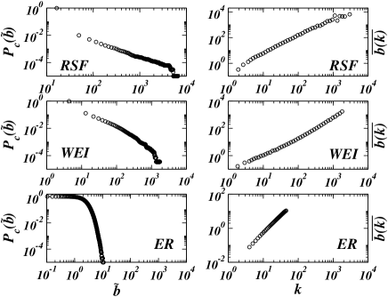
Figure 2: Cumulative distribution of the rescaled vertex betweenness (left) and average behavior as a function of the connectivity (right) in the graph models.

6 Efficiency in the sampling of graphs

Let us first consider the case of homogeneous graphs. Since a large majority of vertices and edges will have a betweenness very close to the average value, we can use Eq. (5) and (9) to estimate the order of magnitude of probes that allows a fair sampling of the graph. Indeed, both $\langle\pi_{i,j}\rangle$ and $\langle\pi_{i}\rangle$ tend to $1$ if $\epsilon\gg$ max$\left[\overline{b}^{-1},\overline{b_{e}}^{-1}\right]$. In this limit all edges and vertices will have probability to be discovered very close to one. At lower value of $\epsilon$, obtained by varying $\rho_{T}$ and $N_{S}$, the underlying graph is only partially discovered. Fig. 3 shows the behavior of the fraction $N_{k}^{*}/N_{k}$ of discovered vertices of degree $k$, where $N_{k}$ is the total number of vertices of degree $k$ in the underlying graph, and the fraction of discovered edges $\left\langle k^{*}\right\rangle/k$ in vertices of degree $k$. $N_{k}^{*}/N_{k}$ naturally increases with the density of targets and sources, and it is slightly increasing with $k$. The latter behavior can be easily understood by noticing that vertices with larger degree have on average a larger betweenness. On the other hand, the range of variation of $k$ in homogeneous graphs is very narrow and only a large level of probing may guarantee very large discovery probabilities. Similarly the behavior of the effective discovered degree can be understood by looking at Eq. (11). Indeed the initial decrease of $\left\langle k^{*}\right\rangle/k$ is finally compensated by the increase of $\overline{b(k)}$.

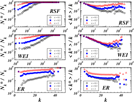
Figure 3: Frequency $N_{k}^{*}/N_{k}$ of detecting a vertex of degree $k$ (left) and proportion of discovered edges $\left\langle k^{*}\right\rangle/k$ (right) as a function of the degree in the RSF, WEI, and ER graph models. The exploration setup considers $N_{S}=2$ and increasing probing level $\epsilon$ obtained by progressively higher density of targets $\rho_{T}$. The axis of ordinates is in log scale to allow a finer resolution.

The situation is different in graphs with heavy-tailed connectivity distributions, for which the betweenness spans various orders of magnitude. In such a situation, even in the case of small $\epsilon$, vertices whose betweenness is large enough ($b_{i}\epsilon\gg 1$) have $\left\langle\pi_{i}\right\rangle\simeq 1$. Therefore all vertices with degree $k\gg\epsilon^{-1/\beta}$ will be detected with probability one. This is clearly visible in Fig. 3 where the discovery probability $N_{k}^{*}/N_{k}$ of vertices with degree $k$ saturates to one for large degree values. Consistently, the degree value at which the curve saturates decreases with increasing $\epsilon$. A similar effect is appearing in the measurements concerning $\left\langle k^{*}\right\rangle/k$. After an initial decay (Fig. 3) the effective discovered degree is increasing with the degree of the vertices. This qualitative feature is captured by Eq. (11) that gives $\left\langle k^{*}\right\rangle/k\simeq\epsilon k^{-1}(1+\overline{b(k)})$. At large $k$ the term $k^{-1}\overline{b(k)}\sim k^{\beta-1}$ takes over and the effective discovered degree approaches the real degree $k$. Moreover, it appears clearly that the broader the distribution of betweennesses or connectivities, the better the sampling obtained.

7 Redundancy and dissymmetry of the discovery process

In this section we introduce tools suitable to estimate how traceroute-like procedures discover the vertices and the edges of the unknown underlying network. The most common biases affecting the mapping process concern the miss of lateral connectivity, and the multiple sampling of central vertices (and edges), which may affect the efficiency of the whole process. While the first problem might be solved by an optimization in the deployment of probes, actually relying on a criterion of decentralization of sources and targets, multiple sampling can be studied through some general concepts like the redundancy and dissymmetry of the discovery process.

7.1 Redundancy

Let us define the edge redundancy $r_{e}(i,j)$ of an edge $(i,j)$ in a traceroute-sampling as the number of probes passing through the edge $(i,j)$. Using the notations of section 4, this quantity is written for a given set of probes and targets as

$$r_{e}(i,j)=\sum_{l\neq m}\left(\sum_{s=1}^{N_{S}}\delta_{l,i_{s}}\sum_{t=1}^{N_{T}}\delta_{m,i_{t}}\sigma_{i,j}^{(l,m)}\right).$$ (12)

Averaging over all possible realizations and assuming the uncorrelation hypothesis, we obtain

$$\left\langle r_{e}(i,j)\right\rangle=\simeq\sum_{l\neq m}\rho_{T}\rho_{S}\left\langle\sigma_{i,j}^{(l,m)}\right\rangle=\rho_{T}\rho_{S}b_{ij}\ .\ \ \ \ \ \$$ (13)

This result implies that the average redundancy of an edge is related to the density of sources and targets, but also to the edge betweenness. For example, an edge of minimum betweenness $b_{ij}=2$ can be discovered at most twice in the extreme limit of an all-to-all probing. On the contrary, a very central edge of betweenness $b_{ij}$ close to the maximum $N(N-1)$, would be discovered with a redundancy close to $(N-1)$ by a traceroute-probing from a single source to all the possible destinations.

Similarly, the redundancy $r_{n}(i)$ of a vertex $i$, intended as the number of times the probes cross the vertex $i$, can be obtained:

$$r_{n}(i)=\sum_{l\neq m}\sigma_{i}^{(l,m)}\sum_{s=1}^{N_{S}}\delta_{l,i_{s}}\sum_{t=1}^{N_{T}}\delta_{m,i_{t}}\ .$$ (14)

After separating the cases $l=i$ and $m=i$ in the sum, the averaging over the positions of sources and targets yields in the mean-field approximation:

$$\left\langle r_{n}(i)\right\rangle=\sum_{l\neq m\neq i}\rho_{S}\rho_{T}\langle\sigma_{i}^{(l,m)}\rangle+2\rho_{S}\rho_{T}N\simeq 2\epsilon+\rho_{S}\rho_{T}b_{i}\ .$$ (15)

In this case, a term related to the number of traceroute probes $\epsilon$ appears, showing that a part of the mapping effort unavoidably ends up in generating vertex detection redundancy.

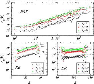
Figure 4: Average vertex redundancy as a function of the degree $k$ for RSF (top) and ER (bottom) model ($N=10^{4}$). For the ER model, two blocks of data are plotted, for $\overline{k}=20$ (left) and for $\overline{k}=100$ (right) The target density is fixed ($\rho_{T}=0.1$), and $N_{S}=2$ (circles), $10$ (squares), $20$ (triangles). The dashed lines represent the analytical prediction $2\epsilon+\rho_{S}\rho_{T}\overline{b(k)}$ in perfect agreement with the simulations.

In Fig. 4 we report the behavior of the average vertex redundancy as a function of the degree $k$ for both homogeneous and heterogeneous graphs. For both models, the behaviors are in good agreement with the mean-field prediction, showing the tight relation between redundancy and betweenness centrality.

In the case of heavy-tailed underlying networks, the vertex redundancy typically grows as a power-law of the degree, while the values for random graphs vary on a smaller scale. This behavior points out that the intrinsic hierarchical structure of scale-free networks plays a fundamental role even in the process of path routing, resulting in a huge number of probes iteratively passing through the same set of few hubs. On the other hand, for homogeneous graphs the total number of vertex discoveries is quite uniformly distributed on the whole range of connectivity, independently of the relative importance of the vertices.

7.2 Dissymmetry: Participation Ratio

The high rate of redundancy intrinsic to the exploration process, however, does not imply that the local topology close to a vertex is well discovered: preferential paths could indeed carry most of the probing effort leading to just a partial discovery of the vertex connections. This amounts to a dissymmetry of the exploration process that probes some edges much more than others, eventually ignoring some of those, in the neighborhood of a given vertex. Together with redundancy measures, let us consider the relative number of occurrences of a given edge $(i,j)$ during the traceroute, with respect to the total occurrence for the edges in the neighborhood of $i$. For each discovered vertex $i$, we can thus define a set of frequencies $\{f_{j}^{(i)}\}_{j\in\mathcal{V}(i)}$ for the edges $(i,j)$ of its neighborhood. In terms of redundancy the edge frequency $f_{j}^{(i)}$ is defined as

$$f_{j}^{(i)}=\frac{r_{e}(i,j)}{\sum_{j\in\mathcal{V}(i)}r_{e}(i,j)},\ \ \ \ 0\leq f_{j}^{(i)}\leq 1\ \ \forall(i,j)\in E,$$ (16)

and indicates the probability that any given probing path discovering the vertex $i$, is passing by the edge $(i,j)$.

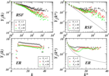
Figure 5: Participation Ratio as a function of real ($k$) and discovered ($k^{*}$) connectivity for RSF (top) and ER (bottom) models ($N=10^{4}$). The target density is fixed ($\rho_{T}=0.1$) and three value of $N_{S}$ are presented: 2 (circles), 10 (squares), 20 (triangles). The dashed lines correspond to the $1/k^{*}$ bound.

The dissymmetry of the discovery of the neighborhood of a vertex may be quantified through the participation ratio of these frequencies:

$$Y_{2}(i)=\sum_{j\in\mathcal{V}(i)}{\left(f_{j}^{(i)}\right)}^{2}\ .$$ (17)

If all the edge frequencies of $i$ are of the same order $\sim 1/{k^{*}_{i}}$ (only discovered links give a finite contribution), the participation ratio should decrease as $1/{k^{*}_{i}}$ with increasing discovered connectivity ${k^{*}_{i}}$. Hence, in the limit of an optimally symmetric sampling, it should yield a strict power law behavior $Y_{2}(k^{*})\sim{k^{*}}^{-1}$. On the contrary, when only few links are preferred, for instance because more central in the shortest path routing, the sum is dominated by these terms, leading to a value closer to the upper bound $1$. Numerical data for $Y_{2}$ as a function of the actual ($k$) and discovered ($k^{*}$) connectivity for different probing efforts, are displayed in Fig. 5. For heterogeneous graphs, the values of $Y_{2}$ tend towards the curve ${k^{*}}^{-1}$ for increasing $\epsilon$. In both cases this behavior is better achieved at high degree values. The tendency of high degree vertices to be better sampled in a more symmetrical way is evident in the diagram for $Y_{2}(k)$, where a crossover at large degrees appears. On the contrary, in the homogeneous case (ER), the figures show a general high level of dissymmetry persistent at all degree values, only slightly dependent on the actual connectivity and the probing effort.

7.3 Dissymmetry: Entropy Measure

In order to provide an alternative and in some cases more accurate study of the dissymmetry of the exploration process, we introduce a more refined frequency, $f_{kj}^{(i)}$ defined as the number of probes passing through the pair $(k,i)-(i,j)$ of edges centered on the vertex $i$. This is the probability of a probe to traverse a couple of edges with respect to the total number of transits through any of the possible couples of edges in the neighborhood of $i$. This frequency takes fully into account the path traversing each vertex and the dissymmetry of the flow. By means of this frequency, we define an entropy measure providing supplementary evidence of the tight relation between local accuracy, dissymmetry of sampling and topological characterization of graphs. Indeed, a traceroute discovering vertices crossing a larger variety of their links, and with different paths, is expected to be more accurate (and likely efficient) than the one always selecting the same path. In the same spirit of the Shannon entropy, which is a good indicator of disorder, we define the local traceroute entropy of a vertex $i$ by

$$h_{i}=-\frac{1}{\log{({k^{*}}_{i}(k^{*}_{i}-1))}}\sum_{k\neq j\in\mathcal{V}(i)}f_{kj}^{(i)}\log{f_{kj}^{(i)}},$$ (18)

where $\log{{k^{*}_{i}}}$ is simply a normalization factor. This quantity is bounded in the interval $0\leq h(i)\leq 1$. The case $h_{i}=1$ is reached when all the frequencies of probes spanning the edge couples of the vertex are equal. The case $H\simeq 0$ corresponds to a dominating frequency in a specific edge couple. Also in this case it is possible to study the degree spectrum $H(k)$ of the entropy by measuring the average entropy on vertices with given degree $k$.

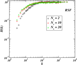
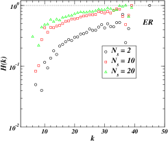
Figure 6: Entropy vs. $k$: a saturation effect is clear at medium-high degree vertices for scale free topologies (RSF), instead of a more regular increasing for homogeneous graphs (ER). In the figure there are different curves for $N_{S}$ = $2$ (circles), $10$ (squares), $20$ (triangles) and $\rho_{T}=0.1$.

The numerical data of $H(k)$ for RSF and ER models and for different levels of probing are reported in Fig. 6. The values for ER are slightly increasing both for increasing degree $k$ and number of sources $N_{S}$, with no qualitative difference in the behavior at low or high degree regions. On the other hand, the case of heterogeneous networks agrees with the previous observations. The curve for $H(k)$, indeed, shows a saturation phenomenon to values very close to the maximum $1$ at large enough degree, indicating a very symmetric sampling of these vertices.

In summary the previous studies indicates that in the case of heterogeneous networks, the hubs and high betweenness vertices are in general sampled redundantly, however, obtaining a rather symmetrical discovery of their neighborhood. On the contrary, homogeneous networks do not allow the presence of hubs and vertices are suffering a less redundant sampling while showing a high dissymmetry of the local exploration process. This results might be useful in deciding source-target deployment strategies, by taking into account the underlying topology of the network.

8 Degree distribution measurements

A very important quantity in the study of the statistical accuracy of the sampled graph is the degree distribution. Fig. 7 shows the cumulative degree distribution $P_{c}(k^{*}>k)$ of the sampled graph defined by the ER model for increasing density of targets and sources. Sampled distributions are only approximating the genuine distribution, however, for $N_{S}\geq 2$ they are far from true heavy-tail distributions at any appreciable level of probing. Indeed, the distribution runs generally over a small range of degrees, with a cut-off that sets in at the average degree $\overline{k}$ of the underlying graph. In order to stretch the distribution range, homogeneous graphs with very large average degree $\overline{k}$ must be considered; however, other distinctive spurious effects appear in this case. In particular, since the best sampling occurs around the high degree values, the distributions develop peaks that show in the cumulative distribution as plateaus (see Fig.8). Finally, in the case of RSP and ASP model, we observe that the obtained distributions are closer to the real one since they allow a larger number of discoveries.

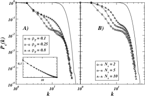
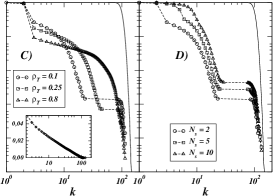
Figure 7: Cumulative degree distribution of the sampled ER graph for USP probes. Figures A) and B) correspond to $\overline{k}=20$, and C) and D) to $\overline{k}=100$. Figures A) and C) show sampled distributions obtained with $N_{S}=2$ and varying density target $\rho_{T}$. In the insets we report the peculiar case $N_{S}=1$ that provides an apparent power-law behavior with exponent $-1$ at all values of $\rho_{T}$, with a cut-off depending on $\overline{k}$. The insets are in lin-log scale to show the logarithmic behavior of the corresponding cumulative distribution. Figures B) and D) correspond to $\rho_{T}=0.1$ and varying number of sources $N_{S}$. The solid lines are the degree distributions of the underlying graph. For $\overline{k}=100$, the sampled cumulative distributions display plateaus corresponding to peaks in the degree distributions, induced by the sampling process.

Only in the peculiar case of $N_{S}=1$ an apparent scale-free behavior with slope $-1$ is observed for all target densities $\rho_{T}$, as analytically shown by Clauset and Moore [2]. Also in this case, the distribution cut-off is consistently determined by the average degree $\overline{k}$. It is worth noting that the experimental setup with a single source is a limit case corresponding to a highly asymmetric probing process; it is therefore badly, if at all, captured by our statistical analysis which assumes homogeneous deployment.

The present analysis shows that in order to obtain a sampled graph with apparent scale-free behavior on a degree range varying over $n$ orders of magnitude we would need the very peculiar sampling of a homogeneous underlying graph with an average degree $\overline{k}\simeq 10^{n}$; a rather unrealistic situation in the Internet and many other information systems where $n\geq 2$.

In section 6, we have shown clearly that, in heterogeneous graphs, vertices with high degree are efficiently sampled with an effective measured degree that is rather close to the real one. This means that the degree distribution tail is fairly well sampled while deviations should be expected at lower degree values. This is indeed what we observe in numerical experiments on graphs with heavy-tailed distributions (see Fig. 8). Despite both underlying graphs have a small average degree, the observed degree distribution spans more than two orders of magnitude. The distribution tail is fairly reproduced even at rather small values of $\epsilon$. The data shows clearly that the low degree regime is instead under-sampled. This undersampling can either yield an apparent change in the exponent of the degree distribution (as also noticed in [3] for single source experiments), or, if $N_{S}$ is small, yield a power-law like distribution for an underlying Weibull distribution. Furthermore, as Fig. 8 shows, an increase in the number of sources starts to discriminate between scale-free and Weibull distributions by detecting a curvature in the second case even at small values $\rho_{T}=0.25$. It is, however, fair to say that while the experiments clearly points out a broad and heavy-tailed distribution, the distinction between different types of heavy-tailed distribution needs an adequate level of probing.

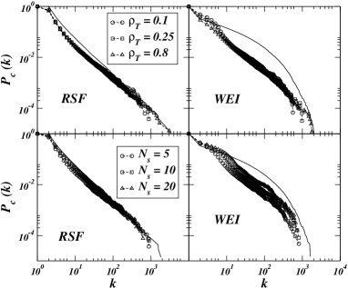
Figure 8: Cumulative degree distributions of the sampled RSF and WEI graphs for USP probes. The top figures show sampled distributions obtained with $N_{S}=5$ and varying density target $\rho_{T}$. The figures on the bottom correspond to $\rho_{T}=0.25$ and varying number of sources $N_{S}$. The solid lines are the degree distributions of the underlying graph.

In conclusion, graphs with heavy-tailed degree distribution allow a better qualitative representation of their statistical features in sampling experiments. Indeed, the most important properties of these graphs are related to the heavy-tail part of the statistical distributions that are indeed well discriminated by the traceroute-like exploration. On the other hand, the accurate identification of the distribution forms requires a fair level of sampling that it is not clear how to determine quantitatively in the case of an unknown underlying network. We will discuss the implications of these results in real Internet measurements in Sec. 10.

9 Optimization of mapping strategies

In the previous sections we have shown that it is possible to have a general qualitative understanding of the efficiency of network exploration and the induced biases on the statistical properties. The quantitative analysis of the sampling strategies, however, is a much harder task that calls for a detailed study of the discovered proportion of the underlying graph and the precise deployment of sources and targets. In this perspective, very important quantities are the fraction $N^{*}/N$ and $E^{*}/E$ of vertices and edges discovered in the sampled graph, respectively. Unfortunately, the mean-field approximation breaks down when we aim at a quantitative representation of the results. The neglected correlations are in fact very important for the precise estimate of the various quantities of interest. For this reason we performed an extensive set of numerical explorations aimed at a fine determination of the level of sampling achieved for different experimental setups.

In Fig. 9 we report the proportion of discovered edges in the numerical exploration of the graph models defined previously for increasing level of probing $\epsilon$. The level of probing is increased either by raising the number of sources at fixed target density or by raising the target density at fixed number of sources. As expected, both strategies are progressively more efficient with increasing levels of probing.

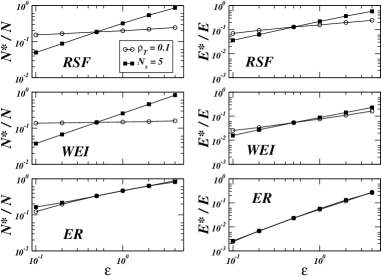
Figure 9: Behavior of the fraction of discovered edges in explorations with increasing $\epsilon$. For each underlying graph studied we report two curves corresponding to larger $\epsilon$ achieved by increasing the target density $\rho_{T}$ at constant $N_{S}=5$ (squares) or the number of sources $N_{S}$ at constant $\rho_{T}=0.1$ (circles).

In heterogeneous graphs, it is also possible to see that when the number of sources is $N_{S}\sim\mathcal{O}(1)$ the increase of the number of targets achieves better sampling than increasing the deployed sources. On the other hand, it is easy to perceive that the shortest path route mapping is a symmetric process if we exchange sources with targets. This is confirmed by numerical experiments in which we use a very large number of sources and a number of targets $\rho_{T}\sim\mathcal{O}(1/N)$, where the trends are opposite: the increase of the number of sources achieves better sampling than increasing the deployed targets.

This finding hints toward a behavior that is determined by the number of sources and targets, $N_{S}$ and $N_{T}$. Any quantity is thus a function of $N_{S}$ and $N_{T}$, or equivalently of $N_{S}$ and $\rho_{T}$. This point is clearly illustrated in Fig. 10, where we report the behavior of $E^{*}/E$ and $N^{*}/N$ at fixed $\epsilon$ and varying $N_{S}$ and $\rho_{T}$. The curves exhibit a non-trivial behavior and since we will work at fixed $\epsilon=\rho_{T}N_{S}$, any measured quantity can then be written as $f(\rho_{T},\epsilon/\rho_{T})=g_{\epsilon}(\rho_{T})$. Very interestingly, the curves show a structure allowing for local minima and maxima in the discovered portion of the underlying graph.

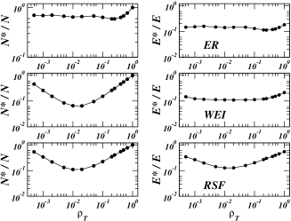
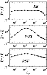
Figure 10: Behavior as a function of $\rho_{T}$ of the fraction of discovered edges and vertices in explorations with fixed $\epsilon$ (here $\epsilon=2$). Since $\epsilon=\rho_{T}N_{S}$, the increase of $\rho_{T}$ corresponds to a lowering of the number of sources $N_{S}$. The plots on the right show the fraction of the normalized average degree $\overline{k}^{*}/\overline{k}$.

This feature can be explained by a simple symmetry argument. The model for traceroute is symmetric by the exchange of sources and targets, which are the endpoints of shortest paths: an exploration with $(N_{T},N_{S})=(N_{1},N_{2})$ is equivalent to one with $(N_{T},N_{S})=(N_{2},N_{1})$. In other words, at fixed $\epsilon=N_{1}N_{2}/N$, a density of targets $\rho_{T}=N_{1}/N$ is equivalent to a density $\rho^{\prime}_{T}=N_{2}/N$. Since $N_{2}=\epsilon/\rho_{T}$ we obtain that at constant $\epsilon$, experiments with $\rho_{T}$ and $\rho^{\prime}_{T}=\epsilon/(N\rho_{T})$ are equivalent obtaining by symmetry that any measured quantity obeys the equality $g_{\epsilon}(\rho_{T})=g_{\epsilon}\left(\frac{\epsilon}{N\rho_{T}}\right)$. This relation implies a symmetry point signaling the presence of a maximum or a minimum at $\rho_{T}=\epsilon/(N\rho_{T})$. We therefore expect the occurrence of a symmetry in the graphs of Fig.10 at $\rho_{T}\simeq\sqrt{\epsilon/N}$. Indeed, the symmetry point is clearly visible and in quantitative good agreement with the previous estimate in the case of heterogeneous graphs. On the contrary, homogeneous underlying topology have a smooth behavior that makes difficult the clear identification of the symmetry point. Moreover, USP probes create a certain level of correlations in the exploration that tends to hide the complete symmetry of the curves.

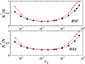
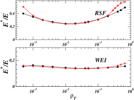
Figure 11: Behavior as a function of $\rho_{T}$ of the fraction of discovered edges and vertices in explorations with fixed $\epsilon$ (here $\epsilon=2$). The circles correspond to a random deployment of sources and targets while the crosses are obtained when sources and targets are vertices with lowest betweenness vertices.

The previous results imply that at fixed levels of probing $\epsilon$ different proportions of sources and targets may achieve different levels of sampling. This hints to the search for optimal strategies in the relative deployment of sources and targets. The picture, however, is more complicate if we look at other quantities in the sampled graph. In Fig.10 we show the behavior at fixed $\epsilon$ of the average degree $\overline{k}^{*}$ measured in sampled graphs normalized by the actual average degree $\overline{k}$ of the underlying graph as a function of $\rho_{T}$. The plot shows also in this case a symmetric structure. By comparing the data of Fig.10 we notice that the symmetry point is of a different nature for different quantities: the minimum in the fraction of discovered edges corresponds to the best estimate of the average degree. In other words, the best level of sampling is achieved at particular values of $\epsilon$ and $N_{S}$ that are conflicting with the best sampling of other quantities.

The evidence purported in this section hints to a possible optimization of the sampling strategy. The optimal solution, however, appears as a trade-off strategy between the different level of efficiency achieved in competing ranges of the experimental setup. In this respect, a detailed and quantitative investigation of the various quantities of interest in different experimental setups is needed in order to pinpoint the most efficient deployment of source-target pairs depending on the underlying graph topology. While such a detailed analysis lies beyond the scope of the present study, an interesting hint comes from the analytical results of section 4: since vertices with large betweenness have typically a very large probability of being discovered, placing the sources and targets preferentially on low-betweenness vertices (the most difficult to discover) may have an impact on the whole process. This is what we investigate in Fig. 11 in which we report the fraction of vertices and edges discovered by either a random deployment of sources and targets or a deployment on the lowest-betweenness vertices. It is apparent that such a deployment allows to discover larger parts of the network. Of course the procedure used is unrealistic since identifying low-betweenness vertices is not an easy task. The usual correlation between connectivity and betweenness however indicates that the exploration of a real network could be improved by a massive deployment of sources using low-connectivity vertices.

10 Conclusions and outlook

The rationalization of the exploration biases at the statistical level provides a general interpretative framework for the results obtained from the numerical experiments on graph models. The sampled graph clearly distinguishes the two situations defined by homogeneous and heavy-tailed topologies, respectively. This is due to the exploration process that statistically focuses on high betweenness vertices, thus providing a very accurate sampling of the distribution tail. In graphs with heavy-tails, such as scale-free networks, the main topological features are therefore easily discriminated since the relevant statistical information is encapsulated in the degree distribution tail which is fairly well captured. Quite surprisingly, the sampling of homogeneous graphs appears more cumbersome than those of heavy-tailed graphs. Dramatic effects such as the existence of apparent power-laws, however, are found only in very peculiar cases. In general, exploration strategies provide sampled distributions with enough signatures to distinguish at the statistical level between graphs with different topologies.

This evidence might be relevant in the discussion of real data from Internet mapping projects. Indeed, data available so far indicate the presence of heavy-tailed degree distribution both at the router and AS level. In the light of the present discussion, it is very unlikely that this feature is just an artifact of the mapping strategies. The upper degree cut-off at the router and AS level runs up to $10^{2}$ and $10^{3}$, respectively. A homogeneous graph should have an average degree comparable to the measured cut-off and this is hardly conceivable in a realistic perspective (for instance, it would require that nine routers over ten would have more than 100 links to other routers). In addition, the major part of mapping projects are multi-source, a feature that we have shown to readily wash out the presence of spurious power-law behavior. On the contrary, heterogeneous networks with heavy-tailed degree distributions are sampled with particular accuracy for the large degree part, generally at all probing levels. This makes very plausible, and a natural consequence, that the heavy-tail behavior observed in real mapping experiments is a genuine feature of the Internet. Furthermore, heterogeneous graphs show a striking tendency to improve the mapping efficiency at large degree vertices, while exponential graphs seem to respond in a homogeneous way independent of the degree value.

On the other hand, it is important to stress that while at the qualitative level the sampled graphs allow a discrimination of the statistical properties, at the quantitative level they might exhibit considerable deviations from the true values such as size, average degree, and the precise analytic form of the heavy-tailed degree distribution. For instance, the exponent of the power-law behavior appears to suffer from noticeable biases. In this respect, it is of major importance to define strategies that optimize the estimate of the various parameters and quantities of the underlying graph. In this paper we have shown that the proportion of sources and targets may have an impact on the accuracy of the measurements even if the number of total probes imposed to the system is the same. For instance, the deployment of a highly distributed infrastructure of sources probing a limited number of targets may result as efficient as few very powerful sources probing a large fraction of the addressable space [32]. The optimization of large network sampling is therefore an open problem that calls for further work aimed at a more quantitative assessment of the mapping strategies both on the analytic and numerical side.

References

- [1] A. Lakhina, J. W. Byers, M. Crovella and P. Xie, “Sampling Biases in IP Topology Measurements,” Technical Report BUCS-TR-2002-021, Department of Computer Sciences, Boston University (2002).
- [2] A. Clauset and C. Moore, “Why Mapping the Internet is Hard,” arXiv:cond-mat/0407339 (2004).
- [3] T. Petermann and P. De Los Rios, “Exploration of Scale-Free Networks - Do we measure the real exponents?,” Eur. Phys. J. B 201-204 (2004).
- [4] The National Laboratory for Applied Network Research (NLANR), sponsored by the National Science Foundation. (see http://moat.nlanr.net/).
- [5] The Cooperative Association for Internet Data Analysis (CAIDA), located at the San Diego Supercomputer Center. (see http://www.caida.org/home/).
- [6] Topology project, Electric Engineering and Computer Science Department, University of Michigan (http://topology.eecs.umich.edu/).
- [7] SCAN project at the Information Sciences Institute (http://www.isi.edu/div7/scan/).
- [8] Internet mapping project at Lucent Bell Labs (http://www.cs.bell-labs.com/who/ches/map/).
- [9] M. Faloutsos, P. Faloutsos, and C. Faloutsos, “On Power-law Relationships of the Internet Topology,” ACM SIGCOMM ’99, Comput. Commun. Rev. , 251–262 (1999).
- [10] R. Govindan and H. Tangmunarunkit, “Heuristics for Internet Map Discovery,” Proc. of IEEE Infocom 2000, Volume 3, IEEE Computer Society Press, 1371–1380, (2000).
- [11] A. Broido and K. C. Claffy, “Internet topology: connectivity of IP graphs,” San Diego Proceedings of SPIE International symposium on Convergence of IT and Communication. Denver, CO. 2001
- [12] G. Caldarelli, R. Marchetti, and L. Pietronero, “The Fractal Properties of Internet,” Europhys. Lett. , 386 (2000).
- [13] R. Pastor-Satorras, A. Vázquez, and A. Vespignani, “Dynamical and Correlation Properties of the Internet,” Phys. Rev. Lett. , 258701 (2001); A. Vázquez, R. Pastor-Satorras, and A. Vespignani, “Large-scale topological and dynamical properties of the Internet,” Phys. Rev. E ., 066130 (2002).
- [14] Q. Chen, H. Chang, R. Govindan, S. Jamin, S. J. Shenker, and W. Willinger, “The Origin of Power Laws in Internet Topologies Revisited,” Proceedings of IEEE Infocom 2002, New York, USA.
- [15] A. Medina and I. Matta, “BRITE: a flexible generator of Internet topologies,” Tech. Rep. BU-CS-TR-2000-005, Boston University, 2000.
- [16] C. Jin, Q. Chen, and S. Jamin, ”INET: Internet topology generators,” Tech. Rep. CSE-TR-433-00, EECS Dept., University of Michigan, 2000.
- [17] S. N. Dorogovtsev and J. F. F. Mendes, Evolution of networks: From biological nets to the Internet and WWW (Oxford University Press, Oxford, 2003).
- [18] P.Baldi, P.Frasconi and P.Smyth, Modeling the Internet and the Web: Probabilistic methods and algorithms(Wiley, Chichester, 2003).
- [19] R. Pastor-Satorras and A. Vespignani, Evolution and structure of the Internet: A statistical physics approach (Cambridge University Press, Cambridge, 2004).
- [20] H. Burch and B. Cheswick, “Mapping the internet,” IEEE computer, , 97–98 (1999).
- [21] W. Willinger, R. Govindan, S. Jamin, V. Paxson, and S. Shenker, “Scaling phenomena in the Internet: Critically examining criticality,” Proc. Natl. Acad. Sci USA 2573–2580, (2002).
- [22] P. Erdös and P. Rényi, “On random graphs I,” Publ. Math. Inst. Hung. Acad. Sci. , 17 (1960).
- [23] J.-L. Guillaume and M. Latapy, “Relevance of Massively Distributed Explorations of the Internet Topology: Simulation Results,” Proc. Infocom 2005 (to appear).
- [24] L. C. Freeman, “A Set of Measures of Centrality Based on Betweenness,” Sociometry , 35–41 (1977).
- [25] U. Brandes, “A Faster Algorithm for Betweenness Centrality,” J. Math. Soc. , 163–177, (2001).
- [26] K.-I. Goh, B. Kahng, and D. Kim, “Universal Behavior of Load Distribution in Scale-Free Networks,” Phys. Rev. Lett. , 278701 (2001).
- [27] D. J. Watts and S. H. Strogatz, “Collective dynamics of small-world networks,” Nature , 440–442 (1998).
- [28] A.-L. Barabási and R. Albert, “Emergence of scaling in random networks,” Science , 509–512 (1999).
- [29] S. N. Dorogovtsev, J. F. F. Mendes, and A. N. Samukhin, “Size-dependent degree distribution of a scale-free growing network,” Phys. Rev. E , 062101 (2001).
- [30] M. Molloy and B. Reed, “A critical point for random graphs with a given degree sequence,” Random Struct. Algorithms , 161 (1995). M. Molloy and B. Reed, “The size of the giant component of a random graph with a given degree distribution,” Combinatorics, Probab. Comput. , 295 (1998).
- [31] M. Barthélemy, “Betweenness Centrality in Large Complex Networks,” Eur. Phys. J. B , 163-168 (2004).
- [32] http://www.tracerouteathome.net/