Extremal Properties of Three Dimensional Sensor Networks with Applications

Abstract

In this paper, we analyze various critical transmitting/sensing ranges for connectivity and coverage in three-dimensional sensor networks. As in other large-scale complex systems, many global parameters of sensor networks undergo phase transitions: For a given property of the network, there is a critical threshold, corresponding to the minimum amount of the communication effort or power expenditure by individual nodes, above (resp. below) which the property exists with high (resp. a low) probability. For sensor networks, properties of interest include simple and multiple degrees of connectivity/coverage. First, we investigate the network topology according to the region of deployment, the number of deployed sensors and their transmitting/sensing ranges. More specifically, we consider the following problems: Assume that $n$ nodes, each capable of sensing events within a radius of $r$, are randomly and uniformly distributed in a $3$-dimensional region $\mathcal{R}$ of volume ${V}$, how large must the sensing range ${\mbox{{r}}\normalsize}_{\tiny\mbox{{Sense}}\normalsize}$ be to ensure a given degree of coverage of the region to monitor? For a given transmission range ${\mbox{{r}}\normalsize}_{\tiny\mbox{{Trans}}\normalsize}$, what is the minimum (resp. maximum) degree of the network? What is then the typical hop-diameter of the underlying network? Next, we show how these results affect algorithmic aspects of the network by designing specific distributed protocols for sensor networks.

I Introduction

Advances in micro-electro-mechanical systems technology, wireless communications and digital electronics have enabled the development of multi-functional sensor nodes. Sensor nodes are small miniaturized devices which consist of sensing, data processing and communicating components [1, 18, 48]. These inexpensive tiny sensors can be embedded or scattered onto target environments in order to monitor useful informations in many situations. We categorize their applications into law enforcement, environment, health, home and other commercial areas. Moreover, it is possible to expand this classification with more categories including space exploration [28] and undersea monitoring [51]. We refer here to the survey paper [1, Section 2] for an extensive list of possible applications of sensor networks. These critical applications introduce the fundamental requirement of sensing coverage that does not exist in traditional ad hoc networks. In a sensing-covered network, every point of a targeted geographic region must be within the sensing range of at least one sensor.

In general, networked sensors are very large systems, comprised of a vast number of homogeneous miniaturized devices that cooperate to achieve a sensing task. Each node is equipped with a set of sensing monitors (light, pressure, humidity, temperature, etc.) accordingly to their designated tasks and uses radio transmitters in order to communicate. We refer, for example, to the web-sites [7, 11, 44, 58] of some research institutions dedicated to the study and development of these networks. Typically, a sensor node is able to sense events within a given radius (the sensing range). Similarly, any pair of sensors are able to communicate if they are within a distance less than their transmitting range of each other. Wireless sensor networks are usually multihop networks as opposed to wireless LAN environments.

A commonly encountered model of sensor network is defined by a pair $n$ and $\mathcal{R}$ where $n$ homogeneous sensor nodes are randomly thrown in a given region $\mathcal{R}$ of volume ${V}=|{\mathcal{R}}|$, uniformly and independently. This typical modeling assumption is commonly used by many researchers [8, 12, 13, 22, 24, 25, 34, 49, 54, 55]. In particular, the initial placement of the nodes is assumed to be random when the sensors are distributed over a region from a moving vehicle such as an airplane. As opposed to traditional ad hoc networks, a sensor network is normally composed of nodes whose number can be several orders of magnitude higher than the nodes in an ad hoc network. These sensor nodes are often deployed inside a phenomenon. Therefore, the positions of the nodes need not be engineered or pre-determined. Note that many existing results focused on planar networks [12, 38, 49] while three-dimensional settings reflect more accurately real-life situations [25, 28]. Three-dimensional networks arise for instance in building networks where nodes are located in different floors.

The aim of this paper is two-fold: (a) to study the role that randomness plays in sensor networks and (b) to investigate the design and analysis of appropriate protocols for these networks. These issues are motivated by the following simple reasons. On first hand, the random placement of the nodes allows rapid deployment in inaccessible terrains. On the other hand, this implies that the network must have self-organizing capabilities. Therefore, we start deriving analytical expressions to characterize the topological properties of sensor networks. Next, we discuss how to use these fundamental characteristics in order to design and analyze fundamental algorithms such as those arising frequently in classical distributed systems. To name a few, these algorithms include the broadcasting and gossiping protocols [4, 5], the leader election algorithm [36] and distributed code assignments protocols [27].

II Related work

Study of random plane networks goes back to Gilbert [22] in the early 60’s. In comparison to the well-known and well-studied random Bernoulli graphs ${\mathbb{G}}(n,p)$  [9, 17, 30], only few papers considered the probabilistic modeling of the communication graph properties of wireless sensor or ad hoc networks and the theory of random geometric graphs (RGG) is still in development with many problems left open (cf. [47]). In contrary to the Bernoulli graphs, in random geometric graphs the probability of edge occurrences are not independent making them more difficult to study. In RGG, a set of $n$ points are scattered, following a given distribution, in the deployment region $\mathcal{R}$. Penrose studied the longest edge of the Euclidean minimum spanning trees (MST) and the longest nearest-neighbor link [45]. The same author established also that if the region of deployment is a $d$-dimensional cube then the graph of communication becomes $k$-connected as soon as its minimum degree reaches $k$ [46]. In a slightly different setting, Gupta and Kumar [24] stated that when $n$ nodes are distributed uniformly in the disk of unit area and their transmitting range is set to $r=\sqrt{\frac{\ln{n}+c(n)}{\pi\,n}}$ then the resulting network is connected with high probability if and only if $c(n)\rightarrow\infty$. Their results are obtained making use of the theory of continuum percolation [39], which is also used in [16] to investigate the connectivity of hybrid ad hoc networks.

As far as we know, the critical transmitting range and the critical coverage range have been investigated first in [49] for the case when the nodes are distributed in a square according to a Poisson point process of fixed intensity. For the line of a given length, it has been studied in [50]. In [55], Shakkottai et al. considered connectivity, coverage and hop-diameter of a particular sensor grid.

In this paper, we consider a model similar to those of [49, 50, 52], but for three-dimensional settings. Furthermore, our results are illustrated with two fundamental distributed protocols intended for the neighborhood discovery and the code assignment problem [6, 27]. In particular, our results permit to do the average-case based analysis of the code assignment problem which has been investigated empirically in [6, Section 4].

The remainder of this paper is organized as follows. Section 3 presents formal descriptions of the models used throughout the paper. Section 4 offers results about the relationships between the sensing (resp. transmitting) range, the number of nodes and the volume of the region to be monitored. In particular, we show how to quantify the minimum and maximum degrees of the network. We also show how to compute the hop-diameter of the underlying graph (defined as the maximum number of hops between any pair of sensor nodes), when the transmitting range is slightly greater than the one required to have a connected network. In Section 5, we present general algorithmic schemes for distributed protocols related to our settings. In particular, we consider how to design a polylogarithmic protocol to allow the nodes to discover their neighborhoods asymptotically almost surely. Next, we turn on the design and analysis of a protocol to assign codes in such random networks. The code assignment problem consists to color the nodes of a graph in such a way that any two adjacent nodes are assigned two different colors.

III Preliminaries and models

To analyze the topology of sensor networks, three fundamental models are needed: (a) a model for the spatial node distribution, (b) a model for the wireless channel of communication between the nodes and (c) a model to represent the region monitored by a particular sensor. Throughout this paper, nodes are randomly deployed in a subset $\mathcal{R}$ of ${\mathbb{R}}^{3}$ following a uniform distribution. To model the wireless transmission between the nodes, a radio link model is assumed in which each node has a certain communication range, denoted ${\mbox{{r}}\normalsize}_{\tiny\mbox{{Trans}}\normalsize}$. Two nodes are able to communicate if they are within the transmitting range denoted ${\mbox{{r}}\normalsize}_{\tiny\mbox{{Trans}}\normalsize}$ of each other. Only bidirectional links are considered. Clearly, one imposes a graph structure by declaring any two of the stations that lie within a given transmission range to be connected by an edge. The resulting graph is called the reachability graph and is denoted ${\mathbb{G}}(\rho,\,{\mbox{{r}}\normalsize}_{\tiny\mbox{{Trans}}\normalsize})$ where $\rho=\frac{n}{{V}}$ represents the (expected) density of the nodes per unit volume. The network coverage is defined as follows. For a node located at a point $p$, its monitored region is represented by a sphere, the sensing sphere, of radius ${\mbox{{r}}\normalsize}_{\tiny\mbox{{Sense}}\normalsize}$ and centered at $p$. A region $\mathcal{R}$ is said covered if every point in $\mathcal{R}$ is at distance at most ${\mbox{{r}}\normalsize}_{\tiny\mbox{{Sense}}\normalsize}$ from at least a node. We assume that every node has the same sensing range ${\mbox{{r}}\normalsize}_{\tiny\mbox{{Sense}}\normalsize}$ and the same transmitting range ${\mbox{{r}}\normalsize}_{\tiny\mbox{{Trans}}\normalsize}$. Given the increasing interest in sensor networks, our purpose is to design a solution where the nodes can maintain both sensing coverage and network connectivity.

Throughout this paper, ${V}$ always represents the volume of the region $\mathcal{R}$ to monitor and we allow both $n$, ${V}\rightarrow\infty$, in such a way that $n/{V}\rightarrow\rho$ (dense networks). Concretely, $\rho=\frac{n}{{V}}$ represents the expected number of nodes per unit volume.

Notations

• Degrees of the reachability graph. The degree of a node $v$ represents the number of its neighbors in the graph ${\mathbb{G}}(\rho,\,{\mbox{{r}}\normalsize}_{\tiny\mbox{{Trans}}\normalsize})$ and is denoted $d_{v}$. We consider here questions such as: What is the required value of the transmitting range ${\mbox{{r}}\normalsize}_{\tiny\mbox{{Trans}}\normalsize}$ to have a reachability graph with a given minimum (resp. maximum) degree $\delta$ (resp. $\Delta$)?

• Diameter. The hop distance between two nodes $u$ and $v$ is defined as the length of the shortest path (with respect to the number of hops) between them. The diameter (or hop-diameter) of a graph is the maximum of minimum hop distances between any two pair of nodes. Under the same hypothesis as above, what is the typical diameter of the reachability graph of the random sensor networks?

• Degrees of coverage. Define any convex region of ${\mathbb{R}}^{3}$ as having a degree of coverage $k$ (i.e., being $k$-covered) if every point of the considered region is covered by at least $k$ nodes. Given the volume ${V}$ of $\mathcal{R}$, what is the required value of the sensing range ${\mbox{{r}}\normalsize}_{\tiny\mbox{{Sense}}\normalsize}$ to achieve a specified coverage degree $k$, $k>0$?

Throughout this paper, we will use standard mathematical notations [15] concerning the asymptotic behavior of functions. We have

• $f(n)=O(g(n))$ if there exists a constant $c$ and a value $n_{0}$ such that $f(n)\leq c\,g(n)$ for any $n\geq n_{0}$.

• $f(n)=\Theta(g(n))$ if there exists constants $c_{1}$ and $c_{2}$ and a value $n_{0}$ such that $c_{1}g(n)\leq f(n)\leq c_{2}g(n)$ for any $n\geq n_{0}$.

• $f(n)=o(g(n))$ or $f(n)\ll g(n)$ if $\frac{f(n)}{g(n)}\rightarrow 0$ as $n\rightarrow\infty$.

• $f(n)\sim g(n)$ if and only if $\lim_{n\rightarrow\infty}\frac{f(n)}{g(n)}=1$. Equivalently, $f(n)\sim g(n)$ if and only if $f(n)=g(n)+o(g(n))$.

• We recall that an event $\xi_{n}$ (depending on the value of $n$) is said to occur asymptotically almost surely (a.a.s.) if its probability tends to $1$ as $n\rightarrow\infty$. We also say $\xi_{n}$ occurs with high probability (w.h.p.) as $n\rightarrow\infty$.

IV Fundamental characteristics of random sensor networks

To generate the network, the $n$ sensor nodes are distributed in the fixed region of volume ${V}$. If $\rho=\frac{n}{{V}}$ tends to some constant (i.e., $\rho=O(1)$), this process is well approximated by a Poisson point process of finite intensity $\rho$ (see [26]). Note that this assumption is well suited for both theoretical point of view and in practice since by a suitable rescaling [39] all the properties obtained in this paper can be reformulated. For instance, any realization ${\mathbb{G}}(\rho,\,{\mbox{{r}}\normalsize}_{\tiny\mbox{{Trans}}\normalsize})$ using a transmission range ${\mbox{{r}}\normalsize}_{\tiny\mbox{{Trans}}\normalsize}$ and with expected number of nodes $\rho$ per unit volume coincides with another realization ${\mathbb{G}}({\rho}^{\prime},\,{{\mbox{{r}}\normalsize}_{\tiny\mbox{{Trans}}\normalsize}}^{\prime})$ with a transmission range ${\mbox{{r}}\normalsize}_{\tiny\mbox{{Trans}}\normalsize}^{\prime}$ and intensity $\rho^{\prime}$ provided that $\rho^{\prime}=({\mbox{{r}}\normalsize}_{\tiny\mbox{{Trans}}\normalsize}/{\mbox{{r}}\normalsize}_{\tiny\mbox{{Trans}}\normalsize}^{\prime})^{3}\rho$. This model is also well suited for faulty nodes since if each node is independently faulty with some probability $p$, the properties obtained here remain valid with $n$ replaced by $p\times n$.

IV-A Connectivity regime and minimum transmission range

As a warm-up, we begin with a natural question that often arises concerning the minimum value of ${\mbox{{r}}\normalsize}_{\tiny\mbox{{Trans}}\normalsize}$ required to achieve connectivity [24]. We have the following theorem :

Theorem 1

Let $\mathcal{R}$ be a bounded and connected set of ${{\mathbb{R}}}^{3}$ of volume ${V}$. Suppose that $n$ nodes are placed in $\mathcal{R}$ according to the uniform distribution and assume that $\rho=\frac{n}{{V}}=O(1)$. The network formed by adding edge between nodes of distance at most

$${\mbox{{r}}\normalsize}_{\tiny\mbox{{Trans}}\normalsize}=\sqrt[3]{3(\ln{n}+\omega(n))/4\pi\rho}$$ (1)

is connected if and only if $\lim_{n\rightarrow\infty}\omega(n)=\infty$.

Proof:

By assumption, the distribution of the nodes can be approximated (see [26, Section 1.7]) by a Poisson point process of intensity $\rho=\frac{n}{{V}}$ which has the following property. The probability $p_{\ell}(i)$ that a randomly chosen node $i$ has ${\ell}$ neighbors is given by

$$p_{\ell}(i)=\frac{\left(4/3\rho\pi{\mbox{{r}}\normalsize}_{\tiny\mbox{{Trans}}\normalsize}^{3}\right)^{\ell}}{{\ell}!}\exp{\left(-4/3\rho\pi{\mbox{{r}}\normalsize}_{\tiny\mbox{{Trans}}\normalsize}^{3}\right)}\,.$$ (2)

Thus, if ${\mbox{{r}}\normalsize}_{\tiny\mbox{{Trans}}\normalsize}=\sqrt[3]{3(\ln{n}+\omega(n))/4\pi\rho}$, as $n\rightarrow\infty$ no sensor node is isolated with probability close to

$$\prod_{i=1}^{n}\left(1-p_{0}(i)\right) = \left(1-e^{-4/3\rho\pi{\mbox{{r}}\normalsize}_{\tiny\mbox{{Trans}}\normalsize}^{3}}\right)^{n}=\left(1-\frac{e^{-\omega(n)}}{n}\right)^{n}=\exp{\left(n\ln{\left(1-\frac{e^{-\omega(n)}}{n}\right)}\right)}$$ (3)

$$= \exp{\left(-e^{-\omega(n)}+O\left(\frac{e^{-2\omega(n)}}{n}\right)\right)}\,.$$ (4)

Therefore, there is a.a.s. no isolated nodes if and only if $\omega(n)$ tends to infinity with $n$. To prove that the graph is also connected, we argue as in [24]. More precisely, we make use of results from continuum percolation [39]. In percolation theory, nodes are distributed with Poisson intensity $\rho$ and as in our model, two nodes are connected iff the distance between them is less than $r(\rho)$. Denote by ${\mathbb{G}}^{\mbox{\tiny Poisson \normalsize}}(\rho,\,\mbox{{r}}\normalsize(\rho))$ the resulting infinite graph. Theorem 6.3 of Meester and Roy [39] states that almost surely ${\mathbb{G}}^{\mbox{\tiny Poisson \normalsize}}(\rho,\,\mbox{{r}}\normalsize(\rho))$ has at most one infinite-order component for $\rho\geq 0$. Thus, almost surely the origin (the node distribution is conditioned on the origin having a node) in ${\mathbb{G}}^{\mbox{\tiny Poisson \normalsize}}(\rho,\,\mbox{{r}}\normalsize(\rho))$ lies in either an infinite-order component or is isolated. Our problem can be approximated by regarding that process as the restriction to $\mathcal{R}$ of the Poisson process of intensity $\rho$ on ${{\mathbb{R}}}^{3}$. Denote by ${\mathbb{G}}_{\mathcal{R}}^{\mbox{\tiny Poisson \normalsize}}(\rho,\,\mbox{{r}}\normalsize(\rho))$ this restriction of ${\mathbb{G}}^{\mbox{\tiny Poisson \normalsize}}(\rho,\,\mbox{{r}}\normalsize(\rho))$ to $\mathcal{R}$. By the above observation (see also [24, Section 3] or [16]), the probability that ${\mathbb{G}}_{\mathcal{R}}^{\mbox{\tiny Poisson \normalsize}}(\rho,\,\mbox{{r}}\normalsize(\rho))$ is disconnected is asymptotically the same as the probability that it has at least one isolated node. For large $n$, the difference between the ${\mathbb{G}}_{\mathcal{R}}^{\mbox{\tiny Poisson \normalsize}}(\rho,\,\mbox{{r}}\normalsize(\rho))$ and our model can be neglected. Thus, to ensure connectivity it suffices that there is no isolated vertex. By (4), this is only achieved upon setting ${\mbox{{r}}\normalsize}_{\tiny\mbox{{Trans}}\normalsize}=\sqrt[3]{3(\ln{n}+\omega(n))/4\pi\rho}$, with $\omega(n)\rightarrow\infty$. ∎

Remark. It is important to note here that Theorem 1 concerns all connected regions $\mathcal{R}$ of ${\mathbb{R}}^{3}$ of bounded volume (${V}=|{\mathcal{R}}|<\infty$).

IV-B Coverage and minimum sensing range

To study coverage properties, we need some results from integral geometry [53, 42]. The following lemma is due to Miles [43].

Lemma 2

Let $\mathcal{R}$ be a bounded set of ${{\mathbb{R}}}^{3}$ of volume ${V}$. Let $\mathcal{P}$ be a point process of ${{\mathbb{R}}}^{3}$ of intensity $\rho$. Suppose that each point $x$ of the point process $\mathcal{P}$ monitors a sphere centered at $x$ and of radius $r$. Define $N(p)$ as the number of these spheres containing $p\in{{\mathbb{R}}}^{3}$. For any set ${\mathcal{S}}\subset{{\mathbb{R}}}^{3}$, denote respectively by $N^{-}({\mathcal{S}})=\inf_{p\in{\mathcal{S}}}N(p)$ and by $N^{+}({\mathcal{S}})=\sup_{p\in{\mathcal{S}}}N(p)$. Then, the following holds

$$\lim_{{V}\rightarrow\infty}\,\sup_{r>0}\,\Big{|}{\mathbb{P}}\left[N^{-}({\mathcal{R}})\geq j\right]-\exp{\Big{(}-3\rho\pi^{2}/32\,j(j+1)\,{V}\,\varphi(j+1,\,4\pi\rho r^{3}/3)\Big{)}}\Big{|}\rightarrow 0\,,\quad(j\in\mathbb{N})$$ (5)

and

$$\lim_{{V}\rightarrow\infty}\,\sup_{r>0}\,\Big{|}{\mathbb{P}}\left[N^{+}({\mathcal{R}})\leq\ell\right]-\exp{\Big{(}-f(\ell,\rho,{V})\left(1-\varphi(\ell-1,4\pi\rho r^{3}/3)\right)\Big{)}}\Big{|}\rightarrow 0\,,\quad(\ell\in{\mathbb{N}}^{\star})\,$$ (6)

with

$$f(\ell,\rho,{V})=\rho\,\left(4+3/8(\pi^{2}+16)(\ell-1)+3\pi^{2}/32(\ell-1)(\ell-2)\right)\,{V}$$ (7)

and

$$\varphi(x,y)=e^{-y}\left(\sum_{i=0}^{x}\frac{y^{i}}{i!}\right)\,.$$ (8)

Lemma 2 tells us about the limiting probability distribution of the number of spheres covering a point $p$ of ${V}$. For a given sensing range ${\mbox{{r}}\normalsize}_{\tiny\mbox{{Sense}}\normalsize}$, to ensure the total coverage of the region $\mathcal{R}$ (that is every point of $\mathcal{R}$ is within the sensing range of at least one sensor), it suffices to have $N^{-}({\mathcal{R}})\geq 1$. The following result establishes the relation between ${\mbox{{r}}\normalsize}_{\tiny\mbox{{Sense}}\normalsize}$, ${V}$ and $n$ :

Theorem 3

Let $\mathcal{R}$ be a bounded set of ${{\mathbb{R}}}^{3}$ of volume ${V}$. Assume that $n$ sensors, each of sensing range ${\mbox{{r}}\normalsize}_{\tiny\mbox{{Sense}}\normalsize}$, are distributed uniformly and independently at random in $\mathcal{R}$. Suppose that $\rho=\frac{n}{{V}}$ is constant. Let

$${\mbox{{r}}\normalsize}_{\tiny\mbox{{Sense}}\normalsize}=\sqrt[3]{3\,\frac{\left(\ln{n}+\ln{\ln{n}}+\omega(n)\right)\,{V}}{4\,\pi\,n}}\,.$$ (9)

With probability tending to $1$ as $n\rightarrow\infty$ (and ${V}=O(n)$), every point of $\mathcal{R}$ is monitored by at least one sensor if and only if $\omega(n)\rightarrow\infty$.

Proof:

We have to find the value of ${\mbox{{r}}\normalsize}_{\tiny\mbox{{Sense}}\normalsize}$ (in terms of $n$ and ${V}$) such that as $n\rightarrow\infty$ (or ${V}\rightarrow\infty$), the probability ${\mathbb{P}}\left[N^{-}({\mathcal{R}})>0\right]\rightarrow 1$. By formula (5) in lemma 2, this probability is well approximated by $\exp{\left(-3\rho\pi^{2}/16\,{V}\,\varphi(2,\,4\pi r^{3}/3)\right)}$ (we used $j=1$ in the formula). Therefore, it suffices to have $n\,\varphi(2,\,4\pi r^{3}/3)\ll 1$. By setting ${\mbox{{r}}\normalsize}_{\tiny\mbox{{Sense}}\normalsize}=\sqrt[3]{3\,\frac{\ln{n}+\ln{\ln{n}}+\omega(n)}{4\,\pi\,\rho}}$, we obtain

$$n\,\varphi(2,\,4\pi\rho r^{3}/3) = n\,\varphi(2,\ln{n}+\ln{\ln{n}}+\omega(n))$$ (10)

$$= n\,\exp{\left(-{\ln{n}-\ln{\ln{n}}-\omega(n)}\right)}$$ (11)

$$\times \left(1+{\ln{n}+\ln{\ln{n}}+\omega(n)}+\frac{1}{2}\left({\ln{n}+\ln{\ln{n}}+\omega(n)}\right)^{2}\right)$$ (12)

$$= O\left(\frac{\ln{n}^{2}+\omega(n)^{2}}{\exp{(\omega(n))}}\right)\,.$$ (13)

Hence, ${\mathbb{P}}\left[N^{-}({\mathcal{R}})>0\right]\rightarrow 1$ if and only if $\omega(n)\rightarrow\infty$. ∎

Remark. Formulae (1) and (9) indicate that the radius ${\mbox{{r}}\normalsize}_{\tiny\mbox{{Sense}}\normalsize}$ required to achieve a sensing-covered network is greater than the transmission range ${\mbox{{r}}\normalsize}_{\tiny\mbox{{Trans}}\normalsize}$ required to have a connected network. For randomly deployed sensor nodes, these results show that if the transmission/sensing radius can be “compared”, connectedness arises slightly before sensing coverage. It is also important to note that the arguments used to prove these Theorems show that both connectivity and coverage properties are subject to abrupt change known as phase transition phenomena. From an engineering standpoint, these formulae are crucial: For instance, (1) indicates that there is a critical transmission effort required to each individual node to ensure with high probability that any pair of nodes in the network can communicate with each other through multihop paths. We refer here to the paper of Goel et al. [23] and to Krishnamachari et al. [32] for results about phase transition phenomena in wireless networks and random geometric graphs. In particular, the authors of [23] proved that monotone properties for random geometric graphs have sharp thresholds (we refer to Friedgut and Kalai [20] for the classification of critical thresholds phenomena in random graphs).

IV-C Degrees and coverage

In various networking problems, multiple-paths between any pair of two nodes are of importance. On one hand, the existence of multiple independent paths plays crucial role (e.g. in flooding or in gossiping protocols). On the other hand, in dense networks where each node has a great number of neighbors, the number of interferences makes the scheduling of communications difficult.

Similarly, different applications may require different degrees of sensing coverage. While some protocols require that every location in the considered region be monitored by one node, other applications need significantly higher degrees of coverage. In these directions, one is first interested in $1$-coverage (which is solved by Theorem 3) but also in $k$-coverage for several values of $k$, in particular for unbounded value of $k$, viz. $k=k(n)\gg 1$. Our aim in this paragraph is to address issues related to the probabilistic relationships between the transmission/sensing ranges, the number of nodes and the size of the region of deployment. More precisely, we are interested in values of the sensing range ${\mbox{{r}}\normalsize}_{\tiny\mbox{{Sense}}\normalsize}$ such that the event “each point $p$ of the considered region $\mathcal{R}$ is covered by at least $k$ spheres of radius ${\mbox{{r}}\normalsize}_{\tiny\mbox{{Sense}}\normalsize}$” occurs asymptotically almost surely. Similarly, we are interested in several degrees of connectedness depending on the transmission range.

Theorem 4

Let $\mathcal{R}$ be a bounded subset of ${{\mathbb{R}}}^{3}$ of volume ${V}$. Assume that $n$ sensors are deployed uniformly and independently at random in $\mathcal{R}$ and $\rho=\frac{n}{{V}}=O(1)$. Then as $n\rightarrow\infty$, the following holds :

• Given any fixed integer $\ell>0$, if the sensing range ${\mbox{{r}}\normalsize}_{\tiny\mbox{{Sense}}\normalsize}$ satisfies $4/3\,\pi\,\rho\,{\mbox{{r}}\normalsize}_{\tiny\mbox{{Sense}}\normalsize}^{3}=\ln{n}+\ell\ln\ln{n}+\omega(n)$ then $\mathcal{R}$ is a.a.s. $\ell$-covered if and only if $1\ll\omega(n)\ll\ln\ln{n}$.

• Given any function $c(n)$ satisfying $1\ll c(n)\ll\frac{\ln{n}}{\ln\ln{n}}$ if $4/3\,\pi\,\rho\,{\mbox{{r}}\normalsize}_{\tiny\mbox{{Sense}}\normalsize}^{3}=\ln{n}+c(n)\ln\ln{n}$ then each point of $\mathcal{R}$ is a.a.s. monitored by at least $\sim\,c(n)$ spheres and at most $\sim\,e\,\ln{n}$ spheres.

• For any constant real number $\ell$, $\ell>0$, if $4/3\,\pi\,\rho\,{\mbox{{r}}\normalsize}_{\tiny\mbox{{Sense}}\normalsize}^{3}=(1+\ell)\,\ln{n}$ then the number $N(p)$ of sensors covering and monitoring each point $p$ of $\mathcal{R}$ satisfies a.a.s.

  $$-\,\frac{\ell\,\ln{n}}{W_{-1}\left(-\frac{\ell}{e\,(1+\ell)}\right)}+o\left(\ln{n}\right)\leq N(p)\leq-\,\frac{\ell\,\ln{n}}{W_{0}\left(-\frac{\ell}{e\,(1+\ell)}\right)}+o\left(\ln{n}\right)\,,$$ (14)

  where $W_{0}(z)$ denotes the branch of the Lambert W function $W(z)$ satisfying $-1\leq W(z)$ and $W_{-1}(z)$ is the branch of the same function satisfying $W(z)\leq-1$.

• Given any function $c(n)$ satisfying $1\ll c(n)\ll\frac{n}{\ln{n}}$, if $4/3\,\pi\,\rho\,{\mbox{{r}}\normalsize}_{\tiny\mbox{{Sense}}\normalsize}^{3}=c(n)\ln{n}$ then each point $p$ of $\mathcal{R}$ is a.a.s. covered by $N(p)\sim c(n)\ln{n}$.

Proof:

The proof of (i) is very similar to the one of Theorem 3 and is therefore omitted. The proofs of (ii), (iii) and (iv) rely on extremely precise analysis of the truncated gamma function $p$ present in equations (5) and (6) above. More specifically, the gamma function is defined as

$$\Gamma(x)=\int_{0}^{\infty}e^{-t}t^{x-1}dt\,.$$

The incomplete gamma functions arise from the integral above by decomposing it into two integrals, the first one from $0$ to $y$ and the second from $y$ to $\infty$ :

$$\gamma(x,y) = \int_{0}^{y}e^{-t}\,t^{x-1}dt\,,\quad\quad\,{\EuFrak{{Re}}}(x)>0\,,$$ (15)

$$\Gamma(x,y) = \int_{y}^{\infty}e^{-t}\,t^{x-1}dt\,,\quad\quad|\arg{y}|<\pi\,.$$ (16)

Specific cases are obtained when $x$ is an integer. For $x\in{\mathbb{N}}$, we have

$$\Gamma(x+1,y)=x!\,e^{-y}\,\left(\sum_{k=0}^{x}\frac{y^{k}}{k!}\right)\,,$$ (17)

Thus, for any natural number $y$ the function $\varphi$ described in (8) can be expressed as

$$\varphi(x,y)=\frac{\Gamma(x+1,y)}{\Gamma(x+1)}\,.$$ (18)

Uniform asymptotic expansions for the so-called incomplete gamma function are now required to cope with the value of $\varphi$ present in (5), resp. (6). These expansions were derived by Temme [56] (see also [21] for a survey on incomplete gamma functions). By using the integral representation of the truncated gamma, viz.

$$\frac{\Gamma(x,y)}{\Gamma(x)}=\frac{e^{x\,\phi(\beta)}}{2\pi i}\int_{c-i\infty}^{c+i\infty}e^{x\phi(t)}\frac{dt}{\beta-t}\,,\qquad 0<c<\beta\,,$$ (19)

where

$$\phi(t)=t-1-\ln{t}\qquad\mbox{and}\qquad\beta=\frac{y}{x}\,,$$ (20)

the author of [56] arrives at an asymptotic representation of the form

$$\frac{\Gamma(x,y)}{\Gamma(y)} = \frac{1}{2}\mbox{erfc}{\left(\eta\,\sqrt{\frac{x}{2}}\right)}$$ (21)

$$+ \frac{e^{-\frac{1}{2}x\eta^{2}}}{\sqrt{2\pi x}}\,\left(\frac{1}{\beta-1}-\frac{1}{\eta}\right)+\frac{e^{-\frac{1}{2}x\eta^{2}}}{\sqrt{2\pi x}}\,\left(\sum_{i=1}^{\infty}\frac{c_{i}(\eta)}{x^{i}}\right)\,.$$ (22)

In (22), the erfc is the complementary error function defined by

$$\mbox{erfc}(x)=1-\frac{2}{\sqrt{\pi}}\int_{0}^{x}e^{-t^{2}}\,dt\,,$$ (23)

the coefficients $c_{i}(\eta)$ can be computed by a power series expansion (we refer to [56] for details) and

$$\eta=(\beta-1)\sqrt{2\,\frac{(\beta-1-\ln{\beta)}}{(\beta-1)^{2}}}\,,\qquad\beta=\frac{y}{x}\,.$$ (24)

In particular, as $x\rightarrow\infty$ if $\eta$ is bounded the remainder terms of (22) is exponentially small. Therefore, we have

$$\frac{\Gamma(x,y)}{\Gamma(y)} = \frac{1}{2}\mbox{erfc}{\left(\eta\sqrt{\frac{x}{2}}\right)}+\frac{e^{-\frac{1}{2}x\eta^{2}}}{\sqrt{2\pi x}}\left(\frac{1}{\beta-1}-\frac{1}{\eta}\right)+O\left(\frac{e^{-\frac{1}{2}x\eta^{2}}}{\sqrt{2\pi x^{3}}}\right)\,.$$ (25)

We quote here that computations of the functions $c_{i}$, involved in (22), as well as the methods to get them are detailed in [56, 57]. Now using (22) and letting the value of $j$ (resp. $\ell$) vary, we can make the values

$$\exp{\left(-3\rho\pi^{2}/32\,j(j+1)\,{V}\,\varphi(j+1,\,4\pi\rho r^{3}/3)\right)}$$ (26)

in (5) and its counterpart

$$exp{\left(-\rho\,\left(4+3/8(\pi^{2}+16)(\ell-1)+3\pi^{2}/32(\ell-1)(\ell-2)\right)\,{V}\left(1-\varphi(\ell-1,4\pi\rho r^{3}/3)\right)\right)}$$ (27)

in (6) very close to $1$. In fact, suppose for instance that $4/3\,\pi\,\rho\,{\mbox{{r}}\normalsize}_{\tiny\mbox{{Sense}}\normalsize}^{3}=\ln{n}+c(n)\ln\ln{n}$ as given in the hypothesis of (ii). Therefore, $\varphi(j+1,4/3\,\pi\,\rho\,{\mbox{{r}}\normalsize}_{\tiny\mbox{{Sense}}\normalsize}^{3})=\varphi(j+1,\ln{n}+c(n)\ln\ln{n})$. Since the expression inside the exponential in (26) must tend to $0$, the value of $\varphi(j+1,\ln{n}+c(n)\ln\ln{n})$ must behave like

$$\varphi(j+1,\ln{n}+c(n)\ln\ln{n})=\frac{1}{j^{2}n\,\ln{n}^{\alpha}},\qquad(\alpha>0)\,.$$ (28)

Using the fact that,

$$\mbox{erfc}(x)=\frac{e^{-x^{2}}}{\sqrt{\pi}\,x}\left(1+O\left(\frac{1}{x^{2}}\right)\right),\quad x\rightarrow\infty$$ (29)

with the help of formula (25), we then have to solve (asymptotically) with respect to $j$

$$\frac{1}{j^{2}\,n\,\ln{n}^{\alpha}} = \frac{e^{-\frac{1}{2}(j+1)\eta^{2}}}{\sqrt{2\pi(j+1)}}\left(\frac{1}{\beta-1}\right)\,\left(1+O\left(\frac{1}{j}\right)\right)\,,$$ (30)

which implies that $\beta>1$. Equivalently, we have to find $j$ satisfying

$$\sqrt{\frac{2\pi}{j^{3}}}\,\frac{(\beta-1)}{n\,\ln{n}^{\alpha}}\left(1+O\left(\frac{1}{j}\right)\right)=\exp{\left(-\frac{1}{2}(j+1)\eta^{2}\right)}\,.$$ (31)

Using (24) and taking the logarithm of the previous equation, we obtain

$$(j+1)\,(\beta-1-\ln{\beta})-\frac{3}{2}\ln{j}=\ln{n}+\alpha\,\ln{\ln{n}}-\ln{(\beta-1)}+O\left(1\right)\,.$$ (32)

Consequently, we then have :

$$j = \left(\frac{1}{\beta-1-\ln{\beta}}\right)\ln{n}+O\left(\frac{\ln{\ln{n}}}{\beta}\right)+O\left(\frac{\ln{\beta}}{\beta}\right)+O\left(\frac{\ln{j}}{\beta}\right)\,.$$ (33)

Clearly, the equation (33) above can be solved asymptotically (with respect to $j$). To this end, we need results concerning the asymptotic behavior of the Lambert W function [15]. Whenever $z$ approaches $0^{-}$, $W_{-1}$ has a complete asymptotic series expansion provided by the Lagrange inversion theorem (see [14] and [15]) which starts as

$$W_{-1}(z)=\ln{(-z)}-\ln{(-\ln{(-z)})}+O\left(\frac{\ln{(-\ln{(-z)})}}{\ln{(-z)}}\right),\,(z\rightarrow 0\,,z<0)\,.$$ (34)

Substituting $\beta$ by $\frac{\ln{n}+c(n)\ln\ln{n}}{j+1}$ and using standard analysis, it yields for $j$ in (33) :

$$j=-\frac{\omega\left(n\right)\,\ln{\ln{n}}}{W_{-1}\left(-\frac{\omega\left(n\right)\,\ln{\ln{n}}}{e\,\left(\ln{n}+\omega\left(n\right)\,\ln{\ln{n}}\right)}\right)}\left(1+o(1)\right)=\omega(n)+o\left(\omega(n)\right)\,,$$ (35)

where we used the function $W_{-1}(z)$ and the asymptotic formula (34) for $W_{-1}(z)$ as $z\rightarrow 0^{-}$.

Now, we turn on the upper-bound – given by (ii) – of the number of spheres monitoring each point of $\mathcal{R}$. We argue as above. Fix a constant $\alpha>0$, not necessarily the same as in (28). As for formula (28), the expression inside the exponential in (27) can be made sufficiently close to $0$ if we find $\ell$ such that

$$\ell^{2}\,n\,(1-\varphi(\ell-1,4/3\,\pi\,\rho\,{\mbox{{r}}\normalsize}_{\tiny\mbox{{Sense}}\normalsize}^{3}))=\frac{1}{\ell^{2}\,n\,\ln{n}^{\alpha}}\,,$$ (36)

which implies that

$$\varphi(\ell-1,4/3\,\pi\,\rho\,{\mbox{{r}}\normalsize}_{\tiny\mbox{{Sense}}\normalsize}^{3}) = \frac{\Gamma(\ell,4/3\,\pi\,\rho\,{\mbox{{r}}\normalsize}_{\tiny\mbox{{Sense}}\normalsize}^{3})}{\Gamma(\ell)}=1-\frac{1}{\ell^{2}\,n\,\ln{n}^{\alpha}}\,.$$ (37)

Instead of (29), we now have the following asymptotic expansion :

$$\mbox{erfc}{\left(-x\right)}=2-\frac{e^{-x^{2}}}{\sqrt{\pi}x}+O\left(\frac{e^{-x^{2}}}{x^{3}}\right)\,,\quad x\rightarrow\infty\,.$$ (38)

Then, by setting $4/3\,\pi\,\rho\,{\mbox{{r}}\normalsize}_{\tiny\mbox{{Sense}}\normalsize}^{3}=\ln{n}+c(n)\ln{\ln{n}}$, we find

$$\ell=e\,\ln{n}+o\left(\ln{n}\right)\,$$ (39)

as stated for the upper-bound given by the statement of property (ii) in the Theorem. The prove (iii), we first remark that for any function $\omega(n)\gg 1$, the functions $W_{0}$ and $W_{-1}$ involved above verify

$$-\frac{\omega(n)}{W_{-1}\left(-\frac{\omega(n)}{e\,(1+\omega(n))}\right)}\sim-\frac{\omega(n)}{W_{0}\left(-\frac{\omega(n)}{e\,(1+\omega(n))}\right)}\sim\omega(n),\,\qquad n\rightarrow\infty.$$ (40)

Denoting by $j_{1}$ the at least number of spheres monitoring each point of $\mathcal{R}$ when setting the sensing range to $4/3\,\pi\,\rho\,{\mbox{{r}}\normalsize}_{\tiny\mbox{{Sense}}\normalsize}^{3}=(1+\ell)\ln{n}$, instead of (33) we have to solve

$$j_{1}=\left(\frac{(1+\ell)\ln{n}}{j_{1}+1}-1+\ln{\left(\frac{(1+\ell)\ln{n}}{j_{1}+1}\right)}\right)^{-1}\,\ln{n}+O\left(\ln{\ln{n}}\right)\,,$$ (41)

Equation (41) can be solved asymptotically (w.r.t. $j_{1}$) and this time we find

$$j_{1}=-\,\frac{\ell\,\ln{n}}{W_{-1}\left(-\frac{\ell}{e\,(1+\ell)}\right)}+o\left(\ln{n}\right)\,.$$ (42)

Similarly, denote by $j_{2}$ the at most number of spheres covering each point of $\mathcal{R}$, we can argue as (39) to find $j_{2}$ :

$$j_{2}=-\,\frac{\ell\,\ln{n}}{W_{0}\left(-\frac{\ell}{e\,(1+\ell)}\right)}+o\left(\ln{n}\right)\,.$$ (43)

Combining (42) and (43), we just have the property (iii) as stated. Similarly, one can prove the property (iv) of the Theorem. ∎

Observe that the previous results reflect also the degrees of the nodes of the reachability graph simply by replacing the sensing range ${\mbox{{r}}\normalsize}_{\tiny\mbox{{Sense}}\normalsize}$ with the transmitting range ${\mbox{{r}}\normalsize}_{\tiny\mbox{{Trans}}\normalsize}$ and we have the following :

Corollary 5

Let $\mathcal{R}$ be a subset of ${{\mathbb{R}}}^{3}$ such that $|{\mathcal{R}}|={V}<\infty$ and assume that $n$ sensor nodes are deployed in $\mathcal{R}$ following a uniform distribution. Suppose that $\frac{n}{{V}}$ is a constant $\rho$. Denote by $\delta$ (resp. $\Delta$) the minimum (resp. maximum) degree of a given network and for any node $v$, $d_{v}$ denotes the degree of $v$. The network formed by adding edge between nodes of distance at most ${\mbox{{r}}\normalsize}_{\tiny\mbox{{Trans}}\normalsize}$ have the following properties asymptotically almost surely as $n\rightarrow\infty$ :

• For any fixed integer $\ell>0$, if the transmitting range ${\mbox{{r}}\normalsize}_{\tiny\mbox{{Trans}}\normalsize}$ satisfies $4/3\,\pi\,\rho\,{\mbox{{r}}\normalsize}_{\tiny\mbox{{Trans}}\normalsize}^{3}=\ln{n}+\ell\ln\ln{n}+\omega(n)$ then the minimum (resp. maximum) degree $\delta$ (resp. $\Delta$) of the reachability graph satisfies $\delta\geq\ell+1$ (resp. $\Delta\leq e\ln{n}$).

• For any function $c(n)$ s. t. $1\ll c(n)\ll\frac{\ln{n}}{\ln\ln{n}}$ if $4/3\,\pi\,\rho\,{\mbox{{r}}\normalsize}_{\tiny\mbox{{Trans}}\normalsize}^{3}=\ln{n}+c(n)\ln\ln{n}$ then each node $v$ of the network has a degree $d_{v}$ comprised between $c(n)$ and $e\,\ln{n}$.

• For any constant real number $\ell$ ($\ell>0$), if $4/3\,\pi\,\rho\,{\mbox{{r}}\normalsize}_{\tiny\mbox{{Trans}}\normalsize}^{3}=(1+\ell)\,\ln{n}$ then the degree $d_{v}$ of any node $v$ of the network satisfies

  $$-\,\frac{\ell\,\ln{n}}{W_{-1}\left(-\frac{\ell}{e\,(1+\ell)}\right)}+o\left(\ln{n}\right)\leq d_{v}\leq-\,\frac{\ell\,\ln{n}}{W_{0}\left(-\frac{\ell}{e\,(1+\ell)}\right)}+o\left(\ln{n}\right)\,,$$ (44)

• Given any function $c(n)$ s. t. $1\ll c(n)\ll\frac{n}{\ln{n}}$, if $4/3\,\pi\,\rho\,{\mbox{{r}}\normalsize}_{\tiny\mbox{{Trans}}\normalsize}^{3}=c(n)\ln{n}$ then each node $v$ of the network has a degree $d_{v}\sim c(n)\ln{n}$.

Proof:

For each one of the statements (i), (ii), (iii) and (iv), by substituting ${\mbox{{r}}\normalsize}_{\tiny\mbox{{Sense}}\normalsize}$ in Theorem 4 with ${\mbox{{r}}\normalsize}_{\tiny\mbox{{Trans}}\normalsize}$, each geographical point $p$ of $\mathcal{R}$ lies inside the corresponding number of “spheres of communications”. In particular, the points representing the centers of the sensors are asymptotically inside the same number of spheres. Therefore, the proof of the statements (i), (ii), (iii) and (iv) in the Corollary follows the previous proof of Theorem 4. ∎

IV-D Hop-diameter

In this paragraph, we consider a setting slightly different from the above. For sake of simplicity, we consider a cubic region $\mathcal{R}$ of the Euclidean space ${{\mathbb{R}}}^{3}$. In what follows, the transmission range of the nodes is set to a certain value ${\mbox{{r}}\normalsize}_{\tiny\mbox{{Trans}}\normalsize}$ such that

$$\lambda=\lim_{n\rightarrow\infty}\frac{4/3\,\pi\,n\,{\mbox{{r}}\normalsize}_{\tiny\mbox{{Trans}}\normalsize}}{{V}\,\ln{n}}\,,\quad\lambda\in(0,\,\infty]\,.$$ (45)

For $\lambda$ defined by (45) and borrowing terms from Bernoulli random graphs ${\mathbb{G}}(n,p)$ [9, 17, 30], with respect to the connectivity property, the regime is referred to as :
$\bullet$ the subcritical regime if $\lambda<1$,
$\bullet$ the critical regime if $\lambda=1$ and
$\bullet$ the supercritical regime if $\lambda>1$.
For transmission ranges of the form ${\mbox{{r}}\normalsize}_{\tiny\mbox{{Trans}}\normalsize}=\sqrt[3]{3/4\pi\,(1+\ell)\ln{n}/n}$, that is the connectivity regime is supercritical, we have the following result for the order of the diameter of the network:

Theorem 6

Suppose that $n$ sensor nodes are randomly deployed in a cubic region of volume ${V}$ of ${{\mathbb{R}}}^{3}$ according to the uniform distribution. If their common transmission range is set to ${\mbox{{r}}\normalsize}_{\tiny\mbox{{Trans}}\normalsize}=\sqrt[3]{\,\frac{3\,(1+\ell)\,\ln{n}\,{V}}{4\,\pi\,n}\,}$ with $\ell>11/5$, then the diameter $D$ of the network satisfies :

$$\lim_{n\rightarrow\infty}{\mathbb{P}}\left[D\leq\,12\,\sqrt[3]{\frac{\pi\,n}{6\,(1+\ell)\ln{n}}}\,\,\right]=1\,.$$ (46)

Proof:

(0,0)(5,3) [linewidth=1pt]-(0.8,2.1)(1.8,1) [linewidth=1pt]-¿(1.8,1)(4.1,1)

(0,0)(3,3) [linewidth=2pt]¡-¿(0,1.1)(2,1.1) (1,1.5)$\frac{\sqrt[3]{{V}}}{k}$

Split the cube of volume ${V}$ into $k^{3}$ sub-cubes, ${\mathcal{R}}_{1}$, $\cdots$, ${\mathcal{R}}_{k^{3}}$ of equal volume. Each of these sub-cubes has side $\sqrt[3]{{V}}/k$. Choose $k$ such that a sphere of radius ${\mbox{{r}}\normalsize}_{\tiny\mbox{{Trans}}\normalsize}$ can entirely fit inside a sub-cube ${\mathcal{R}}_{i}$ (cf. figures).

That is (under the hypothesis of the Theorem), $k=\frac{\sqrt[3]{{V}}}{2{\mbox{{r}}\normalsize}_{\tiny\mbox{{Trans}}\normalsize}}=\sqrt[3]{\frac{\pi\,n}{6\,(1+\ell)\,\ln{n}}}$. For sake of simplicity, let us suppose that this value of $k$ is an integer. By (44) of Corollary 4, with high probability there is $\Theta(\ln{n})$ nodes inside the sphere of radius ${{V}}^{1/3}/2k$. Consider now two adjacent sub-cubes as depicted in the figure below :

(0,0)(8,4) [linewidth=2pt]-¿(4.6,2.9)(3.3,1.5) (4.8,3.1)$L_{1}$

The lens-shaped region, here denoted $L_{1}$, represents the intersection of two spheres of radius ${\mbox{{r}}\normalsize}_{\tiny\mbox{{Trans}}\normalsize}$ and whose centers are at distance ${\mbox{{r}}\normalsize}_{\tiny\mbox{{Trans}}\normalsize}$. A bit of trigonometry shows that the volume of such intersection is given by $\frac{5\,\pi\,{{\mbox{{r}}\normalsize}_{\tiny\mbox{{Trans}}\normalsize}}^{3}}{12}$.

According to the uniform distribution, there is no node inside each lens of volume $|L_{1}|=\frac{5\,\pi\,{{\mbox{{r}}\normalsize}_{\tiny\mbox{{Trans}}\normalsize}}^{3}}{12}$ with probability

$$\left(1-\frac{|L_{1}|}{{V}}\right)^{n}=\left(1-\frac{5\,(1+\ell)\,\ln{n}}{16\,n}\right)^{n}\,.$$ (47)

Since each sub-cube has at most $6$ lenses similar to $L_{1}$, none of these lenses is empty with probability at least

$$\left(1-\left(1-\frac{5\,(1+\ell)\,\ln{n}}{16\,n}\right)^{n}\right)^{6k^{3}} = \left(1-\exp{\left(n\ln{\left(1-\frac{5\,(1+\ell)\,\ln{n}}{16\,n}\right)}\right)}\right)^{6k^{3}}$$ (48)

$$\geq \left(1-\exp{\left(-\frac{5\,(1+\ell)\,\ln{n}}{16}\right)}\right)^{\frac{\pi\,n}{(1+\ell)\,\ln{n}}}$$ (49)

$$\geq \exp{\left({\frac{\pi\,n}{(1+\ell)\,\ln{n}}}\ln{\left(1-\exp{\left(-\frac{5\,(1+\ell)\,\ln{n}}{16}\right)}\right)}\right)}$$ (50)

$$\geq \exp{\left(-\frac{\pi}{(1+\ell)\,\ln{n}}\,\times\,\frac{1}{n^{\left(\frac{5\,(1+\ell)}{16}-1\right)}}\right)}\,.$$ (51)

Therefore, if $\ell>11/5$ each lens similar to $L_{1}$ is non-empty a.a.s. Hence, from two adjacent sub-cubes ${\mathcal{R}}_{i}$ and ${\mathcal{R}}_{j}$, communications between any node $u\in{\mathcal{R}}_{i}$ and any node $v\in{\mathcal{R}}_{j}$ need at most $6$ hops as shown by the figure below

(0,0)(8,4)

By simple counting arguments, the proof of the Theorem is now complete.

∎

Remark. We conjecture that in the supercritical regime for connectivity, that is for transmission ranges of the form ${\mbox{{r}}\normalsize}_{\tiny\mbox{{Trans}}\normalsize}=\sqrt[3]{3/4\pi\,(1+\ell)\ln{n}/n}$ with $0<\ell\leq 11/5$ the diameter of the network is (in probability) of order of magnitude $\Theta(n^{1/3}/\ln{n}^{1/3})$. In contrary, it would be much more difficult to capture the diameter in the just critical regime, viz. if ${\mbox{{r}}\normalsize}_{\tiny\mbox{{Trans}}\normalsize}=\sqrt[3]{3/4\pi\,(\ln{n}+\omega(n))/n}$ with $\omega(n)\gg 1$.

V Distributed protocols

In this section, we consider some distributed protocols which are built on the top of the previous results concerning the main characteristics of random sensor networks. As emphasized by the fundamental papers [3, 4, 5], to cite only a few, the number of nodes $n$, the diameter $D$ and the maximum degree $\Delta$ of the networks can play crucial role when designing distributed protocols for radio networks. In fact, the executions of these algorithms are often measured in terms of $n$, $D$ and $\Delta$.

V-A A model for protocols

A commonly encountered model for distributed protocols is described briefly in this paragraph. We refer to [3, 5] for detailed descriptions of this model. A distributed protocol for multihop networks is a protocol executed at each node in the network in the following way :

• The time of execution is considered to be slotted and are subdivided into time slots or rounds.

• In each round, a node acts either as transmitter or as receiver. A node $u$ receives a message $m$ sent by one of its neighbors in a given round if and only if (a) it acts as a receiver and (b) exactly one of its neighbors acts as a transmitter. If two or more neighbors of $u$ are sending at the same time-slot the node $u$ does not receive nothing. That is, nodes are unable to distinguish between collision and the lack of message.

• The nodes are assumed to be distinguishable, that is each node has an unique identifier, ID for short, ranging from $1$ to $n$. In our settings, we assume also that the nodes are aware of their number $n$ as well as the volume ${V}$ of the region of interest.

Remark. In what follows and without loss of generality, we assume that the nodes can transmit messages up to a distance of order $O(\sqrt[3]{\frac{\ln{n}\,{V}}{n}})$. We note that if the (common) transmission range of the nodes is such that ${{\mbox{{r}}\normalsize}_{\tiny\mbox{{Trans}}\normalsize}}^{3}\gg\frac{\ln{n}\,{V}}{n}$, the results presented in the following paragraphs can be easily extended using the same global ideas.

V-B A simple protocol for neighborhood discovery

The first distributed protocol which will be discussed is a protocol called ExchangeID. This algorithm allows each node $u$ to discover the set of its neighbors, denoted $\Gamma(u)$. This protocol appears to be useful since as already stressed the nodes are deployed in a random fashion and therefore, they do not have any a priori knowledge of their respective neighbors. The neighborhood discovery is done using a simple randomized greedy algorithm whose pseudo-code is given in the following :
(0) Protocol ExchangeID($n$, ${V}$, ${\mbox{{r}}\normalsize}_{\tiny\mbox{{Trans}}\normalsize}$)
(1) Begin
(2) Compute $\ell$ verifying : ${\mbox{{r}}\normalsize}_{\tiny\mbox{{Trans}}\normalsize}\times\sqrt[3]{\frac{4\,\pi\,n}{3\,\ln{n}\,{V}}}=1+\ell$ ;
(3) Then set $\Delta:=-\,\ell\times\ln{n}/W_{0}\left(-\frac{\ell}{e\,(1+\ell)}\right)$  and $C_{\ell}:=2\,\exp{\left(2\,W_{0}\left(-\frac{\ell}{e\,(1+\ell)}\right)\right)}$ ;
(4) For $i:=1$ to $\lceil C_{\ell}\ln{n}^{2}\rceil$ Do
(5) With probability $\frac{1}{\ln{n}}$, each node $u$ sends a message containing its own ID ;
(6) EndFor
(7) End.

Theorem 7

Suppose that $n$ sensor nodes are randomly deployed in a region of volume ${V}$ following a uniform distribution. If their transmission range satisfies ${\mbox{{r}}\normalsize}_{\tiny\mbox{{Trans}}\normalsize}\geq\sqrt[3]{\frac{3}{4\,\pi\,n}\,\left[\ln{(n)}+\omega(n)\right]{V}}$, with $\omega(n)\gg 1$ but ${\mbox{{r}}\normalsize}_{\tiny\mbox{{Trans}}\normalsize}=O\left(\sqrt[3]{\frac{3\ln{(n)}\,{V}}{4\,\pi\,n}}\right)$, then after one execution of ExchangeID($n$, ${V}$, ${\mbox{{r}}\normalsize}_{\tiny\mbox{{Trans}}\normalsize}$), with probability tending to $1$ as $n\rightarrow\infty$, every node has received correctly all the identities of all its neighbors.

Proof:

The proof of Theorem 7 relies on two facts, viz., (1) the main characteristics of the random Euclidean network and (2) the number of iterations $T=C_{\ell}\ln{(n)}^{2}$ in the main loop of ExchangeID is sufficient for the nodes to send its ID at least once to all its neighbors. For the first point (1), we have seen that for any node $v$ of the network, the degree of $v$ ($d_{v}=|\Gamma(v)|$) satisfies w.h.p. (cf. Corollary 5 equation (44)) :

$$d_{v}\leq-\,\frac{\ell\,\ln{n}}{W_{0}\left(-\frac{\ell}{e\,(1+\ell)}\right)}+o\left(\ln{n}\right)\,.$$ (52)

Therefore, at the regime considered in the hypothesis of Theorem 7, the maximum degree of the graph is (with high probability) bounded by $c_{\ell}\ln{n}$ (where $c_{\ell}$ satisfies e.g. $c_{\ell}=2\,{W_{0}\left(-{\ell}/{e\,(1+\ell)}\right)}$. Using this latter remark, let us complete the proof of our Theorem. For any distinct pair $(i,j)$ of adjacent nodes and any time slot $t\in\left[1,\,C_{\ell}\,\ln{(n)}^{2}\right]$, define the random variable (r.v., for short) $X_{i\rightarrow j}^{(t)}$ as follows:

$$X_{i\rightarrow j}^{(t)}=\begin{array}[]{\{}{rrl}.\bullet&1&\mbox{{if and only if} the node }j\mbox{ does not receive the ID of }i\\ &&\mbox{at time }t\in\left[1,\,C_{\ell}\,\ln{(n)}^{2}\right]\,,\\ \bullet&0&\mbox{{otherwise}}\,.\end{array}$$ (53)

In other terms, the set

$$\left\{X_{i\rightarrow j}^{(t)},i,\,j\neq i,\,t\in\left[1,\,C_{\ell}\,\ln{(n)}^{2}\right]\right\}$$ (54)

denotes a set of random variables that counts the number of “arcs” $i\rightarrow j$ such that $j$ has never received the ID of $i$. Denote by $X$ the r.v.

$$X=\sum_{i\neq j}X_{i\rightarrow j}\,$$ (55)

where $X_{i\rightarrow j}=1$ iff $X_{i\rightarrow j}^{(t)}=1$ for all $t\in\left[1,\,C_{\ell}\,\ln{(n)}^{2}\right]$. Now, we have the probability that $i$ does not succeed to send its ID to $j$ at time $t$:

$${\mathbb{P}}{\left[X_{i\rightarrow j}^{(t)}=1\right]}=\left(1-\frac{1}{\ln{(n)}}\right)+\frac{1}{\ln{n}}\times\left(1-\left(1-\frac{1}{\ln{n}}\right)^{d_{j}}\right)\,.$$ (56)

Therefore, considering the whole range $\left[1,\,C_{\ell}\,\ln{(n)}^{2}\right]$, after a bit of algebra we obtain

$${\mathbb{P}}{\left[X_{i\rightarrow j}=1\right]} \leq \left(1-\frac{e^{-c_{\ell}}}{\ln{(n)}}\right)^{\ln{(n)}^{2}C_{\ell}}$$ (57)

$$\leq \exp{\left(-\ln{(n)}e^{-c_{\ell}}C_{\ell}\right)}$$ (58)

which bounds the probability that $i$ has never sent its ID to $j$ for all $t\in\left[1,\,\ln{(n)}^{2}C_{\ell}\right]$. By linearity of expectations and since by (44) the number of edges is of order $O(n\ln{n})$, we then have

$${\mathbb{E}}{\left[X\right]}\leq O\left(n\ln{(n)}\,\exp{\left(-\ln{(n)}\,e^{-c_{\ell}}\,C_{\ell}\right)}\right)\,.$$ (59)

Thus, ${\mathbb{E}}{\left[X\right]}\ll 1$ as $n\rightarrow\infty$ for a certain constant $C_{\ell}$ such that, say

$$C_{\ell}\geq 2e^{c_{\ell}}\,.$$ (60)

Note that this constant can be computed for any given $\ell$ using, e.g. $c_{\ell}=2\,{W_{0}\left(-{\ell}/{e\,(1+\ell)}\right)}$ and using the first moment method [2], one completes the proof of Theorem 7. ∎

V-C Coloring and codes assignment

According to the rules of distributed protocols given above, when a node is transmitting, all the nodes within its transmitting range must be silent. Moreover in multihop environments, collisions can also occur when two non-adjacent nodes are trying to transmit to a common neighbor (hidden collisions). To circumvent these problems, researchers use to assign orthogonal codes to the nodes, a problem equivalent to that of coloring the graphs associated to the physical network [6, 19, 27].

To assign codes to the nodes of the network, let us consider the following simple and intuitive randomized protocol called AssignCode. Each vertex $u$ has an initial list of colors (also referred as palette) of size $d_{u}+1=|\Gamma(u)|+1$ and starts uncolored. We can assume that each node knows its neighbors (or at least a great part of them) by using the previous algorithm, viz. ExchangeID. Then, the protocol AssignCode proceeds in rounds. In each round, each uncolored vertex $u$, simultaneously and independently picks a color, say, $c$ from its list. Next, the station $u$ attempts to send this information to his neighborhood denoted by $\Gamma(u)$. Trivially, this attempt succeeds iff there is no collision. Before attributing the color $c$ definitely to $u$, its neighbors has to sent one by one a message of reception. Note that this can be done deterministically in time $O(\ln{n})$ since $u$ can attribute to its active neighbors in $\Gamma(u)$ a predefined ranking ranging from $1$ to $|\Gamma(u)|$. Therefore, $u$ sends a message of confirmation and its neighbors undergo an update of their proper palettes and of their active neighbors. Hence, at the end of such a round the new colored vertex $u$ can quit the protocol. The details of AssignCode follows :

( 0) Protocol AssignCode($n$, ${V}$, ${\mbox{{r}}\normalsize}_{\tiny\mbox{{Trans}}\normalsize}$)
( 1) Begin
( 2) Each vertex $u$ has an initial palette of colors, say $p(u)=\{c_{1},\,c_{2},\,\cdots,c_{d_{u}+1}\}$;
( 3) Compute $\ell$ verifying : ${\mbox{{r}}\normalsize}_{\tiny\mbox{{Trans}}\normalsize}\times\sqrt[3]{\frac{4\,\pi\,n}{3\,\ln{n}\,{V}}}=1+\ell$ ;
( 4) Then set $\Delta:=-\,\ell\times\ln{n}/W_{0}\left(-\frac{\ell}{e\,(1+\ell)}\right)$  and choose e. g.  $D_{\ell}:=-\frac{24\,\ell}{W_{0}\left(-\frac{\ell}{e\,(1+\ell)}\right)}$ ;
( 5) For $i:=1$ to $D_{\ell}\,\ln{(n)}^{2}$ Do
( 6) For each vertex $u$ do
( 7) $\bullet$ Pick a color $c$ from $p(u)$ ;
( 8) $\bullet$ Send a message containing $c$ with probability $\frac{1}{\Delta+|p(u)|}$ ;
( 9) If no collision Then
(10) Every station $v$ in $\Gamma(u)$ gets the message properly ;
(11) One by one (in order) every member of $\Gamma(u)$ sends a message ;
(12) ($\star$ This step can be synchronized by always allowing $\Delta$ time slots. $\star$)
(13) EndIf
(14) If $u$ receives all the $|\Gamma(u)|$ messages Then
(15) $u$ sends a message of confirmation and goes to sleep ;
(16) every station in $\Gamma(u)$ removes the color $c$ from its palette ;
(17) EndIf
(18) EndFor
(19) End.

Theorem 8

Suppose that $n$ sensor nodes are randomly deployed in a region of volume ${V}$ following a uniform distribution. If their transmission range satisfies ${\mbox{{r}}\normalsize}_{\tiny\mbox{{Trans}}\normalsize}\geq\sqrt[3]{\frac{3}{4\,\pi\,n}\,\left[\ln{(n)}+\omega(n)\right]{V}}$, with $\omega(n)\gg 1$ but ${\mbox{{r}}\normalsize}_{\tiny\mbox{{Trans}}\normalsize}=O\left(\sqrt[3]{\frac{3\ln{(n)}\,{V}}{4\,\pi\,n}}\right)$, then after one execution of AssignCode($n$, ${V}$, ${\mbox{{r}}\normalsize}_{\tiny\mbox{{Trans}}\normalsize}$), with probability tending to $1$ as $n\rightarrow\infty$, every pair of nodes at distance at most ${\mbox{{r}}\normalsize}_{\tiny\mbox{{Trans}}\normalsize}$ from each other have received two distinct codes (colors).

Proof:

Although more complicated, the proof of Theorem 8 is very similar to the one of Theorem 7. For any distinct node $u$, recall that $\Gamma(u)$ represents the set of its neighbors and denote by $p_{u}$ the size of its current palette. Now, define the random variable $Y_{u}$ as follows:

$$Y_{u}=\begin{array}[]{\{}{rrl}.\bullet&1&\mbox{{if and only if} the node }u,\\ &&\mbox{ remains uncolored after the }D_{\ell}\ln{n}^{2}\mbox{ steps of {AssignCode} }\\ \bullet&0&\mbox{{otherwise}}\,.\end{array}$$ (61)

Denote by $\Gamma_{u}^{(t)}$ the set of active neighbors of $u$ at any given time $t$ during the execution of the algorithm. Suppose that we are in such time slot $t$. Independently of its previous attempts, $u$ remains uncolored with probability

$$p_{u,t}={\left(1-\frac{1}{(\Delta+p_{u})}\right)}+\frac{1}{(\Delta+p_{u})}\times\underbrace{\left(1-\left(1-\frac{1}{(\Delta+p_{v})}\right)^{|\Gamma_{u}^{(t)}|}\right)}_{\small\mbox{There is at least a collision due to one neighbor $v\in\Gamma_{u}^{(t)}$}\normalsize}\,.$$ (62)

Since $\forall t,\,|\Gamma_{u}^{(t)}|\leq\Delta$ and $\forall v,\,1\leq|p_{v}|\leq\Delta+1$, we have

$$p_{u,t} \leq {\left(1-\frac{1}{(\Delta+p_{u})}\right)}+\frac{1}{(\Delta+p_{u})}{\left(1-\left(1-\frac{1}{\Delta}\right)^{|\Gamma_{u}^{(t)}|}\right)}$$ (63)

$$\leq {\left(1-\frac{1}{(\Delta+p_{u})}\right)}+\frac{1}{(\Delta+p_{u})}\times{\left(1-\left(1-\frac{1}{\Delta}\right)^{\Delta}\right)}$$ (64)

$$\leq 1-\frac{1}{e\,(\Delta+p_{u})}\,\,\leq\,\,1-\frac{1}{2e\,\Delta}\,\,\leq\,\,1-\frac{1}{6\Delta}\,.$$ (65)

Therefore, with probability at most

$$\left(1-\frac{1}{6\Delta}\right)^{D_{\ell}\ln{n}^{2}}\leq\exp{\left(-\frac{D_{\ell}\ln{n}^{2}}{6\Delta}\right)}\,$$ (66)

$u$ remains uncolored during the whole algorithm. Thus, the expected number of uncolored vertices at the end of the protocol AssignCode is less than

$${\mathbb{E}}{\left[Y\right]}=\sum_{u}{\mathbb{E}}{\left[Y_{u}\right]}\leq n\,\exp{\left(-\frac{D_{\ell}\ln{n}^{2}}{6\Delta}\right)}\,.$$ (67)

Since by (44) we have

$$\Delta=\Delta(\ell)\leq-2\,\frac{\ell\,\ln{n}}{W_{0}\left(-\frac{\ell}{e\,(1+\ell)}\right)}\,.$$ (68)

It is now easy to choose a constant $D_{\ell}$ such that

$$D_{\ell}>-\,\frac{12\ell}{W_{0}\left(-{\ell}/{e\,(1+\ell)}\right)}\,,$$ (69)

in order to have ${\mathbb{E}}{\left[Y\right]}\ll 1$ as $n\rightarrow\infty$. After using the well known Markov’s inequality (cf. [2]), the proof of our Theorem is now done. ∎

VI Conclusion

The main purpose of this paper has been that of investigating the fundamental characteristics of a randomly deployed set of sensor nodes. First of all, with respect to the communications, the characteristics of interest include the diameter and the degrees (minimum and maximum) of the reachability graph generated by the nodes. Next, taking the sensing range of the nodes as a parameter, several degrees of coverage have been characterized with rigorous proofs.

On the top of these typical behaviors of random sensor networks, two distributed mechanisms are proposed. The first one concerns the dissemination of the identifiers of the nodes to their neighbors while the second protocol solves the code assignment problem. With high probability, both protocols are shown to achieve their tasks in polylogarithmic time slots.

While performance evaluations of algorithms intended for networks have been employed for mainly simple and regular graphs, our results show that current mathematical tools are available to design and analyze protocols intended to sensor networks.

Finally, we briefly point out a remark related to some real-life situations. A possible way of future investigations could be to search for similar results as those presented here whenever the communication radii of the nodes do not degrade immediately but rather in a continuous fashion.

Appendix

The Lambert W function. In this paragraph, we give some properties of the function satisfying $W(x)e^{W(x)}=x$. We remark here that the function $W$, in particular the principal branch $W_{0}$, already plays a central key role when studying the random graph model ${\mathbb{G}}(n,m)$, i.e., the random graph built with $n$ vertices and $m$ edges which is the “enumerative counterpart” of the ${\mathbb{G}}(n,p)$ random graph model (see, e.g., the “giant paper” [29]). In fact, $-W_{0}(-x)$ is the exponential generating function that enumerates Cayley’s rooted trees [10] and we have

$$-W_{0}(-x)=\sum_{i=1}^{\infty}\frac{n^{n-1}x^{n}}{n!}\,.$$ (70)

We plot in Figure 2 the two real branches of the Lambert W function considered in this paper. This function has been recognized as solutions of many problems in various fields of mathematics, physics and engineering as emphasized in [14]. The Lambert W is considered as a special function of mathematics on its own and its computation has been implemented in mathematical software as Maple. Figure 2 represents the two real branches of the Lambert W function. It is shown that the two branches meet at point $M=(-1/e,\,-1)$. As an example, if $\ell=\frac{1}{2}$ in (14) of Theorem 4, each point of the area $X$ is covered, with high probability, by at least $j\sim.1520088850\ln{n}$ disks. We have the Figure 2 depicting the functions $\ell\rightarrow-\ell/W_{-1}\left(-\frac{\ell}{e\,(1+\ell)}\right)$ and $\ell\rightarrow-\ell/W_{0}\left(-\frac{\ell}{e\,(1+\ell)}\right)$ involved in Theorem 4.

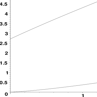
Figure 1: Plots of $-\ell/W_{-1}\left(-\frac{\ell}{e\,(1+\ell)}\right)$ and $-\ell/W_{0}\left(-\frac{\ell}{e\,(1+\ell)}\right)$.

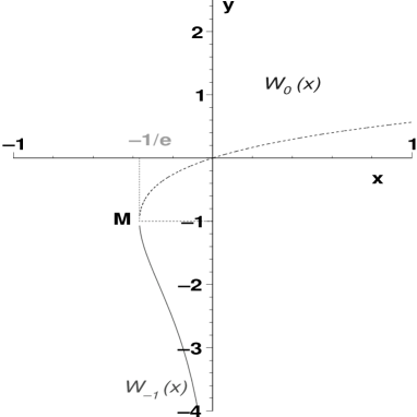
Figure 2: The branches $W_{0}$ (dashed line) and $W_{-1}$ (solid line) of the Lambert W function.

References

- [1] Akyildiz, I. F., Su, W., Sankarasubramaniam, Y. and Cayirci, E. Wireless sensor networks: a survey. Computer Networks 38: 393–422, 2002.
- [2] Alon, N., and Spencer, J. The Probabilistic Method. Wiley, New-York, 1992.
- [3] Bar-Yehuda, R., Goldreich, O. and Itai, A. Efficient Emulation of Single-Hop Radio Network with Collision Detection on Multi-Hop Radio Network with no Collision Detection. Distributed Computing, 5: 67–71, 1991.
- [4] Bar-Yehuda, R., Goldreich, O. and Itai, A. On the Time-Complexity of Broadcast in Multi-Hop Radio Networks: An Exponential Gap between Determinism and Randomization. Journal of Comp. and Sys. Sciences, 45: 104–126, 1992.
- [5] Basagni, S. and Chlamtac, I. A Mobility-Transparent Deterministic Broadcast Mechanism for Ad Hoc Networks. IEEE/ACM Trans. on Networking 7:799–807, 1999.
- [6] Battiti, R., Bertossi, A. A. and Bonuccelli, M. A. Assigning Codes in Wireless Networks: Bounds and Scaling Properties. Wireless Networks 5:195–209, 1999.
- [7] Berkeley Wireless Research Center: http://bwrc.eecs.berkeley.edu.
- [8] Bettstetter, C. On the Minimum Node Degree and Connectivity of a Wireless Multihop Network. Proc. of ACM Mobihoc’02, pp 80–91, 2002.
- [9] Bollobás, B. Random Graphs. Academic Press, London, 1985.
- [10] Cayley, A. A Theorem on Trees. Quart. J. Math. Oxford Ser., 23: 376–378, 1889.
- [11] Center for Embedded Networked Sensing: http://cens.ucla.edu/
- [12] Chatzigiannakis, L., Nikoletseas, S. and Spirakis, P. Efficient and Robust Protocols for Local Detection and Propagation in Smart Dust Protocols. To appear in ACM/Kluwer Mobile Networks and Applications, 2004.
- [13] Cheng, Y.-C. and Robertazzi T. G. Critical connectivity phenomena in multihop radio models. IEEE Trans. on Communications, 36: 770–777, 1989.
- [14] Corless, R. M., Gonnet G. H., Hare D. E. G., Jeffrey D. J. and Knuth D. E. On the Lambert W Function. Advances in Computational Mathematics, 5: 329–359, 1996.
- [15] De Bruijn, N. G. Asymptotic Methods in Analysis. Dover, New-York, 1981.
- [16] Dousse, O., Thiran, P. and Hasler, M. Connectivity in Ad Hoc and Hybrid Network. Proceedings of INFOCOM, 2002.
- [17] Erdős, P. and Rényi A. On the evolution of random graphs. Publ. Math. Inst. Hung. Acad. Sci., 5:17–61, 1960.
- [18] Estrin, D., Govindan, R., Heidemann, J. and Kumar S. Next century challenges: Scalable coordination in sensor networks. Proceedings of IEEE/ACM International Conference on Mobile Computing and Networking, pp 263–270, 1999.
- [19] Finocchi, I., Panconesi, A. and Silvestri, R. Experimental Analysis of Simple, Distributed Vertex Coloring Algorithms. Proceedings of ACM-SIAM Symposium on Discrete Algorithms, pp 606–615, 2002.
- [20] Friedgut, E. and Kalai, G. Every Monotone Graph Property Has a Sharp Threshold. Proc. Amer. Math. Soc., vol. 124, pp. 2993–3002, 1996.
- [21] Gautschi, W. The Incomplete Gamma Functions Since Tricomi. In Tricomi’s Ideas and Contemporary Applied Mathematics. Atti dei Convegni Lincei, Accademia Nazionale dei Lincei, Roma, 147:203–237, 1998.
- [22] Gilbert, E. N. Random Plane Networks. Journal of the Society for Industrial and Applied Math, 9: 533–543, 1961.
- [23] Goel, A., Sanatan, R. and Krishnamachari, B. Sharp thresholds for monotone properties in random geometric graphs. To appear in the ACM Symposium on Theory of Computing, 2004.
- [24] Gupta, P. and Kumar P. R. Critical power for asymptotic connectivity in wireless networks. Stochastic Analysis, Control, Optimization and Applications: a volume in honor of W. H. Fleming, W. M. McEneaney, G. Yin and Q. Zhang, Birkhäuser, Boston, 1998.
- [25] Gupta, P. and Kumar P. R. Internet in the Sky: The Capacity of Three Dimensional Wireless Networks. Communications in Information and Systems, 1:33–49, 2001.
- [26] Hall, P. Introduction to the Theory of Coverage Processes. Birkhäuser, Boston, 1988.
- [27] Hu, L. Distributed code assignments for CDMA Packet Radio Network. IEEE/ACM Transactions on Networking Vol 1: 668–677, 1993.
- [28] Hong, X., Gerla, M. and Wang H. Load-Balance, Energy-Aware Communication for Mars Sensor Network. in Proceedings of IEEE Aerospace Conference, 2002.
- [29] Janson, S., Knuth, D. E., Luczak, T. and Pittel B. The birth of the giant component. Random Structures & Algorithms, 4:233–358, 1993.
- [30] Janson, S., Luczak, T. and Rucinski A. Random Graphs. John Wiley, New York, 2000.
- [31] Jung, E-S and Vaidya N. A Power Control MAC Protocol for Ad Hoc Networks. Proc. of ACM Mobicom’02, pp. 36–47, 2002.
- [32] Krishnamachari, B., Wicker S. B. and Bejar R. Phase Transition Phenomena in Wireless Ad-Hoc Networks. Proc. of IEEE GlobeCom’01, 2001.
- [33] Krishnamachari, B., Bejar R. and Wicker S. B. Distributed Problem Solving and the Boundaries of Self-Configuration in Multi-hop Wireless Networks. In Proc. of 35th Hawaii Int. Conf. on System Sciences, 2001.
- [34] Krishnamachari, B., Wicker S. B., Bejar R. and Pearlman M. Critical Density Thresholds in Distributed Wireless Networks. Book chapter in Communications, Information and Network Security, eds. H. Bhargava, H.V. Poor, V. Tarokh, and S. Yoon, Kluwer Publishers, 2002.
- [35] Li, D., Wong, K. and Sayeed A. Detection, Classification and Tracking of Targets in Distributed Sensor Networks. IEEE Signal Processing Magazine, Vol. 19 Issue 2, March 2002.
- [36] Malpani, N., Welch J. L. and Vaidya, N. Leader election algorithms for mobile ad hoc networks. in Proceedings of the 4th international workshop on Discrete algorithms and methods for mobile computing and communications, pp 96–103, 2000.
- [37] Molloy, M. and Reed, B. Graph Colouring and the Probabilistic Method. Springer, Berlin, 2002.
- [38] McDiarmid, C. Random Channel Assignment in the Plane. Random Structures & Algorithms, 22: 187–212, 2003.
- [39] Meester, R. and Roy, R. Continuum Percolation. Cambridge University Press, Cambridge, 1996.
- [40] Meguerdichian, S., Koushanfar, F., Potkonjak, M. and Srivastava M. B. Coverage Problems in Wireless Ad-hoc Sensor Networks. Proc. of IEEE Infocom’01, pp. 1380–1387, 2001.
- [41] Meguerdichian, S., Koushanfar, F., Qu, G. and Potkonjak, M. Exposure in Wireless Ad-Hoc Sensor Networks. Proc. of ACM Mobicom’01, pp. 139–150, 2001.
- [42] Miles, R. E. On the Homogeneous Planar Poisson Point Process. Math. Biosciences, 6: 85–127, 1970.
- [43] Miles, R. E. Asymptotic coverage and concentration probabilities for Poisson spheres. Annals of Mathematical Stat., 40: 1160, 1969.
- [44] Nasa/JPL Sensor Webs Project: http://sensorwebs.jpl.nasa.gov/.
- [45] Penrose, M. D. The longest edge of the random minimal spanning tree. Annals of Applied Probability, 7: 340–361, 1997.
- [46] Penrose, M. D. On -connectivity for a geometric random graph. Random Structures & Algorithms, 15: 145–164, 1999.
- [47] Penrose, M. D. Random Geometric Graphs. Oxford Studies in Probability, 2003.
- [48] Perkins, C. E. Ad Hoc Networking. Addison-Wesley, 2001.
- [49] Philips, T. K., Panwar, S. S. and Tantawi, A. N. Connectivity properties of a packet radio network model. IEEE Trans. on Inf. Theory, 35: 1044–1047, 1989.
- [50] Piret, P. On the Connectivity of Radio Networks. IEEE Trans. on Inf. Theory, 37: 1490–1492, 1991.
- [51] Proakis, J. G., Sozer, E. M., Rice, J. A. and Stojanovic, M. Shallow Water Acoustic Networks. IEEE Communications Magazine, 39: 114–119, 2001.
- [52] Ravelomanana, V. Asymptotic Critical Ranges for Coverage Properties in Wireless Sensor Networks. Technical Report – Université de Paris XIII (submitted).
- [53] Santalo, L. Integral Geometry and Geometric Probability. Cambridge University Press, 2003.
- [54] Santi, P. and Blough D. M. The Critical Transmitting Range for Connectivity in Sparse Wireless Ad Hoc Networks. IEEE Trans. Mob. Comp., 2: 1–15, 2003.
- [55] Shakkottai, S., Srikant, R. and Shroff N., Unreliable Sensor Grids: Coverage, Connectivity and Diameter. To appear in Ad Hoc Networks (2004). Previous version was published in Proceedings of IEEE Infocom 2003.
- [56] Temme, N. Uniform asymptotic expansions of the incomplete gamma functions and the incomplete beta functions. Math. Comput., 29: 1109–1114, 1975.
- [57] Temme, N. The asymptotic expansion of the incomplete gamma function. SIAM J. Math. Anal., 10: 757–766, 1979.
- [58] Wireless Integrated Sensor Networks: http://www.janet.ucla.edu/WINS.
- [59] Xu, Y., Heidemann, J. S. and Estrin, D. Geography-informed energy conservation for Ad Hoc routing. Proc. of ACM Mobicom’01, pp. 70–84, 2001.
- [60] Xue, F. and Kumar, P. R. The number of neighbors needed for connectivity of wireless networks. Wireless Networks, 10: 169–181, 2004.