Basic properties for sand automata

Abstract

We prove several results about the relations between injectivity and surjectivity for sand automata. Moreover, we begin the exploration of the dynamical behavior of sand automata proving that the property of nilpotency is undecidable. We believe that the proof technique used for this last result might reveal useful for many other results in this context.

Keywords: sand automata, reversibility, undecidability

1 Introduction

Self-organized criticality (SOC) is a notion which tries to explain the peculiar behavior of many natural and physical phenomena. These systems evolve, according to some law, to a “critical state”. Any perturbation, no matter how small, of the critical state generate a deep spontaneous re-organization of the system. Thereafter, the system evolves to another critical state and so on.

Example of SOC systems are: sandpiles, snow avalanches, star clusters in the outer space, earthquakes, forest fires, load balance in operating systems [1, 3, 2, 4, 14].

Sandpiles models are a paradigmatic formal model for SOC systems [10, 11]. In [5], the authors introduced sand automata as a generalization of sandpiles models and transposed them in the setting of discrete dynamical systems. A key-point of [5] was to introduce a suitable topology and study the dynamical behavior of sand automata w.r.t. this new topology. This resulted in a fundamental representation theorem similar to the well-known Hedlund’s theorem for cellular automata [5, 13].

This paper continues the study of sand automata starting from basic set properties like injectivity and surjectivity. The decidability of those two last properties is still an open question. In order to simplify the decision problem we study the relations between basic set properties. We prove that many relations between set properties that are true in cellular automata are no more true in the context of sand automata. This allows to conclude that sand automata are a completely new model and not a peculiar “sub-model” of cellular generalized automata as it might seem at a first glance.

In particular, we show that injective sand automata are not necessarily reversible but they might have a right inverse automaton which is not a left inverse. This is a completely new situation w.r.t. cellular automata which we think is worthwhile future studies.

Understanding the dynamical behavior of sand automata is in general very difficult. Hence we started from very “simple” behavior: nilpotency. Roughly speaking, a sand automaton is nilpotent if from any starting point it reaches a constant configuration after a finite number of iterations. We have proved (Theorem 18) that the problem of establishing if a given automaton is nilpotent is undecidable (when considering spatial periodic or finite configurations).

We believe that the proof technique developed for Theorem 18 might be used for proving many other similar results.

The paper is structured as follows. The next section introduces the topology on sandpiles and related known results. Section 3 recalls the definition of sand automata and their representation theorem. Very interesting and useful examples of sand automata are presented in Section 4. The main results are in Sections 5 and 6. In Section 7 we draw our conclusions.

Remark that, due to lack of space, some results have no proof. Their proofs can be found in the appendix.

2 The topology on sandpiles

A configuration represents a set of sand grains, organized in piles and distributed all over a $d$-dimensional grid. With every point of the grid $\mathbb{Z}^{d}$ is associated with the number of grains i.e. an element of $\widetilde{\mathbb{Z}}=\mathbb{Z}\cup\{-\infty,+\infty\}$. The value $-\infty$ represents a sink and $+\infty$ a source of sand grains. Hence a configuration is an element of $\widetilde{\mathbb{Z}}^{\mathbb{Z}^{d}}$. We will denote by $c_{i_{1},\ldots,i_{d}}$ or $c_{i}$ the number of grains in the column of $c$ indexed by the vector $i=(i_{1},\ldots,i_{d})$. Finally, for $i\in\widetilde{\mathbb{Z}}$, $\mathfrak{E}_{i}$ is the set of configurations with the value $i$ at position $(0,\ldots,0)$. Denote $\mathfrak{C}$ the set of all configurations.

A configuration $c$ is finite if $\exists k\in\mathbb{N}$ such that for any vector $i\in\mathbb{Z}^{d}$, $|i|\geq k$, $c_{i}=0$ (remark that we denote by $|\cdot|$ the infinite norm). The set of finite configurations will be noted $\mathfrak{C}$. A configuration $c$ is periodic if there is a vector $p\in\mathbb{Z}^{d}$ such that for any vector $i\in\mathbb{Z}^{d}$ and any integer $t\in\mathbb{Z}$, $c_{i}=c_{i+tp}$; $\mathfrak{C}$ denotes the set of periodic configurations.

In the remainder of the section, definitions are only given for dimension $1$. The generalization to higher dimensions is straightforward.

In [5], the authors equipped $\mathfrak{C}$ with a metric topology defined in two steps. First, one fixes a reference point (for example the column of index $0$); then the metric is designed in such a way that two configurations are at small distance if the have “the same” number of grains in a (finite) neighborhood of the reference point. Of course, one should make more precise the meaning of the sentence “have the same grains content”. The differences in the number of grains is quantified by a measuring device of size $l\in\mathbb{N}$ and reference height $m\in\mathbb{Z}$

$$\beta_{l}^{m}(n)=\left\{\begin{array}[]{c@{\hspace{5mm}}l}+\infty\hfil\hskip 14.22636pt&\textrm{if $n>m+l$}\enspace,\\ -\infty\hfil\hskip 14.22636pt&\textrm{if $n<m-l$}\enspace,\\ n-m\hfil\hskip 14.22636pt&\textrm{otherwise}.\end{array}\right.$$

If the difference (in the number grains) between two columns is too high (resp. too low), then it is declared to be $+\infty$ (resp. $-\infty$).

For any configuration $c\in\widetilde{\mathbb{Z}}^{\mathbb{Z}}$, $l\in\mathbb{N}$, $l\neq 0$ and $i\in\mathbb{Z}$, define the following sequence of differences:

$$d_{l}^{i}(c)=\left\{\begin{array}[]{l@{\hspace{5mm}}l}(\beta_{l}^{c_{i}}(c_{i-l}),\ldots,\beta_{l}^{c_{i}}(c_{i-1}),\beta_{l}^{c_{i}}(c_{i+1}),\ldots,\beta_{l}^{c_{i}}(c_{i+l}))\hfil\hskip 14.22636pt&\textrm{if $|c_{i}|\neq\infty$}\enspace,\\[4.30554pt] (\beta_{l}^{0}(c_{i-l}),\ldots,\beta_{l}^{0}(c_{i-1}),\beta_{l}^{0}(c_{i+1}),\ldots,\beta_{l}^{0}(c_{i+l}))\hfil\hskip 14.22636pt&\textrm{if $c_{i}=\pm\infty$}\enspace.\\ \end{array}\right.$$

For $l=0$, define $d_{0}^{i}(c)=(c_{i})$. Finally, the distance between two configurations $x$ and $y$ is defined as follows: $d(x,y)=2^{-l}$, where $l$ is the smallest integer such that $d_{l}^{0}(x)\neq d_{l}^{0}(y)$.

From now on, $\mathfrak{C}$ is equipped with the metric topology induced by $d$. The following propositions prove that the structure of the topology on $\mathfrak{C}$ is rich enough to justify the study of dynamical systems on it.

Proposition 1 ([5])

The space $\mathfrak{C}$ is perfect (i.e. it has no isolated point) and locally compact (i.e. for any point $x$ there is a neighborhood of $x$ whose closure is compact).

Proposition 2 ([5])

The space $\mathfrak{C}$ is totally disconnected (i.e. for any points $x,y$ there are two open sets $U$ and $V$ such as $x\in U$, $y\in V$, $U\cap V=\emptyset$ and $U\cup V=\mathfrak{C}$).

Proposition 3 ([5])

For any $i\in\widetilde{\mathbb{Z}}$, the set $\mathfrak{E}_{i}$ is compact.

The following result completes the characterization of the topological structure of $\mathfrak{C}$.

Proposition 4

The space $\mathfrak{C}$ is complete.

3 Sand automata

A sand automaton (SA) is a deterministic automaton acting on configurations. It essentially consists in a local rule which is applied in parallel to each column of the current configuration. The local rules quantifies the grain content of a neighborhood of the current column to decide the amount of grains that this columns gains or loses.

In the sequel, we give the formal definition of sand automaton in dimension $1$. Its generalization to higher dimensions is straightforward.

Formally, a sand automaton is a structure $\mathcal{A}\equiv\langle r,\lambda\rangle$ where $\lambda:\widetilde{[\![-r,r]\!]}^{2r}\rightarrow[\![-r,r]\!]$ is the local rule and $r$ is the “size” (sometimes also called the radius) of the measuring device. The global function $f_{\mathcal{A}}:\mathfrak{C}\rightarrow\mathfrak{C}$ of $\mathcal{A}$ is defined as follows

$$\forall c\in\mathfrak{C}\forall i\in\mathbb{Z},\quad f_{\mathcal{A}}(c)_{i}=\left\{\begin{array}[]{l@{\hspace{5mm}}l}c_{i}\hfil\hskip 14.22636pt&\textrm{if $c_{i}=\pm\infty$}\enspace,\\ c_{i}+\lambda(d_{r}^{i}(c))\hfil\hskip 14.22636pt&\textrm{otherwise}.\end{array}\right.$$

In [5], the authors show that sand automata can easily simulate all sandpile models known in literature and even cellular automata. They also obtained the following fundamental representation result; but let us first introduce a few more useful definitions.

We need two special functions: the shift map $\sigma:\mathfrak{C}\rightarrow\mathfrak{C}$ defined by $\forall c\in\mathfrak{C},\forall i\in\mathbb{Z},\quad\sigma(c)_{i}=c_{i+1}$ ; and the raising map $\rho:\mathfrak{C}\rightarrow\mathfrak{C}$ defined by $\forall c\in\mathfrak{C}\forall i\in\mathbb{Z},\quad\rho(c)_{i}=c_{i}+1$. A function $f:\widetilde{[\![-r,r]\!]}^{2r}\rightarrow[\![-r,r]\!]$ is shift invariant (resp. vertical invariant) if $f\circ\sigma=\sigma\circ f$ (resp. $f\circ\rho=\rho\circ f$). A function $f:\widetilde{[\![-r,r]\!]}^{2r}\rightarrow[\![-r,r]\!]$ is infiniteness conserving if

$$\forall c\in\mathfrak{C}\forall i\in\mathbb{Z},\quad\left\{\begin{array}[]{lcl}f(c)_{i}=+\infty&\Leftrightarrow&c_{i}=+\infty\\ \qquad\textrm{and}\\ f(c)_{i}=-\infty&\Leftrightarrow&c_{i}=-\infty\enspace.\end{array}\right.$$

Theorem 5 ([5])

A function $f:\mathfrak{C}\rightarrow\mathfrak{C}$ is the global function of a sand automaton if and only if $f$ is continuous, shift-invariant, vertical-invariant and infiniteness conserving.

By an abuse of terminology, we will often confuse a sand automaton $\mathcal{A}\equiv\langle r,\lambda\rangle$ with its global function $f_{\mathcal{A}}$. For example, we will say that $\mathcal{A}$ is surjective (resp. injective) if $f_{\mathcal{A}}$ is surjective (resp. injective). For $\mathfrak{U}\subseteq\mathfrak{C}$, $f_{\mathcal{A}}$ is said to be $\mathfrak{U}$-surjective (resp. injective) if the restriction of $f$ to $\mathfrak{U}$ is surjective (resp. injective).

4 Examples

In this section we introduce a series of worked examples with a twofold purpose: illustrate basic behavior of sand automata and constitute a set of counter-examples for later use. Some examples might seem a bit technical but the underlaying ideas are very useful in the sequel.

Example 1

The automaton $\mathcal{S}$.
This automaton is to the simulation of SPM in dimension $1$: $\mathcal{S}=\langle 1,\lambda_{\mathcal{S}}\rangle$, where

$$\forall x,y\in\widetilde{[\![-1,1]\!]},\quad\lambda_{\mathcal{S}}(x,y)=\left\{\begin{array}[]{r@{\hspace{5mm}}l}+1\hskip 14.22636pt&\textrm{if $x=+\infty$ and $y\neq-\infty$}\enspace,\\ -1\hskip 14.22636pt&\textrm{if $x\neq+\infty$ and $y=-\infty$}\enspace,\\ 0\hskip 14.22636pt&\textrm{otherwise.}\end{array}\right.$$

Remark the basic grain movement of $\mathcal{S}$: a grain falls to the column on its right when the height difference is bigger than $2$.

Example 2

The automaton $\mathcal{S}^{r}$.
This automaton is defined similarly to $\mathcal{S}$, but grains climb the cliffs instead of falling down.Let $\mathcal{S}^{r}=\langle 1,\lambda_{\mathcal{S}^{r}}\rangle$ where

$$\forall x,y\in\widetilde{[\![-1,1]\!]},\quad\lambda_{\mathcal{S}^{r}}(x,y)=\left\{\begin{array}[]{r@{\hspace{5mm}}l}-1\hskip 14.22636pt&\textrm{if $x=+\infty$ and $y\neq-\infty$}\enspace,\\ +1\hskip 14.22636pt&\textrm{if $x\neq+\infty$ and $y=-\infty$}\enspace,\\ 0\hskip 14.22636pt&\textrm{otherwise.}\end{array}\right.$$

Proposition 6

The SA $\mathcal{S}$ is $\mathfrak{U}$-surjective for $\mathfrak{U}=\mathfrak{C},\mathfrak{F},\mathfrak{P}$. The SA $\mathcal{S}^{r}$ is $\mathfrak{U}$-injective for $\mathfrak{U}=\mathfrak{C},\mathfrak{F},\mathfrak{P}$.

Proof. It is not difficult to see that $\mathcal{S}\circ\mathcal{S}^{r}=id$, but $\mathcal{S}^{r}\circ\mathcal{S}\neq id$. The first equation implies that $\mathcal{S}$ is surjective and $\mathcal{S}^{r}$ is injective. Moreover, since the pre-image by $\mathcal{S}$ of a configuration is computed by $\mathcal{S}^{r}$, another SA, the pre-image of a finite configuration is finite, and periodic if the initial configuration was periodic. Hence we have the first part of the thesis. The second part is a consequence of the injectivity of $\mathcal{S}^{r}$. ❏

Proposition 7

The SA $\mathcal{S}$ is not $\mathfrak{U}$-injective for $\mathfrak{U}=\mathfrak{C},\mathfrak{F},\mathfrak{P}$.

Proposition 8

The SA $\mathcal{S}^{r}$ is not $\mathfrak{U}$-surjective for $\mathfrak{U}=\mathfrak{C},\mathfrak{F},\mathfrak{P}$.

Example 3

The automaton $\mathcal{L}$.
Consider an automaton $\mathcal{L}=\langle 1,\lambda_{\mathcal{L}}\rangle$ where

$$\forall x,y\in\widetilde{[\![-1,1]\!]},\quad\lambda_{\mathcal{L}}(x,y)=\left\{\begin{array}[]{r@{\hspace{5mm}}l}-1\hskip 14.22636pt&\textrm{if $x<0$}\enspace,\\ +1\hskip 14.22636pt&\textrm{if $x>0$}\enspace,\\ 0\hskip 14.22636pt&\textrm{otherwise.}\end{array}\right.$$

Remark the basic behavior of $\mathcal{L}$: each column tries to reach the same height of its left neighbor.

Proposition 9

The SA $\mathcal{L}$ is not $\mathfrak{F}$-surjective.

Proposition 10

The SA $\mathcal{L}$ is both $\mathfrak{C}$-surjective and $\mathfrak{P}$-surjective.

Proof. Choose an arbitrary configuration $c$, we are going to build one of its pre-image $c^{\prime}$. There is a unique sequence of strictly increasing indices $(i_{n})_{n\in N}$, $N\subset\mathbb{Z}$, such that $\forall i_{n}\leq i<i_{n+1},\quad c_{i}=c_{i_{n}}$ and $c_{i_{n}}\neq c_{i_{n}-1}$ (every $i_{n}$ corresponds to a variation in $c$). The idea is to work on these intervals, amplifying the difference at the border so that an application of the rule corrects it. Formally, for every $n\in N$, suppose that $c_{i_{n}-1}<c_{i_{n}}$ (if it is not the case then the symmetrical operations will have to be performed). For every $i_{n}\leq i<i_{n+1}$, let $c^{\prime}_{i}=c_{i}+1$ if $i-i_{n}$ is even, $c^{\prime}_{i}=c_{i}-1$ if $i-i_{n}$ is odd. There are two little subtleties if $N$ is not bi-infinite. If $n_{0}=\inf N$ exists, then let $c^{\prime}_{i}=c_{i}$ for all $i<n_{0}$. One could prefer to make it more consistent with the rest and choose $c^{\prime}_{i}=c_{i}\pm 1$ according to the parity of $i$, it does not matter much. Second, if $n_{1}=\sup N$ exists, then the $\pm$ operation has to be performed forever on the right. Note that it is why a finite configuration may not have a finite pre-image.

It is not difficult to see that $f_{\mathcal{L}}(c^{\prime})=c$. For every $i\in\mathbb{Z}$, first suppose that there is a $n\in N$ such that $i=i_{n}$. We have $f_{\mathcal{L}}(c^{\prime})_{i}=c^{\prime}_{i}+\lambda_{\mathcal{L}}(d^{i}_{1}(c^{\prime}))$. Supposing that $c_{i-1}<c_{i}$ (again, if it is the opposite then the operations are symmetrical), we have $c^{\prime}_{i}=c_{i}+1>c_{i-1}+1$, hence $c^{\prime}_{i}>c^{\prime}_{i-1}$ since $|c_{i-1}-c^{\prime}_{i-1}|\leq 1$ . So $\lambda_{\mathcal{L}}(d^{i}_{1}(c^{\prime}))=-1$, and $f_{\mathcal{L}}(c^{\prime})_{i}=c_{i}+1-1=c_{i}$. Otherwise if $i\neq i_{n}$ for all $n\in N$, then by construction we have either:

• $c^{\prime}_{i}=c_{i}+1$ and $c^{\prime}_{i-1}=c_{i-1}-1=c_{i}-1$, because $c$ is constant between the $i_{n}$’s. Hence $c^{\prime}_{i-1}=c^{\prime}_{i}-2$, and then $f_{\mathcal{L}}(c^{\prime})_{i}=c_{i}+1-1=c_{i}$ ;

• or $c^{\prime}_{i}=c_{i}-1$ and $c^{\prime}_{i-1}=c_{i-1}+1$, the same method gives the result.

Therefore $\mathcal{L}$ is surjective. Finally, as the operations we perform on the configuration are deterministic, a periodic configuration would have a periodic pre-image (same transformation of the period everywhere). Hence $\mathcal{L}$ is also surjective over periodic configurations. ❏

The next example is a bit less intuitive since it uses a special neighborhood: the two nearest left neighbors.

Example 4

The automaton $\mathcal{X}$.
Consider the sand automaton $\mathcal{X}=\langle 2,\lambda_{\mathcal{X}}\rangle$ where

$$\begin{array}[]{l@{\hspace{5mm}}l}\forall x,y,z\in\widetilde{[\![-2,2]\!]},\hfil\hskip 14.22636pt&\lambda_{\mathcal{X}}(+\infty,x,y,z)=-1\enspace,\\ \hfil\hskip 14.22636pt&\lambda_{\mathcal{X}}(2,x,y,z)=-1\enspace,\\ \hfil\hskip 14.22636pt&\lambda_{\mathcal{X}}(1,-1,x,y)=-1\enspace,\\ \hfil\hskip 14.22636pt&\lambda_{\mathcal{X}}(1,-2,x,y)=-1\enspace,\\ \hfil\hskip 14.22636pt&\lambda_{\mathcal{X}}(1,-\infty,x,y)=-1\enspace,\\ \hfil\hskip 14.22636pt&\lambda_{\mathcal{X}}(0,-2,x,y)=-1\enspace,\\ \hfil\hskip 14.22636pt&\lambda_{\mathcal{X}}(0,-\infty,x,y)=-1\enspace,\end{array}$$

and any other value gives $0$. The behavior of this automaton on two specific sequences is shown in Figure 1. The evolutions of $\mathcal{X}$ on more general configurations seem quite hard to describe. Anyway, in the sequel we will need to study its evolutions only on special (simple) configurations.

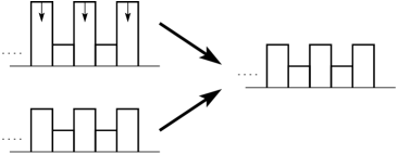
Figure 1: examples of evolution of $\mathcal{X}$ on two different configurations.

Proposition 11

The SA $\mathcal{X}$ is $\mathfrak{F}$-injective but not $\mathfrak{C}$- or $\mathfrak{P}$-injective.

Example 5

The automaton $\mathcal{Y}$.
Consider the following SA $\mathcal{Y}=\langle 2,\lambda_{\mathcal{Y}}\rangle$, where

$$\begin{array}[]{l@{\hspace{5mm}}l}\forall x,y,z\in\widetilde{[\![-2,2]\!]},\hfil\hskip 14.22636pt&\lambda_{\mathcal{Y}}(+\infty,x,y,z)=-1\enspace,\\ \hfil\hskip 14.22636pt&\lambda_{\mathcal{Y}}(2,x,y,z)=-1\enspace,\\ \hfil\hskip 14.22636pt&\lambda_{\mathcal{Y}}(1,x,y,z)=-1\enspace,\\ \hfil\hskip 14.22636pt&\lambda_{\mathcal{Y}}(0,x,y,z)=-1\enspace,\\ \hfil\hskip 14.22636pt&\lambda_{\mathcal{Y}}(-1,-\infty,x,y)=-1\enspace,\\ \end{array}$$

and everything else returns $0$. Figure 2 shows two meaningful behaviors of the automaton that will be used later.

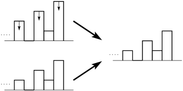
Figure 2: examples of the action of $\mathcal{Y}$.

Proposition 12

The SA $\mathcal{Y}$ is $\mathfrak{F}$- and $\mathfrak{P}$-injective, but not injective.

Proof. Consider the two configurations $c$ and $c^{\prime}$ defined as follows

$$\forall i\in\mathbb{Z},\qquad\left\{\begin{array}[]{l}c_{2i}=i\\ c_{2i+1}=i+2\enspace,\end{array}\right.\quad\left\{\begin{array}[]{l}c^{\prime}_{2i}=i\\ c^{\prime}_{2i+1}=i+3\enspace.\end{array}\right.$$

It is not difficult to see that $f_{\mathcal{Y}}(c)=f_{\mathcal{Y}}(c^{\prime})=c$ (see also Figure 2). Hence $\mathcal{Y}$ is not injective. In order to show that $\mathcal{Y}$ is injective over finite and periodic configurations, we will need an intermediate result: if $c$, $c^{\prime}$ are two distinct configurations such that $f_{\mathcal{Y}}(c)=f_{\mathcal{Y}}(c^{\prime})$, then there are infinitely many differences, of infinitely many different values. Practically, we will show that if $c_{i}>c^{\prime}_{i}$ then $c_{i-2}>c^{\prime}_{i-2}$ and $c_{i-2}<c_{i}$.

Assume $c_{i}>c^{\prime}_{i}$ for some $i$, and let $f(c)=f(c^{\prime})$. Then, without loss of generality, one can choose $c_{i}=c^{\prime}_{i}+1$ (the difference can not be greater than one, because $\lambda_{\mathcal{Y}}$ only returns $-1$ or $0$). Therefore, a rule which returns $0$ is applied to $c^{\prime}$ at position $i$, which means that $c^{\prime}_{i-2}\leq c^{\prime}_{i}-1$ (since $\lambda_{\mathcal{Y}}(x,-,-,-)$ returns $0$ only if $x\leq-1$). For the same reason, one of the five rules which returns $-1$ is applied to $c$ at position $i$, hence $c_{i-2}\geq c_{i}-1$. So $c_{i-2}\geq c_{i}-1=c^{\prime}_{i}\geq c^{\prime}_{i-2}+1>c^{\prime}_{i-2}$. The first consequence of this inequality is that if there is a difference somewhere, there are infinitely many differences, hence $\mathcal{Y}$ is $\mathfrak{F}$-injective. Indeed two finite configurations cannot have infinitely many differences, so two different finite configurations have a different image.

Moreover, $c_{i-2}=c^{\prime}_{i-2}+1$ to ensure $f_{\mathcal{Y}}(c)=f_{\mathcal{Y}}(c^{\prime})$. So the inequalities above are in reality equalities, in particular $c_{i-2}=c_{i}-1$. Therefore it holds $\cdots<c_{i-4}<c_{i-2}<c_{i}$, which proves that two different periodic configurations also have different images (a periodic configuration contains a finite number of different columns, which is contradicted by the above inequality). As a consequence, $\mathcal{Y}$ is $\mathfrak{P}$-injective. ❏

5 Basic set properties

This section concerns the relations between surjectivity and injectivity, w.r.t. all, finite and periodic configurations, in the same way it was done in [7] for cellular automata. In particular the relation between $\mathfrak{F}$-injectivity and surjectivity was interesting, as for cellular automata it can be used to prove undecidability of surjectivity [6]. Unfortunately, there is not relation between those two properties in the context of SA (see Propositions 6, 7, 8). In this section we try to analyze these relation deeper hoping this might help for the proof of the decidability result about surjectivity or injectivity.

Proposition 13

$\mathfrak{F}$-surjectivity implies surjectivity.

Proof. For any configuration $c$, let $c^{0}_{n}$ be such that $\forall i\in\mathbb{Z},\;(c^{0}_{n})_{i}=c_{i}$ if $-n\leq i\leq n$ and $(c^{0}_{n})_{i}=0$ otherwise. Consider a sand automaton $f$ that is $\mathfrak{F}$-surjective and choose an arbitrary configuration $c\in\mathfrak{C}$. For any $n\in\mathbb{N}$, let $c_{n}=f^{-1}(c^{0}_{n})$. The pre-images $c_{n}$ are contained in some set $E_{i}$ for $i\in I$, with $\left|I\right|<\infty$. Since $\cup_{i\in I}E_{i}$ is compact and $(c_{n})_{n\in\mathbb{N}}\subset\cup_{i\in I}E_{i}$, $(c_{n})_{n\in\mathbb{N}}$ contains a converging sub-sequence $(c_{n_{i}})_{i\in\mathbb{N}}$. Let $c^{*}=\lim_{i\to\infty}c_{n_{i}}$. By contradiction, assume that $f(c^{*})\neq c$. Then there exists $j\in\mathbb{Z}$ such that $f(c^{*})_{j}\neq c_{j}$ but $f(c_{n_{i}})_{j}=c_{j}$ for $n_{i}$ big enough. ❏

Remark that the result of Proposition 13 is true in any dimension but the opposite implication is false (even in dimension $1$), since $\mathcal{L}$ which is surjective but not $\mathfrak{F}$-surjective (see Propositions 9 and 10).

Proposition 14

$\mathfrak{P}$-surjectivity implies $\mathfrak{C}$-surjectivity.

Proposition 15

In dimension $1$, $\mathfrak{C}$-surjectivity implies $\mathfrak{P}$-surjectivity.

Proof. Let $\mathcal{A}$ be a surjective sand automaton in dimension 1, and $c^{0}$ a periodic configuration of period $p\in\mathbb{Z}$. Let $c$ be a pre-image of $c^{0}$ by $\mathcal{A}$. We will build a periodic configuration from $c$, whose image will be $c^{0}$. Let $X=\{(c_{k-r},\ldots,c_{k+r-1})\>|\>\exists\alpha\in\mathbb{Z},k=\alpha p\}$. Since for every $i\in\mathbb{Z}$, $|c_{i}-c^{0}_{i}|\leq r$ (as $\lambda$ returns an element of $[\![-r,r]\!]$), and because $c^{0}$ is $p$-periodic, there are at most $2r\cdot(2r+1)$ elements in $X$. Let $k_{1}=\alpha_{1}p$ and $k_{2}=\alpha_{2}p$, $k_{1}<k_{2}$ such that $(c_{k_{1}-r},\ldots,c_{k_{1}+r-1})=(c_{k_{2}-r},\ldots,c_{k_{2}+r-1})$. Let the $(k_{2}-k_{1})$-periodic configuration $c^{\prime}$ where the period is defined by (see Figure 3 for the construction) $c^{\prime}_{k_{1}+i}=c_{k_{1}+i}$ for all $0\leq i<k_{2}-k_{1}$ .

Figure 3: Construction of $c^{\prime}$ using $c$

It is easy to see that $f(c^{\prime})=c^{0}$, because for every configuration of the period of $c^{\prime}$, the automaton sees the same neighborhood as for $c$ (due to the construction of $c^{\prime}$), so it acts in the same correct way. And as $k_{2}-k_{1}$ is a multiple of $p$, each period of $c^{\prime}$ coincides with a period of $c^{0}$, so the image of $c^{\prime}$ is equal to $c$ everywhere: $\mathcal{A}$ is $\mathfrak{P}$-surjective. ❏

In dimensions greater than $1$, the above problem is currently open, we have no direct proof nor counter-example. The problem is due to the fact that in dimension $2$ and above, the size of the perimeter of a ball (the $2r$ sequence we used in X for the proof in dimension $1$) is linked to the size of the ball. Therefore we can not say that there is a finite number of perimeters, and then stick them together to build the periodic configuration.

Corollary 16

In dimension $1$, $\mathfrak{F}$-surjectivity implies $\mathfrak{P}$-surjectivity.

The question if the above corollary is true in dimension $2$ and above is still open and its solution appears to be quite difficult.

Note that the opposite implication of Corollary 16 is false in any dimension, thanks to $\mathcal{L}$ which is $\mathfrak{P}$-surjective but not $\mathfrak{F}$-surjective (see Propositions 9 and 10).

If being injective means a lot, the opposite is not true. In fact, because of $\mathcal{X}$, $\mathfrak{F}$-injectivity does not imply injectivity (Proposition 11); and $\mathcal{Y}$ shows that $\mathfrak{P}$-injectivity does not mean global injectivity (Proposition 12). The following proposition will complete these results.

Proposition 17

$\mathfrak{P}$-injectivity implies $\mathfrak{F}$-injectivity.

Proof. This will be proved using the contrapositive. Let $\mathcal{A}$ be an automaton not $\mathfrak{F}$-injective. Let $c^{1},c^{2}$ be the two distinct finite configurations which lead to the same image $c$. Let $k\in\mathbb{N}$ such that for all $i\in\mathbb{Z}^{d}$, $|i|>k$, $c^{1}_{i}=c^{2}_{i}=0$. We are going to build two distinct periodic configurations by surrounding the non-zero part of $c^{1}$ and $c^{2}$ with a crown of zeros, of thickness $r$, and repeat this pattern (see Figure 4 for an illustration in dimension 2).

For $\alpha\in\{1,2\}$, let $d^{\alpha}$ be the $(2k+2r+1)$-periodic configuration defined by

$$\forall i\in\mathbb{Z}^{d},|i|\leq k+r,\qquad\left\{\begin{array}[]{l@{\hspace{5mm}}l}d^{\alpha}_{i}=c^{\alpha}_{i}\hfil\hskip 14.22636pt&\textrm{if $|i|\leq k$}\enspace,\\ d^{\alpha}_{i}=0\hfil\hskip 14.22636pt&\textrm{if $k<|i|\leq k+r$}\enspace.\\ \end{array}\right.$$

Figure 4: Construction of $d^{\alpha}$ in dimension 2. White is for non-zero values taken in $c^{\alpha}$, grey is for 0.

We have $f(d^{1})=f(d^{2})$. For every configuration, we can consider the translated configuration whose index is lower in norm than $k+r$ because of the periodicity. This configuration reacts as it did in $c^{1}$ and $c^{2}$ because its neighborhood is the same : inside the $k$ “circle”, it is obvious. If it is inside the crown of $0$’s, then the only non-zero values it can see are the values located inside the initial pattern. So its behavior is equivalent to the one of the point at the border of the initial finite configuration, and $\mathcal{A}$ is not $\mathfrak{P}$-injective. ❏

The opposite implication in Proposition 17 is false since $\mathcal{X}$ is $\mathfrak{F}$-injective but not $\mathfrak{P}$-injective (Proposition 11). Figure 5 summarizes the relations between basic set properties.

                 

Figure 5: relations between basic set properties. $I$ means injectivity and $S$ surjectivity. $I_{\mathfrak{U}}$ (resp. $S_{\mathfrak{U}}$) means injectivity (resp. surjectivity) restricted to $\mathfrak{U}$.

6 Nilpotency

Understanding the dynamical behavior of SA seems very difficult. This is confirmed by the main result of this section: nilpotency is undecidable for sand automata.

Recall that a SA $f$ is $\mathfrak{U}$-nilpotent if $\forall c\in\mathfrak{U}\;\exists n\in\mathbb{N}$ such that $f^{n}(c)=\underline{0}$, where $\underline{0}$ is the configuration in which all columns have no grains.

Problem NIL($\mathfrak{U}$)

instance: a SA $\mathcal{A}=\langle\lambda,r\rangle$;

question: is $\mathcal{A}$ $\mathfrak{U}$-nilpotent?

Theorem 18

Both problems NIL($\mathfrak{P}$) and NIL($\mathfrak{F}$) are undecidable.

Sketch of the proof. We reduce these problems to the halting problem of a Turing Machine, simulated by a two counters automaton with finite control. From such an automaton $A$, we build a SA which is $\mathfrak{F}$-nilpotent (resp. $\mathfrak{P}$-nilpotent) if and only if $A$ halts on empty input. Remark that it is enough to prove the thesis on $\mathfrak{F}$. In fact, from any finite configuration one can obtain a periodic configuration by repeating periodically the non-zero pattern surrounded by a suitable border of zeroes (if necessary).

Figure 6: simulation of a two counters finite automaton by a SA.

The simulation is illustrated in Figure 6. The idea is to use a certain number of grain stacks for each counter and for the finite control. In order to be able to increase or decrease the height of the stack corresponding to each counter, commands have to be sent from the finite control to the top of the stacks representing the counters. This can be done using three stacks: the middle one acts as a reference, the first one tells if the command is going up to the top of the counter stack, or down to the finite control. The third one codes the command: increase or decrease (there is no need for a command which tests whether the counter is zero or not since the finite control can verify if stacks are strictly positive or not). Finally, to make the simulation work properly, one also needs to keep track of the number of the step in the computation. To be more precise, each stack has to know who it is, which can be done using reference stacks as in CA simulation in [5].

Once two counters finite automata can be simulated, it remains to properly reduce the halting problem to nilpotency. Two points must be underlined.

First, when a halting state is reached, the configuration must evolve to $\underline{0}$. Second, when a configuration is incorrect, and does not correspond to a real state of the simulated automaton, it must also annihilate.

There are two possibilities for a configuration to be incorrect. It can just be incorrect with respect to the simulation (for instance, one of the counter is negative), which is easy to detect. The other case is when the configuration of the automaton is not reachable starting from empty input. These type of errors are a little more complicated to detect. In fact, at each step the simulator checks, starting the computation from the very beginning, if the configuration is correct i.e. if the current configuration and the one obtained from the second simulator are the same. If there is a difference then the SA evolves to $\underline{0}$; otherwise another step is performed. The technical details of the construction are left for the long version of the paper. ❏

7 Conclusions

In this paper we have seen that the quest for decidability results for basic set properties like injectivity and surjectivity is hardened by the lack of relations between them and their restriction to “easy” computable subsets of configurations (such as $\mathfrak{P}$ or $\mathfrak{F}$). This fact can be considered as a first evidence that the study of dynamical behavior of SA might reveal very difficult.

The second evidence is given by Theorem 18. A very simple dynamical behavior like nilpotency is undecidable. Remark that, in the case of cellular automata, the undecidability of nilpotency is a powerful tool for proving the undecidability of many other problems in cellular automata theory. We think that this property can play a similar role for sand automata. The authors are currently investigating this subject.

Appendix A Proofs of remaining results

Proofs of Section 2.
Proof of Proposition 4.  Let $(c^{n})_{n\in\mathbb{N}}$ be a Cauchy sequence of $\mathfrak{C}^{\mathbb{N}}$. There is a $N\in\mathbb{N}$ such that for all $m,n\geq N$, $d(c^{m},c^{n})<1$, in other words for all $n\geq N$, $c^{n}_{0}=c^{N}_{0}$. Every element of the sequence $(c^{N+n})_{n\in\mathbb{N}}$ is in $\mathfrak{E}_{c^{N}_{0}}$, which is compact and hence complete. As this is a Cauchy sequence, it has a limit $c$ in $\mathfrak{E}_{c^{N}_{0}}\subset\mathfrak{C}$. $c$ is obviously the limit of the initial sequence $(c^{n})$, which gives the result. ❏

Proofs of Section 4.
Proof of Proposition 7.  Consider the following finite configurations $c,c^{\prime}$ where $c_{i}=0$ for $i\in\mathbb{Z}$, $c^{\prime}_{i}=0$ for $i\in\mathbb{Z}\setminus\{0,1\}$, $c^{\prime}_{0}=1$, and $c^{\prime}_{1}=-1$. Clearly, $f_{\mathcal{S}}(c)=f_{\mathcal{S}}(c^{\prime})=c$. Now, consider the periodic configurations $c^{\prime\prime}$ with $c^{\prime\prime}_{2i}=1$ and $c^{\prime\prime}_{2i+1}=-1$ for every $i\in\mathbb{Z}$, again $f_{\mathcal{S}}(c)=f_{\mathcal{S}}(c^{\prime\prime})=c$. ❏

Proof of Proposition 8.  Consider the following finite configuration $c$, where $c_{i}=2$ if $i=0$; $c_{i}=0$ otherwise. Assume that $c$ has a pre-image $c^{\prime}$. There are only three possibilities for the value of $c^{\prime}_{0}$:

$c^{\prime}_{0}=3\ :$

then the local rule has to return $-1$, which implies that $c^{\prime}_{-1}\geq 5$. But $f_{\mathcal{S}^{r}}(c^{\prime})_{-1}=0$, this value can not be reached from $5$;

$c^{\prime}_{0}=2\ :$

the column is unchanged, which means that ($c^{\prime}_{-1}\leq 3$ or $c^{\prime}_{1}\leq 0$) and ($c^{\prime}_{-1}\geq 4$ or $c^{\prime}_{1}\geq 1$). For the same reason as before, $c^{\prime}_{-1}$ can not be greater than $4$, hence $c^{\prime}_{1}\geq 1$. This means that the local rule applied at position $1$ returns $-1$, in other words that $c^{\prime}_{0}\geq 3$, which contradicts the first hypothesis;

$c^{\prime}_{0}=1\ :$

$\lambda_{\mathcal{S}^{r}}$ returns $+1$, so $c_{1}\leq-1$. Hence at position $1$, $\lambda_{\mathcal{S}^{r}}$ also returns $+1$. That means, in particular, that $c^{\prime}_{2}\leq-3$, which is impossible if one has to obtain $f_{\mathcal{S}^{r}}(c^{\prime})_{2}=0$.

We have found a finite configuration with no pre-image, which means that $\mathcal{S}^{r}$ is not surjective both on $\mathfrak{C}$ and on $\mathfrak{F}$. To show that $\mathcal{S}^{r}$ is not $\mathfrak{P}$-surjective, one can consider the configuration $c$ where $c_{4i+1}=2$ for every $i\in\mathbb{Z}$, and everywhere else $c_{k}=0$. The proof is similar to the previous part, since the 4 elements of the period act as if the configuration was finite (radius 1, so they do not “see” farther than one column ahead and one column back). ❏

Proof of Proposition 9.  Consider the finite configuration $c$ where $c_{i}=2$ if $i=0$ and $c_{i}=0$ otherwise. By contradiction assume that $c^{\prime}$ is the pre-image of $c$ and that $c^{\prime}\in\mathfrak{C}$. Let $i$ be the greatest integer such that $c^{\prime}_{i}\neq 0$. Then since $c^{\prime}_{i}\neq 0$ and $c^{\prime}_{i+1}=0$, it holds that $f_{\mathcal{L}}(c^{\prime})_{i+1}=c_{i+1}\neq 0$. This implies that $i=-1$ because $c_{0}$ is the only non-zero value in $c$. But in that case, we have $c^{\prime}_{0}=0$, and as $\lambda_{\mathcal{L}}$ can not return more than $1$, $c_{0}=2$ cannot be reached. This is a contradiction. ❏

Proof of Proposition 11.  Consider the two periodic configurations $c$ and $c^{\prime}$ defined as follows (see Figure 1):

$$\forall i\in\mathbb{Z},\qquad\left\{\begin{array}[]{l}c_{2i}=0\\ c_{2i+1}=1\enspace,\end{array}\right.\quad\left\{\begin{array}[]{l}c^{\prime}_{2i}=0\\ c^{\prime}_{2i+1}=2\enspace.\end{array}\right.$$

It can be easily verified that $f_{\mathcal{X}}(c)=f_{\mathcal{X}}(c^{\prime})=c$. Hence $\mathcal{X}$ is not $\mathfrak{P}$-injective and, of course, it is not injective.

Let us prove that $\mathcal{X}$ is $\mathfrak{F}$-injective. Let $c$ and $c^{\prime}$ be two distinct finite configurations, and suppose that their image by $f_{\mathcal{X}}$ is identical. As the two configurations are finite, we can define $i\in\mathbb{Z}$ being the least integer such that $c_{i}\neq c^{\prime}_{i}$. As $\lambda_{\mathcal{X}}$ returns only $0$ or $-1$, we know that $|c_{i}-c^{\prime}_{i}|=1$, and we can suppose that $c_{i}=c^{\prime}_{i}+1$. That means that the local rule applied to $c$ at position $i$ is one of the seven rules which return $-1$:

• if the neighborhood is $(+\infty,-,-,-)$ (to make the notations clearer, $-$ represents any value), then since $c^{\prime}_{i}=c_{i}-1$ and $c^{\prime}_{i-2}=c_{i-2}$, the same rule is applied to $c^{\prime}$, which means that $f_{\mathcal{X}}(c)_{i}\neq f_{\mathcal{X}}(c^{\prime})_{i}$ which is a contradiction;

• if the neighborhood is $(2,-,-,-)$, for the same reason the rule for the neighborhood $(+\infty,-,-,-)$ is applied to $c^{\prime}$, which raises the same contradiction;

• again, if the neighborhood is $(1,-1,-,-)$, $(1,-2,-,-)$ or $(1,-\infty,-,-)$, the rule for the neighborhood $(2,-,-,-)$ is applied to $c^{\prime}$, making $c^{\prime}_{i}$ decrease by $1$;

• if the neighborhood is $(0,-2,-,-)$ or $(0,-\infty,-,-)$, because $c^{\prime}_{i-2}=c_{i-2}$, $c^{\prime}_{i-1}=c_{i-1}$ and $c^{\prime}_{i}=c_{i}-1$, one of the rules corresponding to the neighborhoods $(1,-1,-,-)$, $(1,-2,-,-)$ or $(1,-\infty,-,-)$ is applied to $c^{\prime}$. There again, we have $f_{\mathcal{X}}(c)_{i}\neq f_{\mathcal{X}}(c^{\prime})_{i}$ .

❏

Proof of Proposition 14.  Nearly exactly the same proof as for Proposition 13 can be made. The only change is that it starts with $c^{0}_{n}$ defined as the $(2n+1,\ldots,2n+1)$-periodic configuration with $\forall i\in\mathbb{Z}^{d},|i|\leq n,\>(c^{0}_{n})_{i}=c_{i}$. Everything else is unchanged. ❏

Proofs of Section 5.
Proof of Corollary 16.  $\mathfrak{F}$-surjectivity implies surjectivity (Proposition 13), which implies in dimension 1 $\mathfrak{P}$-surjectivity (Proposition 15). ❏

References

- [1] P. Bak. How nature works - The science of SOC. Oxford University Press, 1997.
- [2] P. Bak, K. Chen, and C. Tang. A forest-fire model and some thoughts on turbulence. Physics letters A, 147:297–300, 1990.
- [3] P. Bak and C. Tang. Earthquakes as a self-organized critical phenomenon. J. Geophys. Res., 94:15635–15637, 1989.
- [4] P. Bak, C. Tang, and K. Wiesenfeld. Self-organized criticality. Physical Review A, 38(1):364–374, 1988.
- [5] J. Cervelle and E. Formenti. On sand automata. In H. Alt and M. Habib, editors, STACS 2003: 20th Annual Symposium on Theoretical Aspects of Computer Science, volume 2607 of Lecture Notes in Computer Science, pages 642–653. Springer-Verlag Heidelberg, 2003.
- [6] B. Durand. The surjectivity problem for 2d cellular automata. Journal of Computer and Systems Science, 49(3):718–725, 1994.
- [7] B. Durand. Global properties of cellular automata. In E. Goles and S. Martinez, editors, Cellular Automata and Complex Systems. Kluwer, 1998.
- [8] Bruno Durand, Enrico Formenti, and Georges Varouchas. On undecidability of equicontinuity classification for cellular automata. In Michel Morvan and Éric Rémila, editors, Discrete Models for Complex Systems DMCS’03, volume AB of DMTCS Proceedings, pages 117–128. Discrete Mathematics and Theoretical Computer Science, 2003.
- [9] K. Eriksson. Reachability is decidable in the numbers game. Theoretical Computer Science, 131:431–439, 1994.
- [10] E. Goles and M. A. Kiwi. Games on line graphs and sand piles. Theoretical Computer Science, 115(2):321–349, 1993.
- [11] E. Goles, M. Morvan, and H. D. Phan. Sand piles and order structure of integer partitions. Discrete Applied Mathematics, 117:51–64, 2002.
- [12] E. Goles, M. Morvan, and H. D. Phan. The structure of a linear chip firing game and related models. Theoretical Computer Science, 270:827–841, 2002.
- [13] G. A. Hedlund. Endomorphism and automorphism of the shift dynamical system. Mathematical System Theory, 3:320–375, 1969.
- [14] R. Subramanian and I. Scherson. An analysis of diffusive load-balancing. In ACM Symposium on Parallel Algorithms and Architecture (SPAA’94), pages 220–225. ACM Press, 1994.