Selfish Peering and Routing in the Internet

Abstract

The Internet is a loose amalgamation of independent service providers acting in their own self-interest. We examine the implications of this economic reality on peering relationships. Specifically, we consider how the incentives of the providers might determine where they choose to interconnect with each other. We consider a game where two selfish network providers must establish peering points between their respective network graphs, given knowledge of traffic conditions and a nearest-exit routing policy for out-going traffic, as well as costs based on congestion and peering connectivity. We focus on the pairwise stability equilibrium concept and use a stochastic procedure to solve for the stochastically pairwise stable configurations. Stochastically stable networks are selected for their robustness to deviations in strategy and are therefore posited as the more likely networks to emerge in a dynamic setting. We note a paucity of stochastically stable peering configurations under asymmetric conditions, particularly to unequal interdomain traffic flow, with adverse effects on system-wide efficiency. Under bilateral flow conditions, we find that as the cost associated with the establishment of peering links approaches zero, the variance in the number of peering links of stochastically pairwise stable equilibria increases dramatically.

I Introduction

Much of the attention that has been paid to routing in data networks is predicated on the assumption that the network is owned by a single operator. In this scenario, the operator attempts to achieve some system-wide performance objective like minimizing latency or minimizing telecommunication costs. Such analyses still dominate, and yet a growing number of network domains, like the Internet, consist of a loose federation of autonomous, self-interested components, or network providers. In such a world, the objectives of each individual provider remain the same but are no longer necessarily consistent with any global performance measure. The self-interested behavior of the parties involved means that the efficiency of the whole network does not rely on an engineering solution per se, but is inextricably tied to the economic realities of its implementation.

To understand the economic incentives endemic to the problem of interconnecting networks, we must first characterize the nature of these interconnections. Most relationships between two network providers can be classified into one of two types: transit and peer norton . Provider $A$ provides transit to provider $B$ if $B$ pays $A$ to carry traffic originating within $B$ and destined elsewhere in the Internet (either inside or outside $A$’s network). In such an agreement, provider $A$ accepts the responsibility of carrying any traffic entering from $B$ across their interconnection link.

In this paper, we are are primarly concerned with peering relationships. Such interconnections consist in one or more bidirectional links established between two providers $A$ and $B$. Unlike transit service, in a peering relationship providers $A$ and $B$ will only accept traffic that is destined for points within their respective domains, and there is no service level agreement or monetary transfer between the two parties. This latter feature means that peering decreases the reliance and therefore the cost of purchased transit - which is the single greatest operating expense for Internet Service Providers (ISPs) norton . Peering also lowers inter-Autonomous System (AS) traffic latency by reducing congestion at transit points, particularly National Access Points (NAPs) badasyan .

But while peering has been a mainstay of Internet industry growth, for the past several years, many ISPs have broken peering agreements because of asymmetric traffic patterns and asymmetric benefits and costs from peering. The reason for this stems from a ’tragedy of the commons’ scenario that arises when providers share a common backbone connection and pay no penalties for overuse. A number of authors have made this point in a variety of contexts norton ; badasyan . Such problems can be circumvented under transit arrangements, however the prohibitive cost of monitoring Internet traffic makes such agreements impractical - as illustrated by the relative paucity of transit relationships between large backbones. Moreover, the benefits of peering, both among backbone (otherwise known as “tier 1”) providers and between smaller ISPs, in reducing traffic latency telecommunication costs are well documented. For further details, see shin ; badasyan .

To understand the impact of peering relationships on network efficiency, we now qualify their effects on network providers. When two providers form a link connecting their networks (hereafter referred to as a peering link), the traffic flowing across that link incurs a cost on the network it enters. Such a cost may be felt at the time of network provisioning (i.e. in order to meet the quantity of traffic through a peering link, a provider may have to increase its network capacity) or, alternatively, as an on-going network management cost associated with coping with the increased congestion from additional traffic. We avoid making any specific assumptions about the nature of the network costs in our model, simply noting that these two interpretations are possible.

One impetus for network providers’ interconnection agreements is the value gained by end users through that interconnection. Therefore, a complete characterization of the economic incentives underlying interconnections must include such benefits in addition to network costs. That said, in this paper we work with a model introduced by Johari and Tsitsiklis johari where two providers have already agreed to peer together. In doing so, we assume that the value to the end users is implicitly captured by this agreement. Our model only considers the network costs associated with peering relationships.

Consider a situation, then, where providers $A$ and $B$ are peers. Both providers have a certain volume of traffic to send to each other and want to minimize their costs. As mentioned earlier, because peering does not include any service level agreement or monetary transfer, a tragedy of the commons scenario emerges whereby each provider has a clear incentive to force traffic into the other’s network as quickly and cheaply as possible. This phenomenon is known as “nearest exit” or “hot potato” routing and is the de facto standard for outgoing traffic routing between peers. Nearest exit routing’s prevalence lies above all in the policy’s simplicity - only local knowledge is assumed - and its enforceability.

In this paper, we consider a problem that stems from the phenomenon of nearest exit routing in interdomain peering. Given the distribution of traffic between the two networks, both providers assume that the other will use a nearest exit routing policy. The question then becomes the following: Where (in their respective networks) will $A$ and $B$ like to establish peering links? The decision of where to place their peering links is tied to the providers’ concern with minimizing network costs (whether provisioning or congestion), which in turn is a function of the providers’ network graphs and the traffic distribution between them. Clearly, given the assumption of nearest exit routing, the optimal placement for $A$ will not correspond to that for $B$. We address the question of how the differing preferences of the providers translate into a bilaterally negociated placement of peering links. We are interested in understanding and characterizing the networks that result when network providers choose their peering connections in this way, as well as how the efficacy of these negotiated outcomes varies with cost and traffic flow parameters in the system.

Johari and Tsitsiklis johari recently studied the peering point placement problem between two providers under the restriction of unilateral interdomain traffic flow, that is a special case of our model. They furthermore investigate the problem of optimally placing N peering links, and show that in the general case the optimal placement strategies for the sender and receiver providers are not the same. This result motivates our formulation of the problem as a game, where the number and location of peering links is endogenous to the model.

The paper is organized as follows. Section 2 formulates the peering point placement problem as a game theoretic model, also introducing the notions of pairwise stable and stochastically pairwise stable equilibria, as well as how the latter can be obtained via a stochastic process. In section 3, we describe the main findings regarding the artificial dynamics implied by our model and the distributions of the pairwise stable equilibria. We also mention preliminary results from ongoing work. Finally, conclusions are drawn in section 4.

II The peering point placement game

In this section, we provide a description of the peering point placement game we use to investigate the peer-connected networks that result when two providers have already agreed to establish a peering relationship. The network providers $A$ and $B$ consist of separate network graphs. We make the assumption that $A$ and $B$ (both of size $N$ nodes) share the same network topology. This strong assumption is justified on the grounds that peering relations exist between similar-sized networks, e.g. between backbone providers or between small ISPs; therefore we might expect some similarity in their topologies. It is important to note that our results do not hinge on this assumption: the paucity of peering equilibria we observe in asymmmetric traffic conditions naturally lends itself to an interpretation of asymmetrically sized networks. Mainly, we share this assumption with a similar model presented in johari in order to provide a point of comparison for our results, which is part of ongoing work.

We assume that both network providers send some amount of traffic to each other and that both are using nearest exit routing. To provide a general account of traffic distribution conditions, we fix the amount of traffic sent from $A$ to $B$ to be $1$ packet from every node in $A$ to every node in $B$, i.e. every node in $B$ receives $N$ packets from $A$. In the other direction, we state that the amount of traffic sent from $B$ to $A$ is $\beta\in[0,1]$ packets from every node in $B$ to every node in $A$. The traffic distribution is therefore specified exogenously to the game itself. However, note that as we increase $\beta$, we move away from the completely unilateral situation where $A$ is the sole sender of traffic, to the equally bilateral situation where $A$ and $B$ send each other an equal volume of traffic.

Given these known traffic demands, network providers $A$ and $B$ play a game to connect their two graphs so that traffic can be routed between them by establishing some set of links $P\subseteq E$, where $E$ is the set of all possible links between $A$ and $B$: $E=\left\{(i,j):i\in A,j\in B\right\}$. $s_{ij}^{X}$ $\in\{0,1\}$ denotes the intention of a provider $X\in\{A,B\}$ to establish a peering link between node $i\in X$ in its own graph and node $j$ in the other’s graph. Given the strategies of both providers, given by the vector $s=(s_{ij}^{A},s_{ji}^{B},i\in A,j\in B)$, a peer-connected network $g(s)=\left(A\cup B,\left\{E_{A}\cup E_{B}\cup P(s)\right\}\right)$ is formed, where

$$P(s)=\left\{(i,j):s_{ij}^{A}\cap s_{ji}^{B},i\in A,j\in B\right\}$$ (1)

where $E_{A}$ and $E_{B}$ denote the edges in the a priori defined graphs of $A$ and $B$, respectively. In words, a peering link is established between nodes $i$ in $A$ and $j$ in $B$ if and only if it is desired by both providers, i.e. if and only if $s_{ij}^{A}=s_{ji}^{B}=1$. The graph $g(s)$ then represents the entire peer-connected network. For notational convenience, we sometimes refer to $g(s)$ simply as $g$ and $P(s)$ as $P$.

Given a set of peering links $P$, we assume that the routing of packets results in a vector $\left(f_{i}^{X}(P),i\in X,X\in\{A,B\}\right)$, where $f_{i}^{X}(P)$ is the amount of flow passing through or terminating at node $i$ in graph $X$. This can be construed as the level of congestion at the node $i$. We assume that $X$ incurs a cost $\alpha\in[0,1]$ for each unit of traffic which either passes or terminates at a node $i$, and a cost $(1-\alpha)$ for every peering link in $P$. Therefore, given $g(s)$, the total cost to network provider $X$ is

$$C_{X}(P(s))=\frac{\alpha}{n_{f}}\cdot\underset{i\in X}{\sum}f_{i}^{X}(P(s))+\frac{(1-\alpha)}{n_{p}}\left|P(s)\right|$$ (2)

where $n_{p}$ and $n_{f}$ are normalization factors: $n_{p}\geq 1$ is an upperbound on the maximum number of links; $n_{f}$ is the worst-case congestion for the network $A$ or $B$ . The calculation of $n_{f}$ hinges on our specification of $f_{i}^{X}$, which in turn depends on certain flow conservation conditions. We avoid discussing these flow conservation conditions here, instead referring the interested reader to a discussion of monotonicity and flow feasibility conditions in johari2 . We simply point out that under our flow assumptions, congestion is always diminished by the addition of peering links and therefore maximized for some single peering link. In our simulations, we conduct an exhaustive search to find this single worst-case connection. We also let $n_{p}=N$, noting that in equilibrium the number of outgoing links from a graph will never exceed $N$. Finally, because we are modelling a situation where two providers have already agreed to peer, we assure connectedness between $A$ and $B$ by imposing a very large penalty for disconnection.

II.1 Pairwise stable equilibria

For the following discussion, recall that $E$ is the set of all possible links. For $P\subseteq E$, let $s_{P}$ denote the values of the strategy vector $s$ restricted to the set of peering links $P$; that is,

$$s_{P}=\left(s_{ij}^{A},s_{ji}^{B},(i,j)\in P\right).$$ (3)

By an abuse of notation, we denote $s_{(i,j)}=s_{\{(i,j)\}}=(s_{ij}^{A},s_{ji}^{B})$. Therefore $s=\left(s_{(i,j)},s_{E\backslash\{(i,j)\}}\right)$. The following definition describes the equilibrium concept to be studied thoughout the paper.

Definition 1

A strategy vector $s$ is pairwise stable if for every possible $(i,j)\in E$, the following conditions hold:

(1) For any $s_{(i,j)}^{\prime}=\left((s^{\prime})_{ij}^{A},s_{ji}^{B}\right):$

$$C_{A}\left(s_{(i,j)}^{\prime},s_{E\backslash\{(i,j)\}}\right)\geq C_{A}(s).$$ (4)

(2) For any $s_{(i,j)}^{\prime}=\left(s_{ij}^{A},(s^{\prime})_{ji}^{B}\right):$

$$C_{B}\left(s_{(i,j)}^{\prime},s_{E\backslash\{(i,j)\}}\right)\geq C_{B}(s).$$ (5)

(3)For any $s_{(i,j)}^{\prime}=\left((s^{\prime})_{ij}^{A},(s^{\prime})_{ji}^{B}\right)$, at least one of the following holds:

$$C_{A}\left(s_{(i,j)}^{\prime},s_{E\backslash\{(i,j)\}}\right)\geq C_{A}(s);$$ (6)

$$C_{B}\left(s_{(i,j)}^{\prime},s_{E\backslash\{(i,j)\}}\right)\geq C_{B}(s);$$ (7)

We will also refer to the network $g(s)$ generated by such a stategy vector $s$ as a pairwise stable network or a pairwise stable equilibrium.

The notion of pairwise stability, introduced by Jackson and Wolinsky jackson2 , is meant to capture, in a static game setting, the dynamic process of bargaining and negotiation which leads to the establishment of peering links. Therefore, a link only remains in the graph if it is mutually profitable for both link-constituting agents, while either party can decide against any given link; i.e., link severance is unilateral while link creation is bilateral. More formally, in checking whether a strategy vector $s$ is pairwise stable, Condition $3$ of Definition $1$ need not be checked for $(i,j)\in P(s)$.

Lemma 2

Given a strategy vector $s$, suppose that:

(1) Conditions 1 and 2 of Definition 1 hold for $(i,j)\in E$; and

(2) If Condition 3 of Definition 1 holds for $(i,j)\notin P(s)$, then $s$ is pairwise stable.

Moreover, while pairwise stability is a weak stability notion, it is also appealing because of its ability to generate sharp predictions about the tension between stability and efficiency in many contexts jackson .

More generally, we might allow an agent to sever a subset of links $Q\subseteq P$, since this is a unilateral action. We make an important note about pairwise stable equilibria in our game in this regard. We define a strong pairwise stable equilibrium as a strategy vector $s$, or equivalently a network $g(s)$, which is stable to the addition of single links, as in Condition 3 of Definition 1, and the deletion of any subset $Q\subseteq P$ of links chakrabarti . Ergo, the first two individual rationality conditions of Defintion 1 have been strengthened.

Lemma 3

A strategy vector $s$ is pairwise stable if and only if it is strongly pairwise stable.

This correspondence follows from the flow conservation (monotonicty and flow feasibility) conditions in our model. Again, for a discussion of these conditions, we refer the reader to johari2 . Therefore, while we keep referring to pairwise stable equilibria, one should remember that such equilibria are predicated on strong individually rational conditions in our game. Still more generally, we might allow for simultaneous addition of links. This would lead to a notion of stability accouting for coalitional deviations, which is beyond the scope of this work.

Johari and Tsitsiklis johari show that finding the optimal placement of peering links for either provider in a peering placement problem similar to the one we have defined is NP-complete . In fact, solving for pairwise stable networks suffers from the same problem of combinatorial explosion and is also NP-complete (see garey p. 206). NP-completeness suggests that all known algorithms to solve the problem require time which is exponential in the problem size (for instance, in the size of the network providers’ graphs). We cope with the intractability of our problem by restricting our attention to the set of stochastically stable networks, i.e. to the set of stochastically pairwise stable equilibria.

II.2 Stochastically pairwise stable equilibria

Given the intractability of providing a full characterization of pairwise stable networks, we instead use a stochastic procedure to solve for a distribution of stochastically pairwise stable networks. Our algorithm is adapted from a dynamic process of network formation proposed by Jackson and Watts jackson .

Consider the following process: At each period, providers $A$ and $B$ consider either the addition or deletion of a single link, with equal probability. If the providers consider the addition of a link, then some $(i,j)\in E$ is chosen at random and both providers independently decide whether the addition of the link would be beneficial. The link is added if it meets the approval of both players. This corresponds to Condition 3 of Definition 1. If the providers consider the severance of a link, then some link $(i,j)\in P$ is randomly chosen and both providers independently and unilaterally decide whether the link in question should remain, corresponding to Conditions 1 and 2 of Definition 1.

This procedure provides a mechanism whereby agents iteratively approach a pairwise stable network, either terminating at such a network or in a fixed cycle jackson .

Now consider, a perturbed version of the above stochastic process where the providers’ correct decisions in creating, maintaining, and deleting links are inverted with probability $\varepsilon\in\left(0,a\right]$. These incorrect appraisals may be understood as mistakes or mutations kandori . The characterization of the asymptotic behaviour of this process is due to Young young and Freidlin and Wentzell freidlin .

Briefly, for small but non-zero values of $\varepsilon$, the perturbed stochastic process denotes the traversal of an irreducible and aperiodic Markov chain. Therefore, it has a unique limiting stationary distribution, i.e. the process is ergodic. As $\varepsilon$ goes to zero, the stationary distribution converges to a unique limiting stationary distribution. The networks which are in support of that distribution are said to be stochastically stable.

This process selects for networks with higher resistances, i.e. those with larger basins of attraction. For $2\times 2$ games, the stochastically stable states correspond to the risk-dominant equilibria harsanyi . Stochastically stable networks can therefore be construed as the pairwise stable networks that are more likely to emerge in a dynamic process of network formation. Furthermore, the above procedure provides an effective way to characterize this set of networks via simulation.

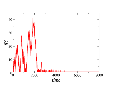
Figure 1: Time evolution of the number of peering links for the unilateral case with cost parameter $\alpha=1$. After a certain equilibration period enforced by our stochastic algorithm, $|P|=1$ is reached.

That said, we would like to make a cautionary note in this regard. The rate of degeneration for $\varepsilon$ must be less than the slowest rate of convergence to equilibrium for the unperturbed process kandori , which makes large state spaces difficult to search. The size of the state space in our game is upperbounded by $2^{|E|}$ where $|E|=|A|^{2}$, given $A$ and $B$ are topologically the same. Even so, simulations on graphs with as many as $100$ nodes indicate that the qualitative relations between parameters observed on smaller graphs remain the same, suggesting the efficacy of the algorithm on larger graphs (as well as the invariance of our results to topological peculiarities).

We numerically simulate the unique limiting stationary distribution of the perturbed dynamic process by the following simple rule:

$$\varepsilon^{t}=\left\{\begin{array}[]{c}0.5\qquad\text{for}\qquad t<10000,\\ 0.5\cdot e^{0.0001(10000-t)}\qquad\text{otherwise.}\end{array}\right.$$ (8)

III Results

In this section we present some simulation results providing a partial characterization of stochastically stable peering configurations when $A$ and $B$ are scale-free networks with $100$ nodes constructed according to the model based on growth and preferential attachment barabasi . It is well known that the topology of large ASes is closely scale-free.

III.1 The unilateral case

Fig. 1 shows the time evolution of the number of peering links for the case where $\alpha=1$ and $\beta=0$ (unilateral flow). The fact that quite many peering links are established for $t\lesssim 3000$ is due to the perturbed dynamic process. As far as the equilibrium state is concerned, we found $|P|_{\text{eq}}=1$ for $\alpha<1$ and in the case $\alpha=1$, there was a $2\%$ chance of ending up with 2 final peering links.

When it comes to the costs, the receiver has to pay an amount of 0.3565 units independently of where the link is established. This has to do with the fixed topology and with the fact that the receiver ($B$) sends no packets in the present case. Concerning the sender, on the other hand, certain nodes are preferable to others in that the incurred traffic costs is lower. Fig. 2 shows the sender’s cost distribution in the stationary state.

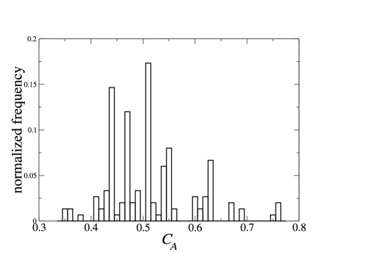
Figure 2: Distribution of the sender’s cost in the steady state (for unilateral flow). This result was obtained by statistically analyzing the costs of graph $A$ for times $10000<t<100000$ for 150 different runs.

III.2 Bilateral flow

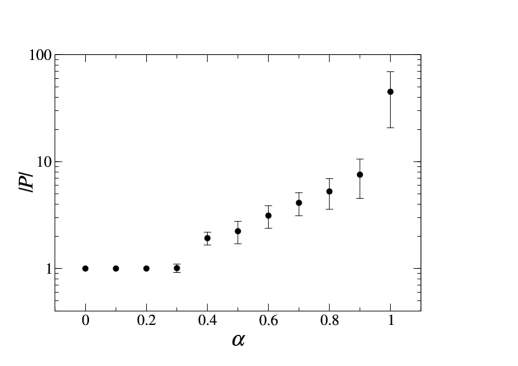
Figure 3: The average number of established peering links as a function of $\alpha$ for the bilateral case. For $\alpha\leq 0.2$ only one link remained in equilibrium, hence the lack of the error bar. Up to $\alpha\leq 0.9$ the distributions were well peaked around the corresponding mean values whereas the present average values were scattered much more broadly for $\alpha=1$ (note the logarithmic scale). These results were obtained for times $10000<t<100000$ and for 150 different runs.

A more interesting situation arises when both ISPs $A$ and $B$ send data packets. We investigated the case where each node in graph $X$ sends one packet to every node in graph $Y$, $X,Y\in\{A,B\}$, i.e. $\beta=1$. Fig. 3 shows the average number of peering links that were established in equilibrium. For $\alpha\leq 0.9$, these values are meaningful quantities as the accompanying variances appear to be small. Note also the exponential growth in the range $0.5\leq\alpha\leq 0.9$. In the case where the peering links no longer contribute to the cost ($\alpha=1$), the peering structure is subject to much stronger fluctuations. In other words, there seems to be some type of phase transition for $\alpha\rightarrow 1^{-}$.

Fig. 4 illustrates the mean values of the costs as $\alpha$ is varied. The fact that $C_{A}$ behaves very similarly to $C_{B}$ is a reflection of $\beta=1$. A rather linear relationship between $C$ and $\alpha$ can furthermore be observed for $\alpha\lesssim 0.8$.

III.3 Ongoing work

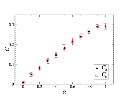
Figure 4: $A$ and $B$’s costs (their averages) as a function of $\alpha$ for $\beta=1$. Note that the costs end up in well defined ranges, and the linear growth with $\alpha$ can be observed as well. For simulational details, see Fig. 3.

We are currently analyzing the equilibria of our game on smaller and more regular, i.e. more tractable, topologies. Initial findings suggest that many efficient peering configurations are pairwise stable over small ranges of $\alpha$ but only stable for a very precise $\beta$. Moreover, we note that the set of pairwise stable configurations contain closely efficient graphs for a broad range of $\alpha,\beta$ pairs. Furthermore, for $\beta=1$ the system exhibits a wide range of stochastically pairwise stable peering configurations for intermediate values of $\alpha$. However, for $\beta<1$, there is a drastic paucity of stochastically stable equilibria and the more efficient peering configurations are no longer stable. This suggests that peering is sensitive to asymmetries, particularly in perceived traffic load distributions. This also means that peering relations are more sensitive to differences in traffic loads than to differences in network size–the latter representing a variation in $\alpha$ as opposed to $\beta$. Of mention is that these results are irrespective of network topology. We are currently working toward a full characterization of stable and efficient configurations in our game.

IV Conclusions

We study how economic incentives affect the peering relationship between two network providers. Specifically, we consider a game where two selfish network providers must establish peering points between their respective network graphs, given knowledge of traffic conditions and a nearest-exit routing policy for out-going traffic, as well as costs based on congestion and peering connectivity involving a parameter $\alpha$ which gives their relative importance. We focus on the pairwise stability equilibrium concept and use a stochastic procedure to solve for the stochastically pairwise stable configurations.

We note a paucity of stochastically stable peering configurations under asymmetric conditions, particularly to unequal interdomain traffic flow, with adverse effects on system-wide efficiency. The volatility of peering relationships in the face of perceived asymetries suggests that peering will become increasingly rare as traffic and cost monitoring become more accurate and available.

For the case of equally bilateral traffic flow, we find a transition in behavior for $\alpha\rightarrow 1^{-}$, meaning that below this value, the number of peering links is well peaked around some mean value and above it, strong fluctuations are observed. We furthermore find that the costs of both providers grow linearly with $\alpha$.

- (1) W.B. Norton. Internet Service Providers and Peering. Equinix White Papers (2001).
- (2) N. Badasyan and S. Chakrabarti. Intra-backbone and Inter-backbone Peering Among Internet Service Providers. e-print ewp-io/0407004 (2004).
- (3) S.-J. Shin and M. Weiss. Internet Interconnection Economic Model and its Analysis: Peering and Settlement. Netnomics 6, 43 (2004).
- (4) R. Johari and J.N. Tsitsiklis. Routing and Peering in a Competitive Internet. Technical Report P-2570, MIT Laboratory for Information and Decision Systems (2003).
- (5) R. Johari, S. Mannor and J.N. Tsitsiklis. A Contract-Based Model for Directed Network Formation. Submitted to Games and Economic Behavior (2003).
- (6) M.O. Jackson and A. Wolinsky. A Strategic Model of Social and Economic Networks. J. Econ. Th. 71, 44 (1996).
- (7) M.O. Jackson and A. Watts. The Evolution of Social and Economic Networks. J. Econ. Th. 106, 265 (2002).
- (8) S. Chakrabarti. Middlemen in Peer-to-Peer Networks: Stability and Efficiency. Proceedings of the 2nd Workshop on the Economics of Peer-to-Peer Systems, Harvard University, Boston MA (2004).
- (9) M.R. Garey and D.S. Johnson. Computers and Intractability. W.H. Freeman and Co., New York (1979).
- (10) M. Kandori, G.J. Mailath and R. Rob. Learning, Mutation, and Long Run Equilibria in Games. Econometrica 61, 29 (1993).
- (11) H.P. Young. The Evolution of Conventions. Econometrica 61, 57 (1993).
- (12) M.I. Freidlin and A.D. Wentzell. Random Perturbations of Dynamical Systems. Springer, New York (1998).
- (13) J. Harsanyi and R. Selten. A General Theory of Equilibrium in Games. MIT Press, Cambridge MA (1988).
- (14) A.-L. Barabási and R. Albert. Emergence of Scaling in Random Networks. Science 286, 509 (1999).