Fast Query Processing by Distributing an Index over CPU Caches

Abstract

Data intensive applications on clusters often require requests quickly be sent to the node managing the desired data. In many applications, one must look through a sorted tree structure to determine the responsible node for accessing or storing the data. Examples include object tracking in sensor networks, packet routing over the internet, request processing in publish-subscribe middleware, and query processing in database systems. When the tree structure is larger than the CPU cache, the standard implementation potentially incurs many cache misses for each lookup; one cache miss at each successive level of the tree. As the CPU-RAM gap grows, this performance degradation will only become worse in the future.

We propose a solution that takes advantage of the growing speed of local area networks for clusters. We split the sorted tree structure among the nodes of the cluster. We assume that the structure will fit inside the aggregation of the CPU caches of the entire cluster. We then send a word over the network (as part of a larger packet containing other words) in order to examine the tree structure in another node’s CPU cache. We show that this is often faster than the standard solution, which locally incurs multiple cache misses while accessing each successive level of the tree.

The principle is demonstrated with a cluster configured with Pentium III nodes connected with a Myrinet network. The new approach is shown to be 50% faster on this current cluster. In the future, the new approach is expected to have a still greater advantage as networks grow in speed, and as cache lines grow in length (greater cache miss penalty). This can be used to successfully overcome the inherent memory latency associated with cache misses.

1 Introduction

In the past decade, hardware technology had two trends. On the one hand, microprocessor speeds have followed Moore’s Law [10], doubling every eighteen months. In the future, we may instead see a doubling of the number of processors per chip, such as multicore/multiprocessor chips, but the effect on computational power is the same. However, the development of memory shows a different trend. Although memory capacity and prices are keeping up with the increase rate of CPU speed, memory latency has improved little. Memory latency for random access to a RAM chip runs into a fundamental lower bound determined by the time to precharge the chip buffer from internal voltages to the voltages needed to drive an external bus. Hence, newer memory standards, such as DDR2 RAM and Rambus RAM, concentrate on improving memory bandwidth, but not memory latency. Over the past decade, the gap between CPU speed and memory latency has increased exponentially. Current technology trends (especially the higher memory pressures due to the introduction of dual and quad processor CPU cores) portend further increases in this gap.

This CPU-memory gap represents a fundamental bottleneck in distributed applications that require messages or queries to quickly be routed to appropriate nodes, based on a large index data structure. Two examples of such an index data structure are a sorted n-ary tree and a sorted array. In the case of the sorted array, one can look up an index via binary search.

We do not consider hash arrays for the index data structure. Specifically, we assume that a key is part of a very large ordered index set. The range of all possible indices is divided into sub-ranges. For example, if the indices have values from 0.0 to 1.0, then there might be three nodes in charge of indices from 0.0 to 0.33, from 0.33 to 0.67, and from 0.67 to 1.0, respectively. In this simple example, the index data structure would record the delimiters 0.0, 0.33, 0.67 and 1.0. The key specified by an incoming query could be any number between 0.0 and 1.0.

We also assume that multiple nodes are available for passing external queries to the correct node, based on the key value in the incoming query. The key must be looked up in the index. We further assume that the index is too large to fit in the CPU cache, and overflows into main RAM. Examples include tracing objects in sensor networks, routing packets over internet, routing requests in publish-subscribe middleware, and query processing with database indices.

In this situation, rather than replicate the index on each node, we propose to distribute the index among the CPU caches of the multiple nodes. We assume that the aggregate CPU cache of the multiple nodes is sufficient to hold the index. We consider three variations of this idea.

We compare each of them with two standard methods (here called Method A and Method B). Methods A and B each duplicate the index structure on each node, accept queries at a single dispatcher node which dispatches queries to an appropriate node according to a load balancing algorithm, and each other nodes lookup the duplicated index structure in memory and dispatch the results to the target. The three variations of Method C have only one copy of the index structure among all the nodes, accept queries on a single master node. The master node passes the query to an appropriate slave node according to one piece of index structure stored on it, then each slave node processes the queries over one piece of index stored on it and dispatches the results to the target. For all methods, the $n$ in an n-ary tree is chosen so that $n$ keys ($n$ 4-byte words in our case) and the corresponding pointers fit exactly in an L2 cache line.

• Method A — index is a large n-ary tree and is duplicated on each node; at each node, each query incurs multiple cache misses.

• Method B — index is a large n-ary tree and is duplicated on each node; at each node, many queries are stored and then processed as a batch; to process a batch of queries, a single pass through the tree is made with a buffering access technique using the L2 cache (see Section 3.1).

• Method C — index is a large sorted array and is partitioned among the nodes; with each slave node holding one partition. The master node holds the delimiters for the partitions.

  • Method C-1 — the partition on the slave node is stored as an n-ary tree.

  • Method C-2 — the partition on the slave node is stored as an n-ary tree; As with Method B, queries are stored and processed in a batch. To process a batch of queries, a single pass through the tree is made with the buffering access technique, but using the L1 cache instead of the L2 cache (see Section 3.2).

  • Method C-3 — the partition on the slave node is stored as a sorted array.

Method C is the novel method of distributed in-cache index (based on aggregating the CPU cache from multiple nodes). The distributed in-cache index is formally defined in Section 2, and contrasted to traditional cooperative caching (based on aggregating the RAM from multiple nodes). Method B is based on the buffering access technique, described by Zhou and Ross [14]. Section 3 describes all of the methods studied here. In the experimental section (Section 4.1), we demonstrate that Method C-3 is the best for simultaneously satisfying the two criteria of throughput and response time.

Modeling the Future. Although Method C-3 is somewhat faster today, it is important to demonstrate that the advantage of Method C-3 will widen further in the future. This is important as CPU speed, memory bandwidth, and network speed all increase. In order to predict the speeds of the five methods using future technology, we first define a simple analytical model that successfully analyzes the running time of the five methods on today’s architecture. Our analytical models are based on architectural parameters of the technology employed.

The analytical model was first checked for accuracy against the Methods A, B and C-3. (Methods C-1 and C-2 could also be analyzed, but current experiments showed them to be inferior to C-3.) The analytical model was found to be accurate within 25% for the three methods analyzed.

We then make reasonable assumptions about technology trends, in order to plug in architectural parameters for future technologies. Appendix A describes the analytical model that predicts the performance of the three methods. Section 4.2 demonstrates future trends of the three methods based on the model.

1.1 Related Work

The concept of the memory wall has been popularized by Wulf [13]. Many researchers have been working on improving cache efficiency to overcome the memory wall problem. The pioneering work [9] done by Lam et al. has both theoretically and experimentally studied the blocking technique and described the factors that affect the cache formance. However, there is not an easy way to apply the blocking technique to the tree traversal problem or to the index structure lookup problem to improve the cache efficiency.

The issue of cache and n-ary trees is closely related to the issue of memory-resident B+-trees. There is a large stream of research on this in the database community  [3, 5, 7, 12, 14]. Rao [12] proposed the CSB+ tree (cache sensitive B+ tree). In a CSB+ tree, the branching factor is improved by storing only the first child pointer at each node. Other child pointers can be calculated by adding the offset to the first child pointer because all child nodes are stored consecutively in the memory space in a CSB+ tree. Recently, Zhou [14] proposed the buffering access technique to improve the cache performance for a bulk lookup. However, cache miss penalties still account for over 30% of the total cost for each query in all above proposed methods.

In the area of theory and experimental algorithms, Ladner et al. [8] proposed an analytical model to predict the cache performance. In their model, they assume all nodes in a tree are accessed uniformly. This model is not accurate for the tree lookup problem. Because the number of nodes from root node to leaf nodes is exponentially increasing, nodes’ access rates are exponentially decreasing as the their positioned levels in the tree increase. Hankins and Patel [7] proposed a model with an exponential distributed node access rate in a B+ tree according to the level of a node positioned. However, they only considered the compulsory cache misses, and not the capacity cache misses. They also assume that the tree can fit in the cache. So, for tree structures that can’t fit in the cache, the model in [7] is not applicable.

With the development of the technologies, the performance gap between sequential and random accesses to RAM is increasing due to difficulties in circuit design, such as the issue of precharging the buffer. Cooperman et al. [4] studied the performance impact of random accesses to RAM and proposed the MBRAM model that distinguishes between random and sequential accesses to RAM. They also show that tree traversal applications can generate many random memory accesses resulting in degraded performance, as demonstrated by heap sort. In parallel, Byna et al. [2] proposed a memory cost model for looping operations.

2 Distributed in-Cache indices

2.1 The Definition of Distributed in-Cache Indices

Historically, one often used aggregate memory in a cluster to store files to reduce the number of disk accesses. We explore the use of this technique one level higher in the memory hierarchy than what is traditionally considered to avoid random memory accesses. Because a large index will not fit in cache, we will partition the index among the caches of the many nodes in a cluster. We call this a distributed in-cache index.

We design a more effective index lookup strategy over the distributed in-cache index. The following technology trends stimulate us to distribute an index over CPU caches in a cluster:

1. The disparity between processor speed and memory speed is increasing. As we move to faster, multiple-core CPU chips, the aggregate processor performance is increasing much more rapidly than main memory (RAM) performance. This divergence makes it increasingly important to reduce the number of memory accesses, especially random memory accesses. Index lookup and tree traversal problems produce many random memory accesses. For instance, in the Pentium 4, the L2 cache miss penalty is around 150 ns, which will waste more than 200 CPU cycles of modern microprocessors.

2. Emerging high-speed low-latency switched networks can transfer data across the network much faster than standard Ethernet. The combined cost of index lookup in the remote L2 cache and data transfer over an older network might be more expensive than the cost of index lookup in the local memory. With today’s high-speed low-latency networks, the cost of data transfer in a batch over the network is lower than the cost of many random accesses to local memory, due to the stagnating performance of RAM with respect to memory latency in recent years. For example, on the Boston University Linux cluster, the measured random memory bandwidth for a series of 4-byte word accesses at random locations is 48 MB/s (where each such random access typically incurs a cache miss), although the sequential memory bandwidth (accessing words in sequence) is 647 MB/s. The measured one-way Myrinet bandwidth is 1.1 Gb/s (or 138 MB/s) which is much faster than the random memory bandwidth. Further more, in most of today’s systems, communication can overlap with computation. This makes the communication cost negligible.

2.2 Design Issues for Distributed in-Cache Indices

Network latency:

Local area network latencies range from the extremely short latency of Myrinet (approximately 7 $\mu$s) to latencies of about 100 $\mu$s for Gigabit Ethernet. (Further, depending on the protocol stack of the operating system, the latency seen by the application may be much worse.) By aggregating many queries into larger, batched network messages, we can amortize the latency over the transimission time. In Myrinet (which is used in our experiments), the transmision time for a 10 KB message (about 10 KB/(1.1 Gb/s) = 80 $\mu$s) clearly dominates the latency (7 $\mu$s). For Gigabit Ethernet, one may need to batch a message as large as 200 KB for the transmission time to dominate the latency, but the same principle applies.

Memory bandwidth:

The memory bandwidth of DDR-266 RAM is 2.1 GB/s, and still faster variations are available today. Hence, the full bandwidth of RAM is faster than the network.

Memory latency:

For random memory accesses, memory latency will dominate if not handled appropriately. On the Pentium III, a cache miss for a 4-byte word will require a 32 byte cache line to be loaded. Hence, the effective memory bandwidth degrades by at least a factor of 8. (In fact, the precharging delay of DRAM technology increases the degradation factor.) The Pentium 4 has a 128 byte cache line, with a corresponding degradation factor of 32 in the worse case when successively accessing words are on different cache lines. (In this random access pattern, each access of a four-byte word requires loading a new cache line of length 4$\times$32 bytes.)

CPU time:

We can neglect the CPU time in modeling the overall time for applications with intensive memory accesses. This is because CPU computation and memory access are overlapped, and memory access time greatly dominates over the time for today’s very fast CPUs.

Cache Contention:

We assume that the aggregate cache size across all CPUs is sufficient to hold the distributed in-cache index. As a message of batched queries is loaded, this will lead to cache pollution by evicting some portion of the index. However, the effect of cache pollution is limited. For a 4-byte query key, a single cache line of queries will hold 8 keys on the Pentium III (and 32 keys on the Pentium 4). Assuming that query key values are random, each of the 8 queries will access one leaf node in the index. Hence, for each cache line of queries that is processed, we will refresh at least 8 different cache lines of the tree. The effect is larger when one considers interior nodes of the tree. Further, the Pentium 4 raises this factor from 8 to 32. Hence, to the extent that a cache eviction algorithm approximates an LRU algorithm, the probability of evicting a cache line containing query keys is much larger than the probability of evicting a cache line containing a part of the index.

3 Different Index Lookup Methods in a Distributed Environment

The introduction provided an overview of Methods A, B and C. Method C in fact consists of three submethods, C-1, C-2, and C-3. Method A is a straightforward lookup in a sorted n-ary tree, each node has a replication of the complete tree. In Method B, each node also has a replication of the complete tree, but its description is more complicated. We describe Method B, followed by Method C.

3.1 Method B

Method B is based on an idea of Zhou and Ross [14]. They proposed the buffering access method for a stream of arriving search keys, as shown in Figure 1.

The index tree is logically decomposed into several subtrees. A subtree consists of a root node and all of its descendants, down to some level $k$, where $k$ is chosen so that the subtree tree will fit in the L2 cache. Along with each subtree, the algorithm maintains an associated buffer to store search keys that reach the root node of the subtree.

The key to the success of Method B is to process a batch of search keys at the same time. Each key $k$ in the batch is looked up in the top level subtree. The search within the top level subtree will lead to a leaf node, $x$, of that subtree. The node $x$ is also the root of a lower subtree. The key $k$ is then stored into the buffer associated with the subtree rooted at $x$.

If there are $\ell$ leaf nodes in the top level subtree, then this requires streaming write access to $\ell$ buffers. For $\ell$ of reasonable size, this process is efficient.

Figure 1: Buffering Access Method

After the top level subtree has been processed, each lower subtree is processed using the keys stored in its buffer as the batch of search keys. And so the algorithm proceeds recursively.

Since a subtree and its associated buffer can fit inside the L2 cache, the process is fast, aside from the need to write to different buffers. Since the write access is a streaming access, it avoids the high latency overhead of a cache miss. Further, such writes can be non-blocking.

3.2 Method C

Method C is the proposed new method of Distributed in-Cache indices. Unlike Method B, the new method intrinsically requires many nodes. It assumes that a single node of our architecture is distinguished as the master node, and the rest are slave nodes. Queries always arrive at the master node, which dispatches them to the slave nodes.

The sorted array is decomposed into equal size partitions and each partition is stored at a slave node in the cluster. We assume that each partition fits in the CPU cache. We further assume that there are sufficient nodes to hold these cache-sized partitions.

Next, the master node contains a data structure used to determine to which slave node the query should be dispatched. We used a sorted array of partition delimiters on the master node to determine to which child a query should be passed. This is illustrated in Figure 2.

Figure 2: Cooperative Caching Design

The submethods C-1, C-2 and C-3 are distinguished according to how the slave node does the key lookup. In method C-1, the slave node stores its part of the index as an n-ary tree. An optimization of Rao and Ross [12] is used to store one pointer at each node of the tree. Given a node, its children in a tree are stored at adjacent locations. Hence, it suffices to store only a pointer to the first child of a node. (Rao and Ross gave this data structure the name CSB+ tree.)

Method C-2 adds to this optimization by employing the buffered access proposed by Zhou et al. [14], described earlier for Method B. That is, the partition on a slave node is divided into subtrees, such that each subtree can now fit inside the L1 cache.

Method C-3 employs a simple sorted array. It employs binary search for key lookup.

Remark. In principle, if there is a heavy load of incoming queries, a single master node could become overloaded. This is easily remedied by setting up multiple master nodes, with replicates of the top level data structure.

4 Experimental Validation

We did all experiments on a Pentium III Linux cluster (Red Hat release 7.2). There are 54 nodes on the Linux cluster. Each node has two 1.3 GHz Pentium III processors sharing 1 GB of memory. Each processor has its own 16 KB L1 cache and 512 KB L2 cache. The cluster has two choices of network interconnect: a 100 Megabit/second Ethernet and Myricom’s 2.2 Gigabit/second Myrinet. For communication, we use the MPICH 1.2.5 [11] implementation of MPI [6]. The default network interconnect for MPI is the 2.2 Gigabits/second Myrinet with the GM protocol. All programs are compiled with $mpiCC$ using the $gcc-3.3.1$ compiler with optimization level O3.

We measured the one-way bandwidth of Myrinet as 1.1 Gb/s or 138 MB/s. The measured memory bandwidth (Pentium III, 266 MHz DDR RAM) was 647 MB/s for sequential memory access, and was 48 MB/s for random memory access (random access to a 4 byte word).

Note that since Method A incurs many cache misses, the memory bandwidth that it experiences is actually closer to the 48 MB/s quoted above. This is slower than the network bandwidth 138 MB/s of Myrinet, and helps explain the experimental results.

The parameters for the tree structure used in all experiments are reported in Table 1 except where specifically explained. Both the search keys and the keys used to construct the index structure are randomly generated.

For Methods A and B, the node size in the tree structure is equal to the L2 cache line size. For Methods C-1 and C-3, the node size in the tree structure is equal to the L1 cache line size. In Pentium III, both the L1 cache line size and L2 cache line size are 32 bytes. For Method C-2, the node size is set to half size of the L1 cache to fit in the L1 cache and assistant the buffering technique. In the implementation, the search key and the corresponding lookup result are stored in the same memory location to lessen the cache contention.

Number Of Keys On The Sorted Array	327 kilo
Search Key Size	4 bytes
Index Tree Size	3.2 MB
Subtree Size (except the root subtree) (in B, C)	320 KB
Root Subtree Size (in B, C)	44 bytes
T (in A, B)	7
L (in C-1, C-2)	6
Size of Node (in A, B, and C-1)	32 bytes
Size of Root Node (in C-2)	32 bytes
Size of Leaf Node (in C-2)	8 KB

Table 1: The Index Structure Setup

4.1 Comparing Methods A, B and C

In all experiments, the index tree described in Table 1 is applied. We generate 8 million ($2^{23}$) random search keys. We use 11 nodes. For methods A and B, the 8 million search keys are looked up locally on one node. For method C, one of the 11 nodes acts as the master, and the others act as slaves.

Hence, for method C to be competitive, it must process a search key 11 times faster than for method A and method B (since methods A and B can use all 11 nodes, operating in parallel). This is in fact the case, as will be seen in Figure 3. In order to make for a fair comparison, normalization is applied to methods A and B: the running time measured for a query using method A or B is divided by 11.

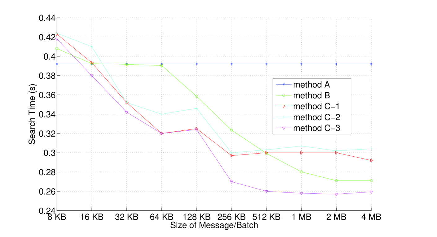
Figure 3: Comparing Method A, B, and C: 8 million ($2^{23}$) search keys (32 MB) over 11 nodes

In Figure 3, the x-axis shows the increase of the batch size. The y-axis shows the running time for 8 million search keys. We did experiments for batch sizes ranging from 8 KB to 4 MB. In practice, one doesn’t need to batch up to 4 MB. Here we just want to show the performance trends with increasing batch sizes. In Figure 3, , one can see that the performance doesn’t change when the batch sizes are larger than 512 KB.

Note also that this experimental comparison gives the benefit of doubt to Methods A and B. With 11 nodes to process queries, Methods A and B require a load balancing algorithm to evenly distribute incoming queries among all nodes. Method C does not require load balancing, since all queries arrive at a single master node before being dispatched. In this comparison, the overhead of load balancing is assumed to be zero.

Even after handicapping Method C by not charging overhead for Methods A and B, all of the experiments show that Method C-3 has the best performance. Further, this holds according to either of two distinct measures: throughput or response time. The advantage of Method C-3 with respect to throughput is self-evident from the figure.

Figure 3 also demonstrates the faster response time of Method C-3 over Method B. We take, as an example, the situation when a fixed throughput of 8 million search keys in 0.32 seconds must be processed. The figure shows that Methods C-2 and C-3 achieve this throughput with a batch size of only 64 KB, while Method B requires a batch size of 256 KB to achieve that same search time. (Of course, Method A has a much faster response time, since it processes search keys individually. However, our point is that Method C is capable of simultaneously satisfying severe constraints in both throughput and response time.)

Methods C-1 and C-2 follows the same trend as Method C-3 with the increasing batch sizes, but they tend to have a slightly worse performance. This is because the n-ary trees of Methods C-1 and C-2 occupy more space than a sorted array. This produces more pressure on the cache.

From Figure 3, we see that the Methods C are significantly faster even for the relatively small batch sizes of 32 KB and 64 KB. We observe a 22% reduction in run time with this configuration. For very large batch size, performance improvement can still be observed even without cache coloring. If a batch size is 16 KB or less, Methods C-1, C-2, and C-3 are worse than method B and method A.

For a batch size of 8 KB, there are 1,000 messages, with an aggregate communication latency of $1000\times 7$ $\mu$s. The overhead for 8 KB is small, and for larger batch sizes (fewer messages), the overhead is negligible.

In the experiments, we also observed that slaves were idle for 50% of the time for 8 KB batch sizes, and 20% of the time for 4 MB. We attribute this overhead both to the overhead of MPI and the operating system, and statistically varying load balance among the slave nodes. This per-message overhead is amortized across more queries as the message size increases. Messages were sent using MPI_Isend in order to overlap computation and communication to the extent supported by the hardware.

The performance degrades slightly as the message size is increased from 64 KB to 128 KB. We attribute this to cache contention. When message sizes are 128 KB, the cache will see the 128 KB of query lookups for the current message, 128 KB of the next message of queries being received (overlapped communication and computation), and a 320 KB subtree for the local partition of the index. This adds to more than the 512 KB size of the L2 cache on the Pentium III.

When the batch size rises beyond 128 KB, the presure of L2 cache contention will be the same. In that range, the benefit of the lower slave idle time will overcome the penalty due to cache contention, and boost the overall performance.

Our choice of 8 million search keys is for the purpose of demonstrating the trend for larger batch sizes. Pragmatically, one would choose a smaller batch size for its improved response time, while achieving similar throughput.

4.2 Predicting the Future

Our initial goal was to define an analytical model accurate enough to predict the present experimental results. For this purpose, we wrote programs to measure the environment parameters of the Linux cluster. We measured the memory bandwidth, network bandwidth, L2 cache line miss penalty, L1 cache line miss penalty, comparison cost at a node whose size is equal to the L2 cache line size. These numbers are reported in Table 2, and were used in the analytical model (described in the Appendix).

Using the measured parameters and the equations in Appendix A, the average cost for a query with three different methods is predicted. These are reported in Table 3. We also did experiments to show the accuracy of our evaluation. In Table 3, the batch size equal to 128 KB is applied, and one master and ten slaves are used in method C. For fair comparison, normalization that the total running times for Methods A and B are divided by 11 is applied. Table 3 shows that our model has over 90% of accuracy.

Parameter	Value
L2 Cache Size	512 KB
L1 Cache Size	16 KB
L2 Cache line Size	32 bytes
L1 Cache line Size	32 bytes
$B_{2}\_Miss\_Penalty$	110 ns
$B_{1}\_Miss\_Penalty$	16.25 ns
TLB Entries	64
$Comp\_Cost\_Node$	30 ns
$W_{1}$ (Memory Bandwidth)	647 MB/s
$W_{2}$ (Network Bandwidth)	138 MB/s

Table 2: Parameters On the Linux Cluster

Strategy	Equation	predicted	experimental
		time	time
Method A:	Equation A.2.1	0.45 s	0.39 s
Method B:	Equation A.2.2	0.38 s	0.36 s
Method C-3:	Equation A.2.3	0.28 s	0.32 s

Table 3: Normalized Predicted and Experimental Running Time for 8 Meg ($2^{23}$) keys

Table 3 provides assurance that the model is reasonably accurate (at least to within 25%). With confidence in our present-day estimates, we go on to predict the future.

We assume that CPU speed will continue to double every 18 months, while network speed will double only every 3 years. Memory bandwidth is assumed to grow, but the number of processors sharing the same memory bandwidth may grow also with the trend to multi-processor CPU chips. We assume the memory bandwidth available for one processor will grow 20% per year. Memory latency is assumed not to change.

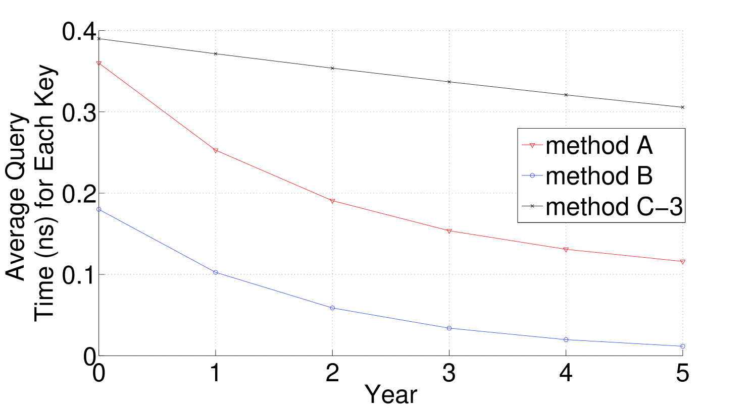
Figure 4: Future Trends Based on Model (128 KB batch size, 8 meg ($2^{23}$) keys)

Looking into the future. We next employ highly approximate techniques to argue the trends in the future. We do not claim high accuracy for this speculative section. However, even this crude argument will suffice to argue the trends.

Figure 4 demonstrates that the advantage of Method C-3 will continue to grow. Note that the ratio of times comparing Method B to C-3 grows from approximately a factor of 2 in year 0 to about a factor of 10 in year 5. Methods C-1 and C-2 were not graphed, for simplicity, but their curves would be close to that of C-3.

There is clearly some inaccuracy both in our analytical model as compared to experiment, and in our assumptions of future trends. Nevertheless, the trend of a growing speed advantage for Method C-3 is strong, and the conclusion is likely to remain under other scenarios of future technological trends.

5 Conclusion

We proposed and evaluated the distributed in-cache indices for the tree lookup problem. The experiments show all methods (C-1, C-2, and C-3) with distributed in-cache indices outperform other methods when combing the two worlds, throughput and response time. Especially, Method C-3 is the best in most scenario. Method C-3 is two times faster than Method A and has much higher throughput and faster response time than Method B. Our analytical model argues that technological trends of faster CPU and network will further favor Method C-3.

6 Acknowledgment

We thank the Mariner Project at Boston University for providing the experimental facilities.

Appendix A APPENDIX: Analysis of Index Lookup for the Three Methods

We introduce a model to analyze the cache performance of a tree index structure. The model is based on the expected number of cache line misses for each key lookup. TLB misses are not considered in our model. So our model gives a lower bound for the running time. Then we apply this model to analyze three different designs.

In our model, an n-ary tree index structure and a stream of arriving search keys are assumed. The variable $n$ is chosen so that $n$ computer words fit in an L2 cache line.

Table 4, below, enumerates all the notations that will be used in our later discussion:

variable	Description
$Tree\_Size$	the size of the B+ tree
$T$	the total levels of the B+ tree. $T=(log(M/K)/log(K+1)+1)$
$L$	the levels of the B+ tree can fit in cache. Each slave hold $L$ levels of the B+ tree
$W_{1}$	the memory bandwidth 647 MB/s
$W_{2}$	the network bandwidth 138 MB/s
$C_{2}$	the size of L2 cache
$B_{2}\_Miss\_Penalty$	the cost of loading a cache line from the memory to the L2 cache
$B_{2}$	the size of the L2 cache line in bytes
$B_{1}\_Miss\_Penalty$	the cost of loading a cache line from the L2 cache to L1 cache
$B_{1}$	the size of the L1 cache line in bytes
$Comp\_Cost\_Node$	the cost to traverse one level of the B+ tree while searching a key
$NUM_{masters}$	the number of master nodes
$NUM_{slaves}$	the number of slave nodes that have lower L levels of the B+ tree in L2 cache
$NUM_{keys\_per\_batch}$	the number of search keys in one batch lookup

Table 4: Parameters Used in The Model

A.1 The Model of Cache Performance for Tree Traversal

We follow the analysis of Hankins and Patel [7]. They assumed that the probability of accessing a vertex in a tree depended on its level in the tree. Hence, for an n-ary tree, the children of the root node have probability of being accessed on the next round that is 1/n of the probability of the root node being accessed next.

According to [7], for a tree that can fit in the L2 cache, the expected number of cache misses for each key lookup is:

$$\frac{\sum_{i=1}^{T}X_{D}(\lambda_{i},q)}{q}$$ (1)

where:

$$X_{D}(\lambda_{i},q)=\lambda_{\times}(1-(1-1/\lambda_{i})^{q})\\$$ (2)

In the above formula, $\lambda_{i}$ is the number of cache lines at the $i$th level of the tree, $q$ is the total number of keys to be lookuped.

We use [7] as the foundation and further explore the model. We analyze the problem in two steps:

1. We assume that the tree space touched by the first $q_{0}$ lookups is exactly the size of L2 cache. The cache state is marked as the state $S0$. The state $S0$ represents a state when all of the cache has become occupied by the tree structure.

   $$\sum_{i=1}^{T}X_{D}(\lambda_{i},q_{0})=C_{2}/B_{2}$$ (3)

2. The number of caches misses for each key lookup after the $q_{0}$th lookup is:

   $$\sum_{i=1}^{T}X_{D}(\lambda_{i},q_{0}+1)-\sum_{i=1}^{T}X_{D}(\lambda_{i},q_{0})=$$ (5)

   $$\sum_{i=1}^{T}X_{D}(\lambda_{i},q_{0}+1)-C_{2}/B_{2}\mbox{\hskip 72.26999pt}$$

   For the $(q_{0}+1)$-th lookup, the amount of space loaded from memory to cache is calculated by Equation 5. After the $(q_{0}+1)$th lookup, the cache state is same as the state of $S0$. Hence, for all later lookups, each lookup needs to load the space (calculated in Equation 5) from memory to cache.

A.2 Index Structure Analysis for Search Operands

In our evaluation, we examine only the data cache behavior, while ignoring the instruction cache misses and TLB misses. Instruction cache performance is ignored, because the instruction complexity is comparable between three methods. Method A and method B are significantly affected by TLB misses, because they work on very large datasets. In contrast, method C generates few TLB misses, except immediately after a cold start. This is because Method C works on a small contiguous dataset in memory. Hence, the following analysis results yield a lower bound running time for Methods A and B, but a more accurate running time for Method C.

A.2.1 Method A: Standard Method

For each key lookup the cost for the standard one-by-one key lookup is:

$$T\times Comparison\_Cost\_Node+\frac{8}{W_{1}}+$$

$$(\sum_{i=1}^{T}X_{D}(\lambda_{i},q_{0}+1)-C_{2}/B_{2})\times B_{2}\_Miss\_Penalty$$

The first term is the computation cost and the other terms are the memory access costs.

Any path from the root node to one of the leaf nodes consists of $T$ nodes for a tree with $T$ levels. So, for each search key lookup, the computation cost is $T\times Comparison\_Cost\_Node$.

The memory access cost consists of two parts: buffer access cost and tree access cost. Each search key needs to be read from an input buffer and to be written to an output buffer. The costs of reading from a buffer and writing to a buffer are $4/W_{1}$ each, because the input buffer and output buffer are accessed sequentially.

The tree access cost is calculated according to the equation 5 with $q\gg q0$. We ignore the time spent to access data in the L2 cache, because access to data in memory dominates the time. Intuitively, the frequently accessed upper levels of the tree have higher probability of remaining in cache, but the lower levels of the tree are usually not in the cache. Hence, a cache miss typically happens at each level when accessing the lower parts of the tree.

A.2.2 Method B: The Buffering Access Method

For each search key, the cost is:

$$T\times Comparison\_Cost\_Node+\triangle+ \frac{4}{W_{1}}\times(T/L)+$$

$$\frac{B_{2}\_Miss\_Penalty\times 4}{B_{2}}\times(T/L-1)$$

The first term represents the computation cost explained in Section A.2.1 . The other terms represent memory access costs. The tree access cost is $\triangle$.

The memory access cost to read a key from buffers is $4/W_{1}\times T/L$, because each buffer is sequentially accessed and there are a total of $T/L$ subtrees. The total memory access cost to write a search key to buffers is $\frac{B_{2}\_Miss\_Penalty\times 4}{B_{2}}\times(T/L-1)$, because each time a write buffer is selected according to a random key value.

The tree access cost has two parts: the time spent to load the subtrees from memory to L2 cache one by one ($\theta_{1}$); and the time spent to access the subtree in the L2 cache after a subtree has been loaded into L2 cache ($\theta_{2}$). The time spent to load all the subtrees from memory to L2 cache can be calculated with Equation 1 because each subtree can fit in the L2 cache. For each key lookup, the average number of L2 cache misses are:

$$\theta_{1}=\frac{\sum_{i=1}^{T}X_{D}(\lambda_{i},q)}{q}\times B_{2}\_Miss\_Penalty$$ (6)

For each lookup, the number of nodes to be accessed is $T$ and the number of L2 cache lines to be accessed is also $T$, because the size of node is same as the size of L2 cache line. The number of cache lines to be accessed in the L2 cache will be $T-{\sum_{i=1}^{T}X_{D}(\lambda_{i},q)}/{q}$. Therefore, the time spent to access to data in the L1 cache will be:

$$\theta_{2}=(T-\frac{\sum_{i=1}^{T}X_{D}(\lambda_{i},q)}{q})\times B_{1}\_Miss\_Penalty$$ (7)

A.2.3 Method C: Distributed in-Cache indices for Index Structures

We make the following assumptions, which simplify the analysis.

1. Aggregate network bandwidth is unlimited.

2. There are enough nodes in the cluster so the the aggregate L2 caches over the cluster can hold the entire index structure. Each node does computation and data accesses in cache.

3. $T<2L$, so that each search can be done within the caches of just two nodes: a master and a slave. Here, we make this assumption to make the model simpler. In practice, if $T>2L$, each search needs to traverse more than the caches of two nodes and our design still can be applied.

4. The master and slaves do their tasks in parallel.

For each search key, the average cost is

$$\max\bigg{\{}\frac{Dispatch\_Cost+\frac{8}{W_{1}}+\frac{4}{W_{2}}}{num_{masters}},$$

$$\frac{L\times(Comp\_Cost\_Node+B_{1}\_Miss\_Penalty)}{num_{slaves}}$$

$$+\frac{\frac{8}{W_{1}}+\frac{4}{W_{2}}}{num_{slaves}}\bigg{\}}$$

In Equation A.2.3, the first part is the cost on the master side and the second part is the cost on the slave side. The maximum value is the real cost because masters and slaves do tasks in parallel. The following explains how to calculate the costs on the master side and the slave side.

Cost on the master side for each search key:

1. Computation time: $Dispatch\_Cost\_Per\_Search\_Key$. This cost depends on the distribution of search key values. We assume uniformly distributed search key values.

2. Memory access time: $8/W_{1}$. This cost is to read a key from the search key array and put the key to a buffer for an outgoing message. Because accesses to the search key array and the buffer are both sequential, the full memory bandwidth can be used to transfer data.

3. Communication time: $4/W_{2}$. For each search key, network transmission time is considered, but not latency. This is because keys are sent out in a message with the size given of kilobyte magnitude and larger.

The cost on the slave side for each search key:

1. computation time: $L\times Comparison\_Cost\_Node$. Each slave maintains an $L$-level subtree.

2. memory access time: $8/W_{1}$. Reading a key from an incoming message buffer and writing the result to an outgoing message buffer.

3. communication time: $4/W_{2}$. Sending the search result to the masters. The transmission time is considered, but not latency. This is because results are sent in a message with the size of kilobyte magnitude or larger.

4. L2 access time: $L\times B_{1}\_Miss\_Penalty$. The tree can fit in the L2 cache, but not in the L1 cache. For each search key, at each level a L1 cache miss may happen.

In Section 3.2, we described three alternative designs, C-1, C-2 and C-3. They have similar performance. Equation A.2.3 can be applied to all of them.

References

- [1] A. Ailamaki, D. J. DeWitt, M. D. Hill, and D. A. Wood. DBMSs on a modern processor: Where does time go? In Proc. of Very Large Databases (VLDB), 1999.
- [2] S. Byna, X. Sun, W. Gropp, and R. Thakur. Predicting memory-access cost based on data-access patterns. In IEEE International Conference on Cluster Computing, 2004.
- [3] S. Chen, P. B. Gibbons, T. C. Mowry, and G. Valentin. Fractal prefetching B+-trees: Optimizing both cache and disk performance. In Proc. of SIGMOD, 2002.
- [4] G. Cooperman, X. Ma, and V. H. Nguyen. Static performance evaluation for memory-bound computing: the mbram model. In Proc. of the 2004 International Conference on Parallel and Distributed Processing Techniques and Applications (PDPTA’04), pages 435–441, 2004.
- [5] G. Graefe and P. Larson. B-tree indexes and CPU caches. In Proc. of 17th International Conference on Data Engineering (ICDE), 2002.
- [6] W. Gropp, E. Lusk, and A. Skjellum. Using MPI (2nd edition). MIT Press, 1999.
- [7] R. A. Hankins and J. M. Patel. Effect of node size on the performance of cache-conscious B+-trees. In Proc. of SIGMETRICS, pages 283–294, 2003.
- [8] R. E. Ladner, J. D. Fix, and A. LaMarca. Cache performance analysis of traversals and random accesses. In Proc. of Tenth ACM-SIAM Symposium on Discrete Algorithms, 1999.
- [9] M. Lam, E. Rothberg, and M. Wolf. The cache performance and optimzations of blocked algorithms. In 4th Int. Conf. on Architectural Support for Programming Languages and Operating Systems (ASPLOS IV), pages 63–75, 1991.
- [10] G. Moor. Cramming more components onto integrated circuits. Electronics, 38:114–117, 1965.
- [11] http://www.mcs.anl.gov/mpi/mpich/.
- [12] J. Rao and K. A. Ross. Making B+-trees cache conscious in main memory. In Proc. SIGMOD, pages 475–486, 2000.
- [13] W. Wulf and S. McKee. Hitting the memory wall: Implications of the obvious. ACM Computer Architecture News, 23:20–24, 1995.
- [14] J. Zhou and K. A. Ross. Buffering accesses to memory-resident index structures. In Proc. VLDB, pages 405–416, 2003.