Analysis of and workarounds for element reversal for a finite element-based algorithm for warping triangular and tetrahedral meshes

Abstract

We consider an algorithm called FEMWARP for warping triangular and tetrahedral finite element meshes that computes the warping using the finite element method itself. The algorithm takes as input a two- or three-dimensional domain defined by a boundary mesh (segments in one dimension or triangles in two dimensions) that has a volume mesh (triangles in two dimensions or tetrahedra in three dimensions) in its interior. It also takes as input a prescribed movement of the boundary mesh. It computes as output updated positions of the vertices of the volume mesh. The first step of the algorithm is to determine from the initial mesh a set of local weights for each interior vertex that describes each interior vertex in terms of the positions of its neighbors. These weights are computed using a finite element stiffness matrix. After a boundary transformation is applied, a linear system of equations based upon the weights is solved to determine the final positions of the interior vertices.

The FEMWARP algorithm has been considered in the previous literature (e.g., in a 2001 paper by Baker). FEMWARP has been succesful in computing deformed meshes for certain applications. However, sometimes FEMWARP reverses elements; this is our main concern in this paper. We analyze the causes for this undesirable behavior and propose several techniques to make the method more robust against reversals. The most successful of the proposed methods includes combining FEMWARP with an optimization-based untangler.

1 Introduction

There are numerous applications in science and engineering (and other domains as well) for which the domain of interest deforms as a function of time. These applications include structural anatomical remodeling associated with heart failure helm , traumatic brain injuries darvish , metal forming lee , and fluid flow applications ishikawa (to name just a few). For such applications, the mesh must be updated at each time step in response to the deforming domain boundary, thus resulting in potentially drastically varying mesh quality from step to step. It is well-known that poor quality elements affect the stability, convergence, and accuracy of finite element and other solvers because they result in poorly-conditioned stiffness matrices and poor solution approximation shew_quality . Hence, it is important for the updated meshes to be of reasonable quality, as well.

The specific mesh-updating problem on deforming domains which we study is as follows. Here we follow the description in knupp_dd . Suppose $\Omega$ is an initial undeformed domain and $M$ is an original mesh on $\Omega$. Further, suppose that $M$ is of good quality. Then, suppose the domain deforms due to a change in shape, orientation, volume, etc. Let $\hat{\Omega}$ be the deformed domain. The goal is to create a mesh $\hat{M}$ on $\hat{\Omega}$ that is of reasonable quality. In addition, it is often desired that $\hat{M}$ be ‘similar’ to $M$ in some sense; e.g., we desire that the two meshes have the same topology. Similar meshes are often desired between successive time steps of a physical simulation or between successive iterations of an optimal-design procedure so that the solution varies smoothly between successive deformations.

If one were given an onto map $X(\Omega,t)$ from $\Omega$ to $\hat{\Omega}$ at a specified time $t$, then $\hat{M}$ could be determined by evaluating $X(\Omega,t)$ at the vertices of $M.$ However, for many applications, such a map is not known. In this situation, $\hat{M}$ could be created via an automatic mesh generator. However, this is a computationally intensive process, and the resulting mesh will likely not be similar to $M$. Thus, $\hat{M}$ should be created using a mesh-update procedure. Even if the boundary map between $\Omega$ and $\hat{\Omega}$ is given, the mesh-updating problem is not easy due to the similarity requirement.

Several partial differential equation-based (i.e., PDE-based) approaches for solving the mesh-updating problem in response to a deforming domain boundary, under the assumption that the boundary map, $X(\Omega,t)$ from $\Omega$ onto $\hat{\Omega}$ at time $t$, is specified, have been designed. Work has focused on the development of spring model approaches based on Laplace’s equation, variable diffusion, and biharmonic PDEs for vertex movement helenbrook2003 ; branets2005 ; shontz2003 ; stein2003 . Other research has focused on the development of elasticity-based approaches stein2004 ; tezduyar1992 ; ShontzThesis . Many existing serial and parallel mesh-updating methods baker ; li2001 ; cardoze1 ; cardoze2 ; selwood96parallel ; selwood97parallel ; shephard03automated ; seol06efficient ; antaki00parallel combine vertex movement with other techniques which alter the mesh topology and violate the similarity requirement.

Another important limitation of most mesh-updating approaches is that they can reverse elements during the mesh updating procedure during a given timestep. “Reversal” means that the element changes orientation. In two dimensions, this means that the vertices of an element are clockwise when they ought to be counterclockwise, and in three dimensions it means that they violate the right-hand rule. Meshes with reversed elements yield physically invalid solutions (e.g., when such meshes are used in conjunction with the finite element method in order to solve a partial PDE). Hence, it is crucial that the mesh warping procedure does not reverse any elements when deforming the mesh.

An optimization-based approach to the mesh-updating problem, based on the target matrix paradigm knupp_tmp , recently appeared in knupp_dd . The approach uses mesh optimization to create a mesh similar to and having the same topology as $M$. However, the method is computationally expensive and does not guarantee the prevention of element reversal in the deformed mesh.

Another mesh-updating approach, called FEMWARP, computes the warping itself based on the finite element method. FEMWARP is equivalent to a weighted version of Laplacian smoothing, i.e., a homogeneous Poisson equation is solved for each interior vertex coordinate with Dirichlet boundary conditions given by the new vertex coordinates of the boundary. FEMWARP has been considered in the previous literature, e.g., by Baker baker , although he rejected it in favor of a method based on linear elasticity. It is shown, however, in ShontzThesis that there appear to be few advantages of linear elasticity over FEMWARP; whereas, a significant disadvantage is that the linear elasticity matrix problem is three times larger (in 3D) than FEMWARP’s (although FEMWARP must solve the smaller linear system three times).

FEMWARP is described in Section 2. There are two main advantages to the FEMWARP algorithm. First, if a continuous deformation of the boundary is given, then FEMWARP is valid for computing the resulting trajectory that specifies the movement of the interior vertices. In addition, these trajectories will be continuous due to the similarity requirement. This is vital for some applications (e.g., in biomechanics sigal , automotive design donders , computer animation hu , and clothing design luo ), where continuity of motion is required. A second big advantage is that sparse matrix algorithms may be used to solve (2). The sparsity structure is apparent, since, on average, an interior vertex has six neighbors in 2D, whereas a typical 2D mesh may have thousands of vertices.

FEMWARP is exact for affine boundary mappings as proven in Section 3. However, the principal failure mode for FEMWARP is element reversal during the mesh updating procedure during a given timestep ShontzThesis . Element reversal is our main concern in this paper. The causes of element reversal are covered in Section 4. Techniques to prevent some reversals, including small-step FEMWARP, mesh refinement, and the use of another mapping to compute the weights used to determine the warping, are also covered in that section. Another technique to avoid reversals based on the Opt-MS mesh untangler is covered in Section 5. In Section 6, we test our algorithms on several types of deformations of three-dimensional meshes. Concluding remarks are presented in Section 7.

2 The FEMWARP algorithm

In this section, we describe the three-step FEMWARP algorithm (see, e.g.,  baker ). The first step of the FEMWARP algorithm is to express the coordinates of each interior vertex of the initial mesh as a linear combination of its neighbors. Let a triangular or tetrahedral mesh, $M$, be given for the domain $\Omega$ in two or three dimensions. Let $b$ and $m$ represent the numbers of boundary and interior vertices, respectively. Form the $(m+b)\times(m+b)$ stiffness matrix $A$ based on piecewise linear finite elements defined on the initial mesh for the boundary value problem

$$\bigtriangleup u=0\quad\mbox{on $\Omega$}$$

with $u=u_{0}\ \mathrm{on\ \partial\Omega}.$ Because we only keep the relevant matrix, any $u_{0}$ may be chosen. It is well-known johnsonbook that this matrix is determined as follows. Let $\phi_{i}$ be the continuous piecewise linear function (where the pieces of linearity are given by the triangulation) such that $\phi_{i}(x_{i})=1$, where $x_{i}$ is the $i^{th}$ vertex of the mesh, and $\phi_{i}(x_{j})=0$, where $x_{j}$ is any other vertex in the mesh ($j\neq i$). Define for each $i,j=1,\ldots,m+b$

$$A(i,j)=\int_{\Omega}\nabla\phi_{i}\cdot\nabla\phi_{j}.$$

This matrix will be sparse and symmetric positive semidefinite. Its nonzero entries correspond to pairs of neighboring vertices in the mesh.

Next, let $A_{I}$ denote the $m\times m$ submatrix of $A$ whose rows and columns are indexed by interior vertices, and let $A_{B}$ denote the $m\times b$ submatrix of $A$ whose rows are indexed by interior vertices and whose columns are indexed by boundary vertices. Let $x$ be the $(m+b)$ vector consisting of $x$-coordinates of the vertices of the initial mesh, where we assume that the interior vertices are numbered first. Then it follows from well-known theory that $[A_{I},A_{B}]x=0$ because any linear function of the coordinates is in the null-space of the discretized Laplacian operator. For the same reason, a similar identity holds for the $y$- and $z$-coordinates. An equivalent way to write this equation is

$$A_{I}x_{I}=-A_{B}x_{B}.$$ (1)

If we divide each row of $[A_{I},A_{B}]$ by the diagonal element in that row, we obtain a linear system whose diagonal entries are $1$’s and whose row sums are $0$’s. This means that the $[A_{I},A_{B}]$, thus scaled, expresses each interior vertex coordinate as an affine combination of the neighboring vertex coordinates. The sign of these weights is important. In particular, in 2D, if the boundary of the original mesh is convex and the weights are nonnegative, it can be shown that there is no element reversal (see Theorem 4.1, floater1 ). These weights are nonnegative if and only if the two angles opposite to each mesh edge sum to at most $\pi$ floater1 .

The formation of $A_{I}$ and $A_{B}$ is the first step of the FEMWARP method. Consider now the application of a user-supplied transformation to the boundary of the mesh. We denote the new positions of the boundary vertices by $[\hat{x}_{B},\hat{y}_{B}]$ in two dimensions or $[\hat{x}_{B},\hat{y}_{B},\hat{z}_{B}]$ in three.

The final step is to solve a linear system of equations similar to (1) for the new coordinates of the interior vertices of $\hat{M}$ on $\hat{\Omega}$. We solve (2) for $[\hat{x}_{I},\hat{y}_{I}]:$

$$A_{I}[\hat{x}_{I},\hat{y}_{I}]=-A_{B}[\hat{x}_{B},\hat{y}_{B}].$$ (2)

or the analog in three dimensions. Due to the similarity requirement, the mesh topology of $\hat{M}$ is the same as that of $M$. Hence $\hat{M}$ is fully specified after solving (2). This concludes the description of FEMWARP.

3 FEMWARP is exact for affine mappings

One useful property of the FEMWARP algorithm is that the method is exact for affine transformations. Let us state this as a lemma. The lemma is stated for the two-dimensional case, and it extends in the obvious way to three dimensions.

Lemma 1

Let $A_{B}$ and $A_{I}$ be generated using FEMWARP. Then $A_{I}$ is nonsingular based upon well-known finite element theory johnsonbook . Let $[\hat{x}_{B},\hat{y}_{B}]$ be the user-specified deformed coordinates of the boundary. Suppose there exists a $2\times 2$ nonsingular matrix $L$ and $2$-vector $v$ such that for each $j\in B$,

$$\left(\begin{array}[]{c}\hat{x}_{j}\\ \hat{y}_{j}\end{array}\right)=L\left(\begin{array}[]{c}x_{j}\\ y_{j}\end{array}\right)+v.$$

Let $[\hat{x}_{I},\hat{y}_{I}]$ be the deformed interior coordinates computed by the method. Then for each $i\in I$,

$$\left(\begin{array}[]{c}\hat{x}_{i}\\ \hat{y}_{i}\end{array}\right)=L\left(\begin{array}[]{c}x_{i}\\ y_{i}\end{array}\right)+v.$$

Proof

The positions of the interior vertices in the deformed mesh are given by

$$[\hat{x}_{I},\hat{y}_{I}]=-A_{I}^{-1}A_{B}([x_{B},y_{B}]L^{T}+e_{B}v^{T})$$ (3)

where, as above, $\hat{x}_{I},\hat{y}_{I}$ are column vectors composed of the $x$- and $y$-coordinates of the interior vertices respectively and $x_{B}$, $y_{B}$ are the corresponding vectors for boundary vertices, and finally $e_{B}$ is vector of all $1$’s of length $b$.

In order to show that affine mappings yield exact results with any algorithm within the framework, we want to show that (3) is the same as:

$$[\hat{x}_{I},\hat{y}_{I}]=[x_{I},y_{I}]L^{T}+e_{I}v^{T}.$$ (4)

Observe that the equivalence of (3) and (4) would follow immediately from:

$$A_{I}([x_{I},y_{I}]L^{T}+e_{I}v^{T})=-A_{B}([x_{B},y_{B}]L^{T}+e_{B}v^{T}).$$ (5)

Thus, it remains to check that (5) holds.

Because the weights for each interior vertex sum to $1$, $A_{I}e_{I}+A_{B}e_{B}={\bf 0}$ as noted above. Hence $(A_{I}e_{I}+A_{B}e_{B})v^{T}={\bf 0}.$ Also, because $[x_{I},y_{I}]$ and $[x_{B},y_{B}]$ denote the original positions of the vertices, we know that $A_{I}[x_{I},y_{I}]+A_{B}[x_{B},y_{B}]={\bf 0}$. So $(A_{I}[x_{I},y_{I}]+A_{B}[x_{B},y_{B}])L^{T}={\bf 0}$.

Putting these together, we see that

$$(A_{I}[x_{I},y_{I}]+A_{B}[x_{B},y_{B}])L^{T}+(A_{I}e_{I}+A_{B}e_{I})v^{T}={\bf 0}.$$ (6)

Therefore, (5) holds, and the lemma is proven.

4 Element reversal and small-step FEMWARP

Sometimes FEMWARP is successful in yielding valid deformed meshes, i.e., those without any reversed elements. For example, in ShontzThesis , the first author was successful in using FEMWARP to generate a sequence of deforming meshes for use in studying the beating canine heart from an atrial pacing experiment. However, sometimes FEMWARP fails to yield a valid triangulation because it reverses elements in the resulting deformed mesh.

An example of the valid and invalid deformed meshes which can result using FEMWARP is shown in Figure 1. For this example, an annulus mesh (shown in Figure 1(a)) is deformed. The annulus mesh in this example is composed of four, equally-spaced concentric rings of triangles for a total of 160 triangles. Its inner and outer radii are 1 and 10, respectively. The deformed meshes are generated by translating the inner circle of the annulus outwards 0.5 units while rotating it counterclockwise 10 degrees per timestep. The mesh is deformed until element reversal occurs. The meshes resulting from applying various amounts of deformation are shown in Figure 1. The meshes in Figure 1(a) through Figure 1(c) are valid meshes. However, the mesh in Figure 1(c) contains elements that are near reversal. The mesh in Figure 1(d) contains reversed elements and is invalid. The reader is referred to ShontzThesis for additional examples of triangular and tetrahedral meshes and boundary deformations which resulted in deformed meshes with reversed elements. The purpose of this section is to explore the causes for reversal and propose some workarounds. The discussion of workarounds continues into the next section.

Figure 1: Translation and rotation of annulus mesh: (a) original mesh; (b)-(d) meshes obtained by translating the inner circle outwards and rotating it counterclockwise by $(1,0^{o}),(2,20^{o}),(3,40^{o})$, and $(3.5,50^{o})$, respectively. Meshes (a) and (b) are valid meshes; mesh (c) is also valid but contains elements that are near reversal; mesh (d) contains reversed elements and is invalid.

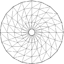
(a) $r=1,\theta=0^{o}$

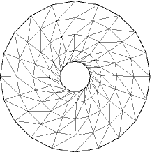
(b) $r=2,\theta=20^{o}$

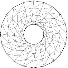
(c) $r=3,\theta=40^{o}$

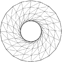
(d) $r=3.5,\theta=50^{o}$

Recall that $\Omega$ is the original polygonal or polyhedral domain, and that $\hat{\Omega}$ is the domain whose boundary is given by the user-specified deformation of the boundary vertices of $\Omega$, i.e., by the vertices at coordinates $(\hat{x}_{B},\hat{y}_{B})$. Assume that this user-specified deformation is not self-intersecting and preserves orientation.

Let $\phi$ be the mapping from $\Omega$ to $\hat{\Omega}$ computed by FEMWARP. In other words, interpolate the interior vertex deformations linearly over the elements to arrive at a continuous function on the whole domain. (In the case that FEMWARP fails, parts of $\phi(\Omega)$ may protrude outside of $\hat{\Omega}$.)

Let $\phi^{*}$ be the mapping that is obtained from the exact (continuum) Laplacian. In other words, solve the boundary value problems

$$\bigtriangleup\hat{x} = 0\quad\mbox{on $\Omega$},$$

$$\bigtriangleup\hat{y} = 0\quad\mbox{on $\Omega$},$$

$$\hat{x} = \hat{x}_{B}\quad\mbox{on $\partial\Omega$},$$

$$\hat{y} = \hat{y}_{B}\quad\mbox{on $\partial\Omega$}$$

and define $\phi^{*}(x,y)=(\hat{x}(x,y),\hat{y}(x,y))$. Let us call this warping algorithm “continuum FEMWARP”.

Finally, let $\phi^{+}$ be the mapping that is obtained by linear interpolation over the elements of $\phi^{*}$ evaluated at vertices. Thus, $\phi^{+}$ is intermediate between $\phi$ and $\phi^{*}$ in the sense that for $\phi^{+}$ we use the exact solution to the continuum problem only at vertex points and use interpolation elsewhere.

There are three possible reasons that FEMWARP could fail:

1. Mapping $\phi^{*}$ might have reversals.

2. Mapping $\phi^{+}$ might have reversals even though $\phi^{*}$ has none.

3. Mapping $\phi$ might have reversals even though $\phi^{+}$ has none.

Let us call these Type 1, Type 2, and Type 3 failures. For Type 1 failure, “reversal” means the existence of a point $x\in\Omega$ such that $\nabla\phi(x)$ has a nonpositive determinant. For the second and third types, “reversal” means that a triangle is reversed. Type 1 reversals are caused by the boundary deformation alone and are not related to the mesh. Type 2 reversals are due to continuous versus discrete representation of $\phi^{*}$, and Type 3 reversals can be analyzed using traditional error estimates for the finite element method.

Let us start with Type 1 reversals. It is difficult to characterize inputs for which $\phi^{*}$ will have reversals. In ShontzThesis , a sufficient condition is given for two-dimensional domains to ensure that $\phi^{*}$ will be an invertible function, but the condition is unrealistically stringent and is nontrivial to check in practice.

Rather than presenting the theorem from ShontzThesis , we choose to present a series of examples and discussion on how to avoid reversals. The geometry for most of the examples in this section is a two-dimensional annulus with outer radius 1 and inner radius $r<1$. Meshes used for tests in this section were generated by Triangle, a two-dimensional quality mesh generation package shew . A typical mesh that occurs in some of the experiments is depicted in Fig. 2; this mesh has $1238$ elements, $694$ vertices, and a maximum side length of $0.1137$. Its inner radius is $0.5$.

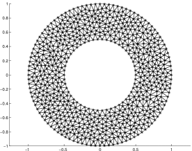
Figure 2: All meshes in this section were generated by the Triangle mesh generator; this is an example of a mesh used herein.

The boundary transformations applied in this section usually consist of two motions: First, the inner circular boundary is moved radially outward (“compression”) to new radius $s$ such that $r\leq s<1$. Second, a rotation of magnitude $\theta$ is applied to the outer boundary. The relevant Laplace equations determining $\phi^{*}$ can be solved in closed form to yield

$$\phi^{*}(x,y)=(Ax+By,-Bx+Ay)$$

where $A=a+b/(x^{2}+y^{2})$ and $B=c+d/(x^{2}+y^{2})$, and $a,b,c,d$ are constants determined by the boundary conditions. In particular, to match the boundary conditions just described, one must satisfy the equations $a+b=\cos\theta$, $c+d=\sin\theta$, $a+b/r^{2}=s/r$, $c+d/r^{2}=0$. These equations are uniquely solved by choosing

$$\{a,b,c,d\}=\frac{\{\cos(\theta)-rs,rs-r^{2}\cos(\theta),\sin(\theta),-r^{2}\sin(\theta)\}}{1-r^{2}}.$$ (7)

This function $\phi^{*}$ is invertible, i.e., avoid reversals, provided the determinant of its Jacobian is always positive. This determinant may be computed in closed form: $\det(\nabla\phi^{*})=a^{2}+c^{2}-(b^{2}+d^{2})/(x^{2}+y^{2})^{2}$. This quantity is minimized when $x^{2}+y^{2}=r^{2}$. Therefore, reversals of Type 1 occur if and only if $r^{2}(a^{2}+c^{2})\leq b^{2}+d^{2}$. Substituting the above formulas for $a,b,c,d$ yields the result that reversals occur if and only if

$$2r\cos(\theta)-r^{2}s-s<0.$$

For example, if $r=s=0.5$ (no compression), then reversals occur when $\cos(\theta)<.625$, i.e., $\theta\geq 51.4...^{\circ}$. If $r=.5$ while $s=.75$, then reversals occur when $\theta\geq 20.4...^{\circ}$.

We tested the FEMWARP algorithm on the cases described above with a mesh for the annular region as discussed earlier. We used a mesh with inner radius $r=0.5$. This particular mesh contained 10,950 triangles with maximum side length of 0.039. For $s=0.5$, when we selected $\theta=51^{\circ}$, FEMWARP ran on this mesh without reversals, whereas $\theta=52^{\circ}$ caused reversals. As mentioned in the previous paragraph, $\theta\approx 51.4^{\circ}$ is the cutoff for Type 1 reversals. When $r=0.5$, $s=0.75$, FEMWARP succeeded for $\theta=22^{\circ}$ but failed for $\theta=23^{\circ}$, again, very close to the cutoff for Type 1 reversals.

In addition, we tested the FEMWARP algorithm on two meshes on a cylinder geometry with height 2 and radius $r=1$. The first mesh was a coarse mesh containing 4320 unstructured tetrahedra which were arranged in 10 layers with 432 tetrahedra per layer. The second mesh was a fine mesh containing 101,550 tetrahedra which were arranged in 25 layers with 4062 tetrahedra per layer. Each cylinder mesh was created by first using Triangle to generate a mesh on a disk and second using our own software to extrude the tetrahedral mesh in layers. The boundary deformation used for the experiment was $(r\cos(\theta),r\sin(\theta),z)\mapsto(r\cos(\theta+tz),r\sin(\theta+tz),z),$ where $t$ is a parameter which controls the amount of deformation. When $t=0$, no deformation occurs, whereas increasing values of $t$ correspond to increasing amounts of deformation. In each case, the value of $t$ was increased in increments of $0.1$, thus applying an increasing amount of deformation to the boundary, until element reversal occurred. On the coarse mesh, FEMWARP succeeded for $t^{\rm max}_{\rm coarse}=5.1$ and failed for $t^{\rm fail}_{\rm coarse}=5.2$, whereas on the fine mesh, it succeeded for $t^{\rm max}_{\rm fine}=5$ and failed for $t^{\rm fail}_{\rm fine}=5.1$. The element reversal which occurs on the fine mesh for $t^{\rm max}_{\rm fine}=5$ is considered a Type 1 reversal because the fine mesh is very close to the true Laplace solution, and a Type 1 reversal means that the true Laplace solution has a Jacobian with a nonpositive determinant. On the other hand, when a reversal occurs on the coarse mesh, it could be either Type 1, Type 2, or Type 3. Because $t^{\rm max}_{\rm coarse}$ is close to $t^{\rm max}_{\rm fine}$, it is safe to conclude that the reversals in the coarse mesh are usually Type 1.

The point of the experiments in the previous two paragraphs is that for a reasonably refined and reasonably high-quality mesh, most FEMWARP reversals seem to be Type 1 reversals. In other words, FEMWARP fails when continuum FEMWARP fails or is close to failure. Other experiments not reported here seem to confirm this point. Therefore, in order to extend the range of deformations that can be handled by FEMWARP, the best strategy is to come up with a way to avoid Type 1 reversals.

One simple method to avoid Type 1 reversals is to take several smaller steps instead of one big step. For example, suppose $(\hat{x}_{B}^{\prime},\hat{y}_{B}^{\prime})$ are positions for the boundary vertices intermediate between their initial positions and their final positions $(\hat{x}_{B},\hat{y}_{B})$. Then one could define a two-step continuum FEMWARP as follows. Solve

$$\bigtriangleup\hat{x}^{\prime} = 0\quad\mbox{on $\Omega$},$$

$$\bigtriangleup\hat{y}^{\prime} = 0\quad\mbox{on $\Omega$},$$

$$\hat{x}^{\prime} = \hat{x}_{B}^{\prime}\quad\mbox{on $\partial\Omega$},$$

$$\hat{y}^{\prime} = \hat{y}_{B}^{\prime}\quad\mbox{on $\partial\Omega$}$$

for $\hat{x}^{\prime}$ and $\hat{y}^{\prime}$ to determine a mapping $\phi_{1}:\Omega\rightarrow\Omega^{\prime}$ given by $(x,y)\mapsto(\hat{x}^{\prime},\hat{y}^{\prime})$ (where $\Omega^{\prime}$ is the domain bounded by $(\hat{x}_{B}^{\prime},\hat{y}_{B}^{\prime})$) followed by

$$\bigtriangleup\hat{x} = 0\quad\mbox{on $\Omega^{\prime}$},$$

$$\bigtriangleup\hat{y} = 0\quad\mbox{on $\Omega^{\prime}$},$$

$$\hat{x} = \hat{x}_{B}\quad\mbox{on $\partial\Omega^{\prime}$},$$

$$\hat{y} = \hat{y}_{B}\quad\mbox{on $\partial\Omega^{\prime}$}$$

for $\hat{x}$, $\hat{y}$ to obtain a map $\phi_{2}$. Finally, $\phi^{*}=\phi_{2}\circ\phi_{1}$.

The idea in the previous paragraph can be extended to more steps with smaller increments. The limiting case of an infinite number of infinitesimal steps yields an algorithm that we call “infinitesimal-step continuum FEMWARP.” Infinitesimal-step FEMWARP can be described formally as follows. Let the initial domain be denoted as $\Omega\subset{\bf R}^{d}$ with boundary $\Gamma$. Assume there is a $C^{1}$ function $g:\Gamma\times{\bf R}\rightarrow{\bf R}^{d}$ such that $g(x,0)\equiv x$; this function $g$ describes the motion of the boundary. Here $d=2$ or $d=3$. Thus, the boundary at time $t$ is denoted as $\Gamma(t)$ and satisfies $\Gamma(t)=g(\Gamma,t)$. It is assumed that $g(x,t)$ is injective as a function of $x$, so that the boundary never intersects itself.

The step at time $t$ is determined by the derivative of $g$. In particular, let us define a function $G(x,t)$, where $x\in\Omega(t)$, as follows. Temporarily fix a particular $t$. Solve the vector-valued Laplace equation for $u:\Omega(t)\rightarrow{\bf R}^{d}$ (i.e., a separate Laplace equation for each coordinate entry) given by

$$\begin{array}[]{rcll}\bigtriangleup u(x)&=&0&\mbox{for $x\in\Omega(t)$,}\\ u(x)&=&\frac{\partial}{\partial t}g(g^{-1}(x,t),t)&\mbox{for $x\in\Gamma(t)$}.\end{array}$$

Finally, define $G(x,t)=u(x)$. Last, given a point $x_{0}\in\Omega$, we consider the trajectory defined by the initial value problem $x(t)=x_{0}$; $x^{\prime}(t)=G(x,t)$. The solution operator of this ODE system, say $\Phi(x,t)$, defines the infinitesimal-step continuum FEMWARP mapping at time $t$.

It can be shown that this map is a bijection with a positive Jacobian for all $x$ (i.e., no reversals). This is a consequence of the well-known standard fact that the solution operator for an ODE system with a Lipschitz forcing function $G$ is bijective with a positive Jacobian. The usual textbook theorem does not quite apply to this case because the spatial domain of $G(x,t)$ is not fixed in time but depends on $t$. However, the theorem is still valid because for any $x_{0}$ interior to $\Omega(t)$, one can break up the trajectory into small pieces and define $G(x,t)$ only in a small neighborhood around $x$ (but fixed over time for each piece). Then the pieces can be assembled together to prove the result.

In the case of the annulus, it is possible again to write down infinitesimal-step continuum FEMWARP in closed form. For simplicity, let us assume $r=s$ so that the only deformation is the rotation of the outer boundary. Assume this rotation is broken up into infinitesimally small rotations. (Another choice would be to connect the initial positions to the final positions with line segments, and break up the boundary motion as infinitesimal increments along the line segments. This way to obtain a continuous boundary motion is undesirable, however, because for a sufficiently large rotation, the line segments would cut through the inner boundary of the annulus and hence cause tangling of the boundaries.)

With the setup described in the last paragraph, the deformation for an outer rotation of $\theta$ computed by infinitesimal-step continuum FEMWARP maps a point at initial position $\rho(\cos\phi,\sin\phi)$ ($r\leq\rho\leq 1$) to $\rho(\cos(\phi+\alpha),\sin(\phi+\alpha))$, where $\alpha=(1-r^{2}/\rho^{2})\theta/(1-r^{2})$. This map is clearly bijective for any value of $\theta$; it corresponds to rotating each concentric circle of the annulus by an amount that interpolates between 0 (when $\rho=r$) and $\theta$ (when $\rho=1$).

Thus, by using small-step FEMWARP with sufficiently small steps, we can essentially eliminate Type 1 failures. Small-step FEMWARP preserves the attractive property of FEMWARP that it is exact for affine maps, as long as all the intermediate steps are also affine. Unfortunately, it loses the attractive property that only one coefficient matrix for solving the linear system needs to be factored. Small-step FEMWARP requires the solution of a different coefficient matrix for each step. This drawback is partly ameliorated by the fact that even though the matrices are different, they have the same nonzero pattern, and hence the symbolic phase of sparse direct solution may be reused. If instead an iterative method is being used to solve the mesh warping equations, then the sparsity pattern may be reused in the preconditioner. In addition, the factored coefficient matrix at step $t_{k}$ can be used as a preconditioner for an iterative method at step $t_{k+1}$.

Elimination of Type 1 failures means that the mapping function $\phi^{*}$ has no reversals in the sense that the determinant of its Jacobian is positive everywhere; equivalently, it does not reverse any infinitesimally small triangles. A Type 2 failure occurs because the triangles in the mesh have finite (non-infinitesimal) size and hence can still be reversed by $\phi^{+}$. The following theorem characterizes when this can happen.

Theorem 4.1

Suppose that $f:\Omega\rightarrow{\bf R}^{2}$ is bijective, orientation-preserving and $C^{2}$ on $\Omega$ with $\nabla f$ nonsingular. Let $T$ be a triangle in the mesh with vertices $\{v_{1},v_{2},v_{3}\}$, and let $T^{\prime}$ be the triangle whose vertices are $\{f(v_{1}),f(v_{2}),f(v_{3})\}$. If $(\ref{eq:revineq})$ below holds, then $T^{\prime}$ is not reversed.

Proof

Recall that triangle $T$ with vertices $\{v_{1},v_{2},v_{3}\}$ is positively oriented if and only if $\det(A)>0$, where

$$A=(v_{2}-v_{1},v_{3}-v_{1}).$$

In order to analyze the analogous quantity for $\{f(v_{1}),f(v_{2}),f(v_{3})\}$, we start with the following algebra, which invokes the fundamental theorem of calculus twice:

$$f(v_{2})-f(v_{1}) = \int_{0}^{1}\nabla f((1-t)v_{1}+tv_{2})(v_{2}-v_{1})\,dt$$

$$= \left(\int_{0}^{1}\nabla f((1-t)v_{1}+tv_{2})\,dt\right)(v_{2}-v_{1})$$

$$= \left(\nabla f(v_{1})+\int_{0}^{1}\left[\nabla f((1-t)v_{1}+tv_{2})-\nabla f(v_{1})\right]\,dt\right)(v_{2}-v_{1})$$

$$= \nabla f(v_{1})(v_{2}-v_{1})$$

$$+\left(\int_{0}^{1}\left[\int_{0}^{1}\nabla^{2}tf((1-s)v_{1}+s((1-t)v_{1}+tv_{2}))(v_{2}-v_{1})\,ds\right]\,dt\right)$$

$$\ \ \ \ \ \ \ \ \ \ \ \ \ (v_{2}-v_{1})$$

$$= \nabla f(v_{1})(v_{2}-v_{1})+e_{1}$$

where $\|e_{1}\|\leq Mh^{2}$, where $h$ is the maximum side length of $T$ (an upper bound on $\|v_{2}-v_{1}\|$) and $M$ is an upper bound on $\|\nabla^{2}f\|$ in the triangle. Similarly,

$$f(v_{3})-f(v_{1})=\nabla f(v_{1})(v_{3}-v_{1})+e_{2},$$

where again $\|e_{2}\|\leq Mh^{2}$. Therefore,

$$(f(v_{2})-f(v_{1}),f(v_{3})-f(v_{1}))=\nabla f(v_{1})A+E$$ (8)

where $A$ is as above and $\|E\|_{2}\leq\sqrt{2}Mh^{2}$. Observe that $\nabla f(v_{1})A$ has positive determinant by assumption. Therefore, the left-hand side can have negative determinant only if $E$ is a sufficiently large perturbation to change the determinant sign. If $E$ is such a large perturbation, then by the continuity of the determinant, there is a perturbation $E^{\prime}$ no larger than $E$ such that the $\det(\nabla f(v_{1})A+E^{\prime})=0$, i.e., $\nabla f(v_{1})A+E^{\prime}$ is singular. Furthermore, $\|E^{\prime}\|\leq\sqrt{2}Mh^{2}$. By Theorem 2.5.3 of GVL3 , this means that

$$\sqrt{2}Mh^{2}\geq\sigma_{\min}(\nabla f(v_{1})A)\geq\sigma_{\min}(\nabla f(v_{1}))\sigma_{\min}(A),$$ (9)

where $\sigma_{\min}(A)$ and $\sigma_{\max}(A)$ denote the smallest and largest singular values of $A$, respectively. It follows from the equation $AA^{-1}=I$ that that the columns of $A^{-1}$ are parallel to the altitude segments of triangle $T$ perpendicular to $v_{1}v_{3}$ and $v_{1}v_{2}$ respectively, but scaled so that their lengths are the reciprocals of those altitude lengths. Therefore, $\sigma_{\max}(A^{-1})\leq\sqrt{2}/\mathop{\rm minalt}(T)$, where $\mathop{\rm minalt}(T)$ means the minimum altitude. Thus, $\sigma_{\min}(A)\geq\mathop{\rm minalt}(T)/\sqrt{2}$. Substituting this inequality into $(\ref{eq:Mh2})$ and rearranging yields

$$\frac{\sigma_{\min}(\nabla f(v_{1}))}{M}\leq 2h\mathop{\rm asp}(T)$$

where $\mathop{\rm asp}(T)$, the aspect ratio of $T$, equals $h/\mathop{\rm minalt}(T)$. The aspect ratio is often used as a shape-quality metric; lower values mean a better shaped triangle. Thus, reversal cannot happen if the opposite inequality holds:

$$\frac{\sigma_{\min}(\nabla f(v_{1}))}{M}>2h\mathop{\rm asp}(T).$$ (10)

The point of this theorem is that Type 2 reversals cannot occur for a sufficiently refined mesh (i.e., $h$ sufficiently small in $(\ref{eq:revineq})$), assuming that the mesh quality does not decay, and assuming that $\phi^{*}$ is a nonsingular function. (Assuming Type 1 reversals are excluded, function $\phi^{*}$ is never singular on the interior because Laplace solutions are analytic. It could be singular at the boundary if, for example, $\Omega^{\prime}$ has a corner where $\Omega$ had none.)

We tested this theorem for two examples, each of which diverges a bit from the theoretical prediction. For the first example, we generated a uniform mesh for the rectangle $[0,2]\times[0,1]$ using Triangle and mapped all the vertices using the function $f(x,y)=(x,y+\alpha x(2-x))$. For each mesh, $\alpha$ was incremented by 1 until reversal occurred. (No Laplace solution was involved in this test case.) We tabulated the values of $h$ versus $\alpha$ in Table 1. As predicted by the theorem, the table shows that as $h$ decreases, a larger value of $\alpha$ is tolerated. Contrary to the theorem, however, the table shows that $\sigma_{\min}(\nabla f)/\|\nabla^{2}f\|$ is decreasing faster than $h$. In other words, reversals are avoided to a greater extent than predicted by the theorem. The reason for this discrepancy is that the perturbation term $E$ in $(\ref{eq:pertAE})$ is not well aligned with the direction that drives $(\nabla f)A$ toward singularity in this example. In particular, $E$ affects only the $y$-components (since the transformation is linear for $x$-coordinates). On the other hand, transformation $\phi$ stretches the triangles substantially in the $y$-direction, so that the most effective way to perturb $(\nabla f)A$ toward singularity is a small change to the $x$-components.

As a second test case, consider the transformation of the annulus with radii $(0.5,1)$ that results from continuous-warping continuum FEMWARP, that is, the transformation that rotates a point at radius $\rho$ by angle $\alpha(1-r^{2}/\rho^{2})/(1-r^{2})$, where $r$ is the inner radius ($r=0.5$ for this test). For each mesh, the parameter $\alpha$ was stepped in increments of $\pi/16$ until reversals were encountered. We tabulated values of $h$ versus the first of $\alpha$ causing failure in Table 2. As predicted by the theorem, decreasing $h$ corresponded to increasing values of $\alpha$, i.e., greater distortion of the domain. Again, these results do not initially correspond to the preceding theorem quantitatively: in this case, $h$ is decreasing faster than $\sigma_{\min}(\nabla f)/\|\nabla^{2}f\|$. Only the last three rows of the table show that $h$ and $\sigma_{\min}(\nabla f)/\|\nabla^{2}f\|$ are decreasing proportionally. The reason for this discrepancy is that $\nabla^{2}f$ is much larger on the inner boundary than elsewhere, and the meshes in the initial rows of the table are not sufficiently refined to resolve the variation in the value of the derivative.

Table 1: Second column $\alpha^{\rm fail}$ is the first value of $\alpha$ in the transformation $(x,y)\mapsto(x,y+\alpha x(2-x))$ of a rectangle that causes reversals in the mesh. The first column shows the mesh cell size (maximum edge length). The third column is $\sigma_{\min}(\nabla f)/\|\nabla^{2}f\|$ evaluated at a vertex of a triangle that reversed.

$h$	$\alpha^{\rm fail}$	$\sigma_{\min}(\nabla f)/\|\nabla^{2}f\|$
0.205	10	$4.6\cdot 10^{-3}$
0.108	14	$2.5\cdot 10^{-3}$
0.057	30	$5.7\cdot 10^{-4}$
0.030	51	$1.9\cdot 10^{-4}$
0.015	95	$5.6\cdot 10^{-5}$

Table 2: Second column $\alpha^{\rm fail}$ is the first value of $\alpha$ in the transformation $(\rho,\theta)\mapsto(\rho,\theta+\alpha(1-r^{2}/\rho^{2})/(1-r^{2}))$ (in polar coordinates) of an annulus that causes reversals in the mesh. The first column shows the mesh cell size (maximum edge length). The third column is $\sigma_{\min}(\nabla f)/\|\nabla^{2}f\|$ evaluated at a vertex of a triangle that reversed.

$h$	$\alpha^{\rm fail}$	$\sigma_{\min}(\nabla f)/\|\nabla^{2}f\|$
0.202	$7\pi/16$	$6.9\cdot 10^{-3}$
0.114	$\pi/2$	$4.6\cdot 10^{-3}$
0.058	$9\pi/16$	$6.2\cdot 10^{-3}$
0.031	$5\pi/8$	$2.5\cdot 10^{-3}$
0.015	$11\pi/16$	$2.6\cdot 10^{-3}$
0.008	$13\pi/16$	$1.4\cdot 10^{-3}$
0.004	$\pi$	$7.2\cdot 10^{-4}$

Thus, we have seen that Type 1 reversals can be avoided by using small-step FEMWARP instead of FEMWARP, and Type 2 reversals can be avoided by using a sufficiently refined mesh. The remaining type of reversals, Type 3, are rare according to our experiments. Type 3 reversals are caused by the difference between the true value of the Laplace solution and the finite element approximation to that solution. Intuitively, this phenomenon should not be commonplace because the perturbation size to a mesh necessary to cause a reversal of a triangle of side-length $h$ is $O(h)$, whereas the difference between the two mappings is $O(h^{2})$.

Consider the following test. We generated a sequence of small-step rotations for the annulus in two ways. In the first case, we took steps that rotate the outer boundary by $\pi/16$ and leave the inner boundary invariant, each time computing the Laplace solution exactly analytically. This corresponds to iteratively applying the transformation $\phi^{*}(x,y)=(Ax+By,-Bx+Ay)$ to the mesh, where $A,B,C,D$ are functions of $x^{2}+y^{2}$ as above, and $a,b,c,d$ are constants determined by $(\ref{eq:abcd})$ with $r=s=0.5$, $\theta=\pi/16$. In the second case, we solved Laplace’s equation for the above boundary condition using the finite element mesh that results from small-step FEMWARP. In both cases we tried meshes with several different values of $h$. The results are tabulated in Table 3. As can be seen, discretized small-step FEMWARP outperformed continuum small-step FEMWARP.

In other words, not only did Type 3 reversals not occur, but in fact it seems to be preferable to use the discretized solution for mesh warping rather than the continuum solution. The difference between $\phi^{+}$ and $\phi$ is the usual discretization error in finite element methods. A possible explanation for the improved resistance to reversals of the finite element solution is as follows. After several steps of small-step FEMWARP, Laplace’s equation is solved on a mesh with mostly poorly-shaped elements, some extremely poorly-shaped. A Laplace solution minimizes the functional $F(u)=\int_{\Omega}\nabla u\cdot\nabla u$ over $H^{1}$ functions $u$ on the domain, and the finite element solution minimizes the same functional $F(u)$ over the space of piecewise linear choices for $u$ johnsonbook . A very poorly-shaped element is “stiffer” than others in the following sense. An affine linear function $u$ defined over a triangle that has an angle close to $180^{\circ}$ will have a quite large gradient value (compared to a well-shaped triangle with the equal area and equal vertex values) unless the vertex values lie in a certain restricted range. Therefore, the extra stiffness of these elements will cause them to be deformed less than the better-shaped elements in the optimal solution that minimizes $F$. Since the poorly-shaped elements are those most in danger of being reversed, this is a desirable effect.

Table 3: Continuum versus discretized small-step FEMWARP applied to a mesh of an annulus in order to test for Type 3 reversals. The table shows that discretized small-step FEMWARP seems less prone to reversals than continuum small-step FEMWARP.

$h$	$\alpha^{\rm fail}_{\rm continuum}$	$\alpha^{\rm fail}_{\rm discrete}$
$0.202$	$7\pi/16$	$\pi/2$
$0.114$	$\pi/2$	$9\pi/16$
$0.058$	$9\pi/16$	$5\pi/8$
$0.031$	$5\pi/8$	$7\pi/8$
$0.015$	$11\pi/16$	$\pi$

The next topic to consider in this section is how to select a stepsize for small-step FEMWARP. The theory developed above indicates that as long as the step size is well below a step large enough to cause reversals of $\phi^{*}$, the step size should not matter so much. In fact, we propose the following simple strategy, which seems to be effective. Attempt to take a very large step (e.g., a rotation of size $\pi$ in the case of the annulus). If this fails (causes reversals), then halve the stepsize and try again until success. Update the mesh and try another such step. Note that in the process of searching for a correct stepsize, the coefficient matrix in FEMWARP is the same for each trial. Therefore, the Cholesky factors do not need to be recomputed until the mesh is updated.

Another way to carry out small-step FEMWARP would be to take constant (small) steps on each iteration. We compared these two methods and found that the first was much more efficient, and furthermore, reversals are resisted better by the first strategy. Therefore, the repeated halving strategy is recommended. Table 4 summarizes the result for the annulus again. For the halving strategy, updates were pursued until the stepsize dropped below $\pi/128$. For the constant-step strategy, the stepsize was taken to be $\pi/128$.

Table 4: Variable stepsize versus constant stepsize for small-step FEMWARP applied to a mesh of an annulus. Second and third columns are the maximum amount of rotation prior to reversals for the two methods. Fourth and fifth columns are the number of Cholesky factorizations required by the two methods.

$h$	$\alpha^{\rm max}_{\rm VS}$	$\alpha^{\rm max}_{\rm CS}$	$\mbox{NCHOL}_{\rm VS}$	$\mbox{NCHOL}_{\rm CS}$
$0.202$	$1.7426$	$1.7671$	$13$	$72$
$0.114$	$2.2089$	$2.0862$	$24$	$85$
$0.058$	$2.6998$	$2.4789$	$29$	$101$
$0.031$	$3.4852$	$2.7980$	$34$	$114$

The final workaround to element reversal we consider in this section is to use, instead of the discrete harmonic map, the mean value map floater2 for computing the weights. The mean value map satisfies the same affine exactness as the discrete harmonic map (as shown in Lemma 3.1), and because of this may tend to give similar results to the discrete harmonic map. Yet, at the same time, the mean value map uses weights that are always nonnegative (regardless of the shapes of the triangles), and so at least for a convex boundary, it guarantees an injective map floater2 .

In order to compare the performance of FEMWARP to that of the algorithm using the mean value map, two experiments were performed. The first experiment was on an annulus mesh with radii $(0.5,1)$ which was composed of 10840 triangles. A rotation of magnitude $\theta$ was applied to the outer boundary. For both algorithms, $\theta=50^{o}$ was the maximum amount of deformation which could be successfully applied; a deformation with $\theta=51^{o}$ yielded element reversal. Thus, the two algorithms did not realize a difference in performance for this experiment.

The second experiment was on an annulus mesh with radii (0.3,1) which was composed of 13162 triangles. For this experiment, the boundary deformation that rotates a point at radius $\rho$ by angle $\alpha(\rho-r)/(1-r)$, where $r$ is the inner radius ($r=0.3$ for this test). This corresponds to rotating each concentric circle of the annulus by an amount that interpolates between 0 (when $\rho=r$) and $\alpha$ (when $\rho=1$). The parameter $\alpha$ was stepped in increments of $0.05$ until reversals were encountered. In this case, FEMWARP was able to perform 52 rotation steps successfully, whereas the mean value map algorithm only performed 24 steps before element reversal occurred. Thus, the discrete harmonic map used in FEMWARP generates weights which allow for successful application of larger deformations than those tolerated by the mean value map.

5 Mesh warping and mesh untangling

In the previous section we considered reasons why FEMWARP can fail and also some possible workarounds. Some of the workarounds in the previous section, however, are not available in all circumstances. For example, the workaround for Type 1 reversals, namely, small-step FEMWARP, requires a homotopy from the old to new boundary conditions and also requires solution of many linear systems with distinct coefficient matrices. Although linear interpolation could be performed if a homotopy from the old to new boundary conditions is not available, FEMWARP probably would not give the desired motion, e.g., if the boundary deformation involves some kind of rotation. The workaround for Type 2 reversals requires refined meshes, which may not be available.

Another workaround is to switch to a different algorithm, for example, Opt-MS, a mesh untangling method due to Freitag and Plassmann FreitagPlassmann . Opt-MS takes as input an arbitrary tangled mesh and a specification of which vertices are fixed (i.e., boundary vertices) and which are movable. It then attempts to untangle the mesh with a sequence of individual vertex moves based on linear programming. More details are provided below.

In this section, we consider the use of Opt-MS for mesh warping. We find that the best method is a hybrid of FEMWARP and Opt-MS.

To untangle the mesh, Opt-MS performs repeated sweeps over the interior vertices. For each interior vertex, it repositions the vertex at the coordinates that maximize the minimum signed area (volume) of the elements adjacent to that vertex (called the “local submesh”). The signed area is negative for a reversed element, so maximizing its minimum value is an attempt to fix all reversed elements.

Let ${\bf x}$ be the location of the free vertex, that is, the current interior vertex being processed in a sweep. Let ${\bf x}_{1},\ldots,{\bf x}_{p}$ be the positions of its adjacent vertices, and $t_{1},\ldots,t_{n}$ be the incident triangles (tetrahedra) that compose the local submesh. Then the function that prescribes the minimum area (volume) of an element in the local submesh is given by $q({\bf x})=\min_{1\leq i\leq n}\ A_{i}({\bf x})$, where $A_{i}$ is the area (volume) of simplex $t_{i}$. In 2D, the area of triangle $t_{i}$ can be stated as a function of the Jacobian of the element as follows: $A_{i}=\frac{1}{2}\det({\bf x}_{i}-{\bf x},\ {\bf x}_{j}-{\bf x})$ which is a linear function of the free vertex position; the same is true in 3D. Freitag and Plassmann use this fact to formulate the solution to $\max q({\bf x})=\max\min_{1\leq i\leq n}\ A_{i}({\bf x})$ as a linear programming problem which they solve via the simplex method. On each sweep, $m$ linear programs are solved which sequentially reposition each interior vertex in the mesh. Sweeps are performed until the mesh is untangled or a maximum number of sweeps has occurred.

A shortcoming of Opt-MS, in comparison to FEMWARP, is that it is not intended to handle a very large boundary motion even if that motion is affine. For example, starting from a 2D mesh, if the boundary vertices are all mapped according to the function $(x,y)\mapsto(-x,-y)$ while the interior vertices are left unmoved, in many cases Opt-MS is unable to converge. FEMWARP, on the other hand, will clearly succeed according to Theorem 1.

Therefore, we propose the following algorithm: one applies first the FEMWARP mesh warping algorithm, and if the mesh is tangled, one uses Opt-MS to untangle the mesh output by FEMWARP (as opposed to the original mesh). The rationale for this algorithm is that FEMWARP is better able to handle the gross motions while Opt-MS handles the detailed motion better.

To test whether this algorithm works, we applied it again to the mesh depicted in Fig. 2. The boundary motion is as follows: we rotate the outer circular boundary by $\theta_{1}$ degrees and the inner boundary by $\theta_{2}$ degrees and then test three algorithms: FEMWARP alone, Opt-MS alone, and hybrid. (The hybrid was tested only in the case that the two algorithm individually both failed.) The results are tabulated in Table 5. The table makes it clear that the hybrid often works when Opt-MS and FEMWARP both fail. Thus, the hybrid method is another technique for situations when FEMWARP alone fails and small-step FEMWARP combined with mesh refinement may be unavailable. The hybrid method has the disadvantage, when compared to FEMWARP, that it does not produce a continuous motion of interior vertices but rather only a final configuration.

Table 5: The row header indicates $\theta_{1}$ (degrees), the rotation of the outer boundary, and the column header $\theta_{2}$ is the rotation of the inner boundary. The table entries are as follows: ‘F’ means FEMWARP succeeded but not Opt-MS, ‘O’ means Opt-MS succeed but not FEMWARP,‘B’ means both succeeded, and ‘H’ means neither succeeded, but the hybrid succeeded, and finally ‘–’ means none succeeded.

$\theta_{1}\backslash\theta_{2}$	$0$	$15$	$30$	$45$	$60$	$75$	$90$	$105$	$120$	$135$	$150$	$165$	$180$
$0$	B	B	B	B	O	O	O	–	–	–	–	–	–
$15$	B	B	B	B	B	O	O	H	–	–	–	–	–
$30$	B	B	B	B	B	B	H	O	H	–	–	–	–
$45$	B	B	B	B	B	B	B	O	O	H	–	–	–
$60$	O	B	B	B	B	B	B	B	O	O	H	–	–
$75$	O	O	B	B	B	B	B	B	B	H	H	H	–
$90$	O	O	O	B	B	B	B	B	B	B	O	H	H
$105$	O	O	O	O	B	B	B	B	B	F	B	O	H
$120$	–	–	H	H	H	B	B	B	F	F	B	F	H
$135$	–	–	–	H	H	H	F	B	B	B	B	B	B
$150$	–	–	–	–	H	H	H	F	B	B	B	B	B
$165$	–	–	–	–	–	H	H	H	F	F	B	B	B
$180$	–	–	–	–	–	–	H	H	H	F	B	B	B

6 Three-dimensional tests

In this section we compare the robustness against reversals of FEMWARP, small-step FEMWARP, and the hybrid FEMWARP/Opt-MS method on examples of 3D meshes pat_mesh and lori_mesh shown in Figure 3.

Figure 3: The 3D test meshes used in this section: (a) foam5 pat_mesh , (b) gear pat_mesh , (c) hook pat_mesh , and (d) tire lori_mesh .

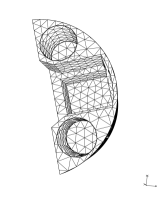
(a) foam5

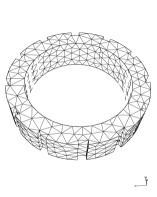
(b) gear

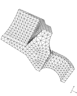
(c) hook

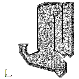
(d) tire

We choose specific nonlinear boundary deformations parameterized by a scalar $\alpha$ in order to determine how much deformation each test mesh could withstand when warped according to each method:

$$\left(\begin{array}[]{c}x\\ y\\ z\end{array}\right)\mapsto\left(\begin{array}[]{rrr}2&-1&0\\ -2&5&0\\ 0&0&1\\ \end{array}\right)\left(\begin{array}[]{c}x\\ y\\ z\end{array}\right)+\alpha\left(\begin{array}[]{c}0.1xy\\ 0.5yz\\ 0.1x^{2}\end{array}\right).$$

Table 6 gives the results obtained from warping various three-dimensional meshes according to this boundary deformation. The data in this table is as follows. The first three columns give the name of the mesh, the number of boundary vertices, and the number of total vertices. The fourth column $\alpha_{\rm FEMWARP}^{\rm max}$ gives the maximum value of $\alpha$ encountered for which FEMWARP succeeded. Parameter $\alpha$ was stepped by $\Delta\alpha$, where $\Delta\alpha$ is indicated in the last column of the table. Table 7 is a continuation of the previous table. The second and third columns of this table show $\alpha_{\rm ssFEMWARP}^{\rm max}$, which is the last value of $\alpha$ for which small-step FEMWARP succeeds, and $\mbox{NCHOL}_{\rm SS}$, which is the number of Cholesky factorizations required by small-step FEMWARP. The variable-step version of FEMWARP described in Section 4 was used. The minimum allowed stepsize for small-step FEMWARP was also taken to be $\Delta\alpha$.

The table indicates that small-step FEMWARP was about equal in robustness against reversals compared with FEMWARP except for the last mesh. In the case of “tire”, small-step FEMWARP was much more robust. This is probably because the reversals in the first three rows are primarily Type 2 reversals since the meshes are very coarse, whereas the “tire” mesh is finer and is therefore more likely to see Type 1 reversals according to the arguments given in the previous section. Small-step FEMWARP is intended to fix Type 1 reversals but is not effective against Type 2 reversals.

We also compared Opt-MS and the hybrid FEMWARP/Opt-MS method described in the last section. These results are shown in the fourth and fifth columns of Table 7. The minimum allowed stepsize for the algorithms was again taken to be $\Delta\alpha$ as shown in the last column of the table. Opt-MS performed poorly because, as mentioned earlier, it is not designed to handle large boundary motions. The performance of the hybrid is comparable, and in some cases superior, to that of small-step FEMWARP.

Table 6: Values of $\alpha^{\rm max}$ for FEMWARP on example three-dimensional meshes.

Mesh name	# bdry vertices	# vertices	$\alpha^{\rm max}_{\rm FEMWARP}$	$\Delta\alpha$
foam5	1048	1337	$0.7$	$0.1$
gear	606	866	$3.5$	$0.1$
hook	790	1190	$0.16$	$0.01$
tire	1248	2570	$0.15$	$0.05$

Table 7: Values of $\alpha^{\rm max}$ for FEMWARP derivative algorithms on example three-dimensional meshes.

Mesh name	$\alpha^{\rm max}_{\rm ssFEMWARP}$	$\mbox{NCHOL}_{\rm SS}$	$\alpha^{\rm max}_{\rm Opt-MS}$	$\alpha^{\rm max}_{\rm hybrid}$	$\Delta\alpha$
foam5	$1.0$	$4$	$0$	$1.2$	$0.1$
gear	$3.5$	$4$	$0.6$	$3.5$	$0.1$
hook	$0.16$	$2$	$0$	$0.16$	$0.01$
tire	$1.60$	$13$	$0$	$2.0$	$0.05$

7 Conclusions

We studied an algorithm called FEMWARP for warping triangular and tetrahedral meshes. The first step in the algorithm is to determine a set of local weights for each interior vertex using finite element methods. Second, a user-supplied deformation is applied to the boundary vertices. The third and final step is to solve a system of linear equations based upon the weights and the new positions of the boundary vertices to determine the final positions of the interior vertices.

There are three main advantages of the FEMWARP algorithm as compared to other mesh-updating methods. First, if a continuous boundary deformation is given, then FEMWARP is valid for computing the resulting trajectory specifying the movement of the interior vertices. In addition, these trajectories will be continuous, which is vital for applications where continuity of motion is required. Second, sparse matrix algorithms may be used to solve the linear system which determines the final positions of the interior vertices. Third, FEMWARP is exact if the boundary deformation is affine.

The main limitation of FEMWARP (as well as most other mesh-updating methods) is that it can fail to yield valid deformed meshes, i.e., it sometimes produces element reversals. Element reversal was our main focus of the paper. We analyzed the case when FEMWARP produced element reversals and proposed four workarounds which include: taking smaller steps, using a finer mesh, employing the mean value map to compute the weights, and, finally, using a hybrid algorithm which combines FEMWARP and Opt-MS.

We tested the robustness of FEMWARP, small-step FEMWARP, a version of FEMWARP which employed the mean value map to compute the weights, and hybrid FEMWARP/Opt-MS on 2D annulus test cases and 3D general unstructured meshes. The use of the mean value map to compute the weights did not improve the performance of FEMWARP on 2D meshes, and hence was not further considered. Small-step FEMWARP and hybrid FEMWARP/Opt-MS generally outperform plain FEMWARP, sometimes significantly. However, an important limitation of the hybrid FEM-WARP/Opt-MS algorithm is that there is no guarantee that Opt-MS eliminates all element reversals. In addition, the algorithm may not preserve the continuous trajectories needed by some applications.

Another limitation of the proposed techniques is that they do not guarantee the quality of the warped mesh. Future work should focus on the development of mesh warping techniques with quality guarantees for the resulting mesh. For example, it may be possible to use optimization in conjunction with the proposed mesh warping techniques in order to develop such quality guarantees. Of course, the resulting algorithms will be likely be more expensive than the current techniques.

In order to reduce the time needed to compute the mesh warping, future work will also focus on the development of an algorithm which formulates a symmetric linear system (instead of forming the symmetric positive definite linear system (2)) expressing the coordinates of each interior vertex in the original mesh in terms of its neighboring vertices. Such a method would belong to the same more general class of methods to which FEMWARP belongs. This more general framework is called the linear weighted Laplacian smoothing framework and was developed by the first author in ShontzThesis . Methods within this framework share many of the same properties as FEMWARP.

The proposed mesh warping techniques in this paper are geometric in nature and do not take into account any knowledge of the particular PDE which may be causing the deformation. Thus, another possibility for future work is to tie the mesh warping techniques to a particular PDE solver so that the deformed mesh is computed as a function of the PDE which is creating the motion in addition to being computed as a function of the particular domain geometry and the deformation upon it. However, the use of such a technique is not always possible. In particular, such a technique could not be used to compute the deformed mesh in conjunction with a discrete set of motion data stemming from a laboratory experiment. The goal of this work was to develop improved mesh warping techniques which more robustly handle deformations in the cases where FEMWARP reverses elements. Some of the proposed techniques are applicable for problems with PDE-based motions, whereas other techniques are applicable for problems with discrete datasets for mesh motions stemming from laboratory experiments.

8 Acknowledgements

The authors wish to thank Dr. Lori Diachin of Lawrence Livermore National Laboratory and Dr. Patrick Knupp of Sandia National Laboratories for providing us with the 3D test meshes. They benefited from conversations with G. Bailey and A. Schatz of Cornell, C. Patron of Risk Capital, T. Tomita of BRM Consulting, and especially H. Kesten, formerly of Cornell. They also wish to thank the two anonymous referees for their careful reading of the paper and for their helpful suggestions which strengthened it.

References

- (1) Antaki, J., Blelloch, G., Ghattas, O., Malcevic, I., Miller, G., Walkington, N.: A parallel dynamic-mesh Lagrangian method for simulation of flows with dynamic interfaces. In: Proceedings of the 2000 Supercomputing Conference, p. 26 (2000)
- (2) Baker, T.J.: Mesh movement and metamorphosis. In: Proceedings of the Tenth International Meshing Roundtable, pp. 387–396. Sandia National Laboratories, Albuquerque, NM (2001)
- (3) Branets, L., Carey, G.: A local cell quality metric and variational grid smoothing algorithm. Eng. Comput. 21, 19–28 (2005)
- (4) Cardoze, D., Cunha, A., Miller, G., Phillips, T., Walkington, N.: A Bézier-based approach to unstructured moving meshes. In: Proceedings of the Twentieth ACM Symposium on Computational Geometry (2004)
- (5) Cardoze, D., Miller, G., Olah, M., Phillips, T.: A Bézier-based moving mesh framework for simulation with elastic membranes. In: Proceedings of the Thirteenth International Meshing Roundtable, pp. 71–80. Sandia National Laboratories (2004)
- (6) Darvish, K., Crandall, J.: Nonlinear viscoelastic effects in oscillatory shear deformation of brain tissue. Med. Eng. Phys. 23, 633–645 (2001)
- (7) Diachin, L.: Personal Communication (October 2002)
- (8) Donders, S., Takahashi, Y., Hadjit, R., Van Langenhove, T., Brughmans, M., Van Genechten, B., Desmet, W.: A reduced beam and joint concept modeling approach to optimize global vehicle body dynamics. Finite Elem. Anal. Des. 45, 439–455 (2009)
- (9) Floater, M.: Mean value coordinates. Comp. Aided Geom. Design 20, 19–27 (2003)
- (10) Floater, M.: One-to-one piecewise linear mappings over triangulations. Math Comp. 72, 685–696 (2003)
- (11) Freitag, L., Plassmann, P.: Local optimization-based simplicial mesh untangling and improvement. Int. J. Numer. Meth. Eng. 49, 109–125 (2000)
- (12) Golub, G.H., Van Loan, C.F.: Matrix Computations, third edn. John Hopkins University Press (1996)
- (13) Helenbrook, B.T.: Mesh deformation using the biharmonic operator. Int. J. Numer. Meth. Eng. 56, 1007–1021 (2003)
- (14) Helm, P., Younes, L., Beg, M., Ennis, D., Leclercq, C., Faris, O., McVeigh, E., Kass, D., Miller, M., Winslow, R.: Evidence of structural remodeling in the dyssynchronous failing heart. Circ. Res. 98, 125–132 (2006)
- (15) Hu, J., Liu, L., Wang, G.: Dual Laplacian morphing for triangular meshes. Comput. Anim. Virtual Worlds 18, 271–277 (2007)
- (16) Ishikawa, M., Murai, Y., Wada, A., Iguchi, M., Okamoto, K., Yamamoto, F.: A novel algorithm for particle tracking velocimetry using the velocity gradient tensor. Exp. Fluids 29(6), 519–531 (2000)
- (17) Johnson, C.: Numerical solutions of partial differential equations by the finite element method. Studentlitteratur (1987)
- (18) Knupp, P.: Formulation of a target-matrix paradigm for mesh optimization. Tech. Rep. SAND2006-2730J, Sandia National Laboratories (2006)
- (19) Knupp, P.: Updating meshes on deforming domains: An application of the target-matrix paradigm. Commun. Numer. Meth. Engng. 24, 467–476 (2007)
- (20) Knupp, P.: Personal Communication (October 2002)
- (21) Lee, E., Mallett, R., Ting, T., Yang, W.: Dynamic analysis of structural deformation and metal forming. Comput. Method. Appl. M. 5, 69–82 (1975)
- (22) Li, R., Tang, T., Zhang, P.: Moving mesh methods in multiple dimensions based on harmonic maps. J. Comput. Phys. 170, 562–688 (2001)
- (23) Luo, Z., Yuen, M.: Reactive 2D/3D garment pattern design modification. Comput.-Aided Des. 37, 623–630 (2005)
- (24) Selwood, P., Berzins, M., Dew, P.: 3D parallel mesh adaptivity: Data-structures and algorithms. In: Proceedings of the Eighth SIAM Conference on Parallel Processing for Scientific Computing, PPSC 1997, March 14-17, 1997, Hyatt Regency Minneapolis on Nicollet Mall Hotel, Minneapolis, Minnesota, USA. SIAM (1997)
- (25) Selwood, P., Verhoeven, N., Nash, J., Berzins, M., Weatherill, N., Dew, P., Morgan, K.: Parallel mesh generation and adaptivity: Partitioning and analysis. In: Proceedings Parallel CFD ‘96 (1996)
- (26) Seol, E., Shephard, M.: Efficient distributed mesh data structure for parallel automated adaptive analysis. Eng. Comput. 22, 197–213 (2006)
- (27) Shephard, M.: Parallel automated adaptive analysis (2003). Slides from the MRCCS/NSF Summer Workshop on High Performance Computing in Finite Elements. See http://sokocalo.engr.ucdavis.edu/ jeremic/ParallelWorkshop/Talks/
- (28) Shewchuk, J.: Triangle: Engineering a 2D quality mesh generator and Delaunay triangulator. In: Proceedings of the First Workshop on Applied Computational Geometry, pp. 124–133. Association for Computing Machinery, New York, NY (1996)
- (29) Shewchuk, J.: What is a good linear element? interpolation, conditioning, and quality measures. In: Proceedings of the Eleventh International Meshing Roundtable, pp. 115–126. Sandia National Laboratories, Albuquerque, NM (2002)
- (30) Shontz, S., Vavasis, S.: A mesh warping algorithm based on weighted Laplacian smoothing. In: Proceedings of the Twelfth International Meshing Roundtable, pp. 147–158 (2003)
- (31) Shontz, S.M.: Numerical methods for problems with moving meshes. Ph.D. thesis, Cornell University (2005)
- (32) Sigal, I., Hardisty, M., Whyne, C.: Mesh-morphing algorithms for specimen-specific finite element modeling. J. Biomech. 41, 1381–1389 (2008)
- (33) Stein, K., Tezduyar, T., Benney, R.: Mesh moving techniques for fluid-structure interactions with large displacements. Transactions of the ASME 2003 70, 58–63 (2003)
- (34) Stein, K., Tezduyar, T., Benney, R.: Automatic mesh update with the solid-extension mesh moving technique. Comput. Method. Appl. M. 193, 2019–2032 (2004)
- (35) T.Tezduyar, Behr, M., Mittal, S., Johnson, A.: Computation of unsteady incompressible flows with the finite element methods – Space-time formulations, iterative strategies and massively parallel implementations. In: New Methods in Transient Analysis, vol. PVP-vol.246/AMD-vol.143, pp. 7–24. ASME (1992)