A 87 10 Information Theory and Its Applications Takayuki FUKATANInue [ryutaroh@it.ss.titech.ac.jp]Ryutaroh MATSUMOTOmue Tomohiko UYEMATSUmue [ue]The author are with the Department of Communications and Integrated Systems, Tokyo Institute of Technology, Tokyo 152-8552 Japan. 116 414 200467

Two Methods for Decreasing the Computational Complexity of the MIMO ML Decoder

We propose use of QR factorization with sort and Dijkstra’s algorithm for decreasing the computational complexity of the sphere decoder that is used for ML detection of signals on the multi-antenna fading channel. QR factorization with sort decreases the complexity of searching part of the decoder with small increase in the complexity required for preprocessing part of the decoder. Dijkstra’s algorithm decreases the complexity of searching part of the decoder with increase in the storage complexity. The computer simulation demonstrates that the complexity of the decoder is reduced by the proposed methods significantly.

1 Introduction

In the multi-antenna mobile communication, it is well-known that use of multiple transmit and receive antennas linearly increases the channel capacity of a frequency nonselective fading channel with the channel state information (CSI) known at the receiver [1, 2]. In the case of the uncoded multi-antenna systems, the computational complexity of the naive maximum-likelihood (ML) decoding algorithm grows exponentially with the number of transmit antennas, so we need an efficient algorithm to implement ML decoding. On the multi-antenna fading channel, if the receiver has CSI, the receiver can compute the set of ideal received signal points considering only influence of the fading and disregarding influence of the additive noise. So when the noise at each receive antenna is the additive white Gaussian, to implement ML decoding we search for the ideal received signal point closest to the actual received signal point. By regarding the ideal received points as lattice points, the ML decoding problem is reduced to the classical closest lattice point search problem. Fincke and Pohst proposed an efficient algorithm for that problem [3], and recently it was applied to the decoding problem and called sphere decoder (SD) [4].

SD can be divided into the two parts. The first part computes QR factorization (or Cholesky factorization) of the fading matrix. The second part computes the ML estimate of transmitted signal from the received signal and QR factorization. We call the first part preprocessing part and the second part searching part. In this paper we propose QR factorization with sort and use of Dijkstra’s algorithm for decreasing the computational complexity of SD. QR factorization with sort gives an efficient order of decisions on signal components. It reduces the complexity of searching part with increase in the complexity of preprocessing part. Dijkstra’s algorithm is an efficient algorithm used to solve the shortest path problem in the graph. We apply this algorithm to searching part. It reduces the complexity of searching part with increase in the storage complexity.

The QR factorization with sort modifies only preprocessing part and use of Dijkstra’s algorithm modifies only searching part. Thus these improvements are independent and can be used together or alone.

This paper is organized as follows: Section 2 introduces the channel model of the multi-antenna fading channel and shows how the original SD works. Section 3 introduces QR factorization with sort and Section 4 proposes application of Dijkstra’s algorithm to SD. Section 5 shows the comparison between the complexity of the original SD and that of SD using the proposed methods by the computer simulations. These simulations show that the proposed methods decrease the complexity of a decoder significantly.

2 Original sphere decoder

2.1 Channel model

Suppose that we have the uncoded system with $t$ transmit antennas and $r$ receive antennas, that the noise at each receive antenna is the additive white Gaussian, and that the receiver has CSI. At the transmitter, information sources are demultiplexed into $t$ substreams, and transmitted by transmit antennas. Let $\mathbf{a}$ be a $(t\times 1)$ vector consisting of complex envelopes of transmitted signals with the signal constellation $\mathbf{S}$, $M$ the $(r\times t)$ fading matrix whose ($k$,$j$) entry is a complex fading coefficient between $j$-th transmit antenna and $k$-th receive antenna, $\nu$ a $(r\times 1)$ complex vector whose component is noise at each receive antenna, and $\mathbf{x}$ a $(r\times 1)$ complex vector whose component is the received signal component at each receive antenna. The model of this channel is written as

$$\mathbf{x}=M\mathbf{a}+\mbox{\boldmath{$\nu$}}\qquad(\mathbf{a}\in\mathbf{S}^{t}).$$ (1)

On the channel described by Eq. (1), when the components of $\nu$ are independent complex Gaussian random variables, the ML decoding problem can be reduced to the closest lattice point search problem for the set of lattice points $\{M\mathbf{a}\mid\mathbf{a}\in\mathbf{S}^{t}\}$ and a received signal point $\mathbf{x}$. See [4, 5] for details.

We also remark that when we use linear space-time coding, the ML decoding problem is reduced to the closest lattice point search problem by describing the channel as Eq. (1) [6].

2.2 Algorithm

In this section, we show how the original SD works when $t\leq r$. Fincke and Pohst’s original method treats real numbers, and we can treat complex numbers in the almost same way [5].

To implement ML decoding on the channel described by Eq. (1), we must compute the ML transmit signal $\mathbf{\hat{a}}=(\hat{a}_{1},\cdots,\hat{a}_{t})^{T}$ equal to

$$\mathop{\mbox{argmin}}_{\mathbf{\hat{a}}\in\mathbf{S}^{t}}\|\mathbf{x}-M\mathbf{\hat{a}}\|.$$ (2)

To compute Eq. (2), SD considers a sphere with center at the received signal in the complex Euclidean space. If there are lattice points in the sphere, the closest point is in the sphere. SD takes a suitable value as the radius of sphere, and searches for lattice points in the sphere.

First we compute QR factorization of $M$ and obtain an upper triangular matrix $R$ and a unitary matrix $Q$ with $M=QR$. Since $Q$ is a unitary matrix,

$$\|\mathbf{x}-M\mathbf{\hat{a}}\|^{2}=\|Q^{*}\mathbf{x}-Q^{*}M\mathbf{\hat{a}}\|^{2}=\|Q^{*}\mathbf{x}-R\mathbf{\hat{a}}\|^{2}.$$ (3)

Let $\mbox{\boldmath$\rho$}=Q^{*}\mathbf{x}=(\rho_{1},\cdots,\rho_{r})^{T}$, $C$ the square of suitable radius and $r_{ij}$ the $(i,j)$ element of $R$. The lattice points $M\mathbf{\hat{a}}$ that satisfy

$$\|\mathbf{x}-M\mathbf{\hat{a}}\|^{2} = \|R\mathbf{\hat{a}}-\mbox{\boldmath$\rho$}\|^{2}$$ (4)

$$= \sum_{i=1}^{t}\left|r_{ii}\hat{a}_{i}-\left(\rho_{i}-\sum_{j=i+1}^{t}r_{ij}\hat{a}_{j}\right)\right|^{2}+$$

$$\sum_{i=t+1}^{r}\rho_{i}^{2}<C$$

are in the sphere. Satisfying Eq. (4) is equivalent to satisfying the following inequalities for all $k=1,\cdots,t$ :

$$\left|r_{kk}\hat{a}_{k}-\left(\rho_{i}-\sum_{j=k+1}^{t}r_{kj}\hat{a}_{j}\right)\right|^{2}<C^{\prime}-$$

$$\sum_{i=k+1}^{t}\left|r_{ii}\hat{a}_{i}-\left(\rho_{i}-\sum_{j=i+1}^{t}r_{ij}\hat{a}_{j}\right)\right|^{2}$$ (5)

where $C^{\prime}=C-\sum_{i=t+1}^{r}\rho_{i}^{2}$. SD computes $\mathbf{\hat{a}}$ satisfying Eq. (4) by deciding $\hat{a}_{i}$ in order of $i=t,\cdots,1$ from Eq. (5).

To simplify Eq. (5), we define $S_{k}$, and $D_{k}$ as

$$S_{k}=\left(\rho_{i}-\sum_{j=k+1}^{t}r_{kj}\hat{a}_{j}\right)/r_{kk}$$ (6)

$$D_{k}=\sum_{i=k+1}^{t}\left|r_{ii}\hat{a}_{i}-\left(\rho_{i}-\sum_{j=i+1}^{t}r_{ij}\hat{a}_{j}\right)\right|^{2}.$$ (7)

Then Eq. (5) is written by $S_{k}$ and $D_{k}$ as

$$\left|\hat{a}_{i}-S_{i}\right|^{2}<(C^{\prime}-D_{i})/|r_{ii}|^{2}.$$ (8)

The candidates of $\hat{a}_{i}$ satisfying Eq. (8) are in the circle with the center $S_{i}$ and the radius $\sqrt{(C^{\prime}-D_{i})/|r_{ii}|^{2}}$ on the complex plane. If there is no candidate of $\hat{a}_{i}$, SD goes back to decision on $\hat{a}_{i+1}$. If there are some candidates, we must choose one of them. To reduce the complexity of searching part, a method starting with $\hat{a}_{i}$ nearest to $S_{i}$ among the all candidates is proposed in [7]. When SD only treats real numbers, it is clear which $\hat{a}_{i}$ is nearest to $S_{i}$. But when SD treats complex numbers, finding $\hat{a}_{i}$ nearest to $S_{i}$ needs to compute $\left|\hat{a}_{i}-S_{i}\right|^{2}$ for all $\hat{a}_{i}\in\mathbf{S}$ and not necessarily reduces the complexity. So we employ another method. In Section 5, SD chooses $\hat{a}_{i}$ in the increasing order of $|\Re({\hat{a}_{i}-S_{i}})|$ and, if there are two or more candidates of $\hat{a}_{i}$ with the same value of $|\Re({\hat{a}_{i}-S_{i}})|$, SD chooses $\hat{a}_{i}$ with a smaller $|\Im({\hat{a}_{i}-S_{i}})|$, where $\Re(\cdot)$ denotes the real part and $\Im(\cdot)$ denotes the imaginary part. When $\Re({\hat{a}_{i}-S_{i}})^{2}$ is larger than $(C^{\prime}-D_{i})/|r_{ii}|^{2}$, SD concludes that there is no $\hat{a}_{i}$ in the circle any more.

When $\mathbf{\hat{a}}$ satisfies all inequalities (8), SD concludes that $M\mathbf{\hat{a}}$ is a lattice point in the sphere. Then the new radius is set to $\|M\mathbf{\hat{a}}-\mathbf{x}\|$ and SD repeats the same operations until there is no lattice point in the sphere, and the last point is the closest point. If there is no lattice point in the sphere with the radius given first, SD will declare the erasure of signal or increase the radius.

3 QR factorization with sort

3.1 Changing the order of decisions on $\hat{a}_{i}$

In the previous section, we obtained the inequality with each signal component $\hat{a}_{i}$. In searching part, the computational complexity largely depends on the order of decisions on $\hat{a}_{i}$. In this section, we consider an efficient order of decisions on $\hat{a}_{i}$.

For a permutation $\sigma$ and $M=(\mathbf{v}_{1},\cdots,\mathbf{v}_{t})$, Eq. (1) is equivalently described by $P=(\mathbf{v}_{\sigma(1)},\cdots,\mathbf{v}_{\sigma(t)})$ and $\mathbf{p}=(a_{\sigma(1)},\cdots,a_{\sigma(t)})^{T}$ as

$$\mathbf{x}=P\mathbf{p}+\mbox{\boldmath{$\nu$}}.$$ (9)

When SD processes the channel described as Eq. (9), the order of decisions on $\hat{a}_{i}$ follows the order of components of $\mathbf{p}$. So we can change the order of decisions on $\hat{a}_{i}$ arbitrarily by $\sigma$. SD can obtain $\hat{\mathbf{p}}$ that is the ML estimate of $\mathbf{p}$, and one can get the ML estimate of the original channel (1) from $\hat{\mathbf{p}}$ by the inverse permutation $\sigma^{-1}$.

Next we consider the efficient order of decisions on $\hat{a}_{i}$. The number of candidates of $\hat{a}_{i}$ satisfying Eq. (8) is proportional to

$$(C^{\prime}-D_{i})/|r_{ii}|^{2}.$$ (10)

Intuitively we can reduce the complexity of searching part by changing the order of decisions on $\hat{a}_{i}$ so that the value of Eq. (10) is small for large $i$, because $\hat{a}_{i}$ are decided in order of $i=t,\cdots,1$. Because the value of Eq. (10) is inversely proportional to $|r_{ii}|^{2}$, we can reduce the complexity by constructing the matrix $R$ so that $|r_{ii}|$ takes the large value for large $i$.

Now we propose QR factorization with sort to compute the efficient order of decisions on $\hat{a}_{i}$. QR factorization computes $r_{ii}$ in increasing order of $i$. QR factorization with sort permutes columns of the factorized matrix before each computation of $r_{ii}$ such that $r_{ii}$ is minimized. QR factorization with sort is used for decreasing the error probability of the nulling and canceling decoder in [8]. In this paper, we use QR factorization with sort for decreasing the complexity of ML decoder without changing the error probability.

In [9], it is claimed that the order maximizing $\min_{1\leq i\leq t}|r_{ii}|$ is optimal for reducing the computational complexity of searching part. But the computation of this order requires QR factorizations $t^{2}/2$ times. In the mobile environment, the fading matrix $M$ often changes. So the computational complexity of preprocessing part proposed in [9] is not negligible because preprocessing part is computed whenever fading matrix $M$ changes. In [3, 9], it is also said that we can reduce the complexity of SD by reordering decisions on $\hat{a}_{i}$ according to the norm of corresponding basis vectors. In Section 5, we compare QR factorization with sort and other methods by computer simulations.

3.2 Algorithm

In this subsection, we show how QR factorization with sort works. QR factorization with sort gives a permutation realizing an efficient order of decisions on $\hat{a}_{i}$ and QR factorization for the permuted matrix $P$ in Eq. (9). The following algorithm is almost the same as [8]. The method in [8] is based on Gram-Schmidt algorithm, and our method is based on Householder method. It is known that Householder method is numerically more stable than Gram-Schmidt algrithm[10].

The ordinary QR factorization of $M$ can be sketched as follows: Compute a unitary matrix $Q_{1}$ such that the first column of $Q_{1}M$ is $(r_{11},0,\cdots,0)^{T}$. Let $M_{2}$ be $((r-1)\times(t-1))$ submatrix of $Q_{1}M$ with the first column and the first row of $Q_{1}M$ removed. Compute a unitary matrix $Q_{2}$ such that the first column of $Q_{2}M_{2}$ is $(r_{22},0,\cdots,0)^{T}$. The computation process is recursively repeated until $i=t$. See [10] for details.

We will describe QR factorization with sort. Observe that in the ordinary QR factorization $r_{11}$ is equal to the norm of the first column vector of $M$. In order to minimize $r_{11}$, we replace the first column of $M$ with the column with minimum norm. Let $M^{\prime}$ be the column replaced version of $M$. Compute a unitary matrix $Q_{1}^{\prime}$ such that the first column of $Q_{1}^{\prime}H^{\prime}$ is $(r_{11},0,\cdots,0)^{T}$. Let $\tilde{M}_{2}$ be $((r-1)\times(t-1))$ submatrix of $Q^{\prime}_{1}M^{\prime}$ with the first column and the first row of $Q^{\prime}_{1}M^{\prime}$ removed. Replace the first column of $\tilde{M}_{2}$ with the column with minimum norm in $\tilde{M}_{2}$. Let $M^{\prime}_{2}$ be the column replaced version of $\tilde{M}_{2}$. Compute a unitary matrix $Q^{\prime}_{2}$ such that the first column of $Q^{\prime}_{2}H^{\prime}_{2}$ is $(r_{22},0,\cdots,0)^{T}$. The computation process is recursively repeated until $i=t$.

With this process we get a QR factorization $\hat{Q}\hat{R}$ of the column permuted matrix $P$ of $M$. If we apply searching part in Section 2 to $\hat{Q}\hat{R}$, then we get more efficiently the ML estimate $\mathbf{p}$. The ML estimate of $\mathbf{\hat{a}}$ can be obtained by the inverse permutation.

4 Dijkstra’s algorithm

In this section we apply Dijkstra’s algorithm to searching part to reduce the complexity of searching part with increase in the storage complexity. Dijkstra’s algorithm is an efficient algorithm to find the shortest path from a point to a destination in a weighted directed graph [11]. In this algorithm, the vertices on the graph are searched for in order of their distance from the departure.

The decisions on $\hat{a}_{i}$ essentially constructs a tree where nodes at $k$-th level are correspond to the candidates of $\hat{a}_{t-k+1}$ [5], and the root is placed at the $0$-th level. Set the weight of the branch from the node $\hat{a}_{i}$ to its parent to

$$\left|r_{ii}\hat{a}_{i}-\left(\rho_{i}-\sum_{j=i+1}^{t}r_{i,j}\hat{a}_{j}\right)\right|^{2}=r_{ii}^{2}|\hat{a}_{i}-S_{i}|^{2}.$$ (11)

Then the distance of node $\hat{a}_{i}$ from the root is equal to $D_{i-1}$. The nodes having the same parent are arranged in the increasing order of the distance from left to right.

If we use Dijkstra’s algorithm to find the shortest path from the root to one of nodes at the bottom level, we can get the node with the minimum $D_{0}=\|\mathbf{x}-M\mathbf{\hat{a}}\|^{2}$ among all nodes at the bottom level and it corresponds to the ML estimate.

We show Dijkstra’s algorithm.

1. Create an empty priority queue for nodes. The priority is the distance from the root.

2. Insert the leftmost node at the first level into the priority queue.

3. Select the node $A$ having smallest distance in the priority queue and remove it from the priority queue. If the level of $A$ is $t$, finish this algorithm.

4. Insert the leftmost $A$’s child node into the priority queue.

5. Insert the right neighboring node of $A$ into the priority queue.

6. Go back to Step 3

Because the node selected in Step 3 has the smaller distance than the nodes selected later, the node at the bottom level selected first has the minimum value of $D_{0}$ among all nodes at the bottom level.

In the sequel, we refer to SD not using Dijkstra’s algorithm as SD, and SD using Dijkstra’s algorithm as Dijkstra’s algorithm.

Figure 1 shows an example of the order of search by Dijkstra’s algorithm and SD. The values in circles show the distance from the root. The numbers in upper rectangles show the order by Dijkstra’s algorithm and the numbers in lower rectangles show the order by SD. SD is the depth first search algorithm for a tree. In this case, the number of searched nodes is 5 by Dijkstra’s algorithm and is 8 by SD.

Dijkstra’s algorithm searches for only the nodes whose distance is smaller than the minimum distance of nodes at the bottom level, but SD searches for the node whose distance is smaller than $C$ and $C$ must be greater than the minimum distance of nodes at the bottom level in order for ML detection succeed. So the number of searched nodes of Dijkstra’s algorithm is smaller than that of SD. However because we use the priority queue in Dijkstra’s algorithm, the storage complexity increases. In addition, Dikstra’s algorithm does not require the radius of the sphere to be initially set, and it always finds out ML estimate without retrying to search for a lattice point with increased radius.

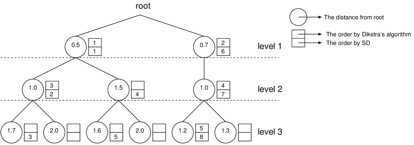
Figure 1: The order of search by Dijkstra’s algorithm and the original SD

Arranging the nodes having the same parent according to the distance needs to compute $|\hat{a}_{i}-S_{i}|^{2}$ of nodes. Instead of doing this, our algorithm considers the candidates of $\Re(\hat{a}_{t-k+1})$ and the candidates of $\Im(\hat{a}_{t-k+1})$ separately in Section 5. Then the level of tree is equal to $2t$ excluding the root, and arranging the nodes having the same parent only needs to compute $|\Re(\hat{a}_{i})-\Re(S_{i})|$ and $|\Im(\hat{a}_{i})-\Im(S_{i})|$

5 Computer simulation

In this section, we show how much the complexity of searching part is reduced by QR factorization with sort and Dijkstra’s algorithm, the complexity of preprocessing part is increased by QR factorization with sort, and the storage complexity is increased by Dijkstra’s algorithm over an uncoded multi-antenna fading channel.

The radius of sphere used by SD is defined so that

$$\Pr\{\mbox{transmit point is in sphere}\} = \Pr\{C>\left|\mbox{\boldmath{$\nu$}}\right|^{2}\}$$ (12)

$$\approx 0.99$$

where $C$ is the square of radius and $\nu$ is a vector whose element is noise at each receive antenna [5]. When there is no lattice point in sphere, we increase the radius to $C+1$, and continue until a lattice point is found.

5.1 The system model

We consider the following system model.

• The number of transmit antennas is equal to the number of receive antennas.

• The fading coefficients obey the ${\cal CN}(0,1)$ distribution.

• The signal constellation for each transmit antenna is $64$-QAM and all signals are drawn according to the uniform i.i.d. distribution.

5.2 The computer simulations

In this subsection we show comparisons of complexities of the proposed methods and other variants of SD. We remark that all methods in this subsection are ML decoding and hence the error rates of these ML decoding methods are the same. First we show the comparison of the complexities of SD not reordering decisions on $\hat{a}_{i}$ (SD), SD reordering decisions on $\hat{a}_{i}$ according to norms of basis vectors (Norm-SD) [3, 9], SD reordering decisions on $\hat{a}_{i}$ so that $\min_{1\leq i\leq t}|r_{ii}|$ is maximized (Optimal-SD) [9] and SD with the QR factorization with sort (QR sort-SD). The value of SNR is set to 26dB. In these simulations we use the average number of real multiplications and divisions for each processing as the measure of complexity, and in these simulations we use the complex multiplications that needs three real multiplications and seven real additions, and the complex divisions that needs five real multiplications, two real divisions, and nine real additions [12]. Figure 2 shows the complexity of searching part and Figure 3 shows the complexity of preprocessing part. When the number of transmit antennas is 8 the complexity of searching part is reduced about 55 percent from the original SD by QR factorization with sort. However Figure 3 shows the complexity of preprocessing part increases about 10 percent. Figure 4 shows the total complexity of SD for 10 transmissions with the same fading matrix. In this case the complexity of SD is reduced about 60 percent from the original SD by QR factorization with sort.

Figure 2: The complexity of searching part for each receiving point

Figure 3: The complexity of preprocessing part for each fading matrix

Figure 4: The complexity of SD for 10 transmissions with the same fading matrix

Next we show the comparison of the complexities of SD (SD), Dijkstra’s algorithm (Dijkstra), and both of them using QR factorization with sort (QR sort-SD, QR sort+Dijkstra).

The number of antennas is set to 8. Figure 5 shows that the complexity of searching part and Figure 6 shows the cumulative distribution of the size of priority queue with QR factorization with sort. When SNR is 26dB, the complexity of searching part is reduced about 25 percent from the original SD by Dijkstra’s algorithm, and is reduced about 65 percent from the original SD by combining QR factorization with sort and Dijkstra’s algorithm. Figure 5 also shows that Dijkstra’s algorithm is much faster than SD when SNR is low.

Figure 5: The complexity of searching part for each receiving point

Figure 6: The cumulative distribution of the size of priority queue

6 Conclusion

We proposed the QR factorization with sort and use of Dijkstra’s algorithm as methods for decreasing the computational complexity of the sphere decoder. QR factorization with sort reduces the complexity of searching part of a decoder with little increase in the complexity of preprocessing part of a decoder. Because the preprocessing part is computed once for each fading matrix and the increase in the complexity of preprocessing part is little enough, the total complexity of SD can be reduced. Dijkstra’s algorithm reduces the complexity of searching part of a decoder with increase in the storage complexity. By these reductions of the complexity, the proposed methods enable us to implement ML decoding for the multi-antenna system with a lager number of transmit antennas.

References

- [1] E. Telatar, “Capacity of multi-antenna Gaussian channels,” Europ. Trans. Telecommun., vol.10, pp.585–595, Nov. 1999.
- [2] G. J. Foschini, “Layered space-time architecture for wireless communication in a fading environment when using multi-element antennas,” Bell Labs. Tech. J., vol.1, pp.41–59, 1996.
- [3] U. Fincke and M. Pohst, “Improved methods for calculating vectors of short length in a lattice, including a complexity analysis,” Math. Comp., vol.44, pp.436–471, Apr. 1985.
- [4] E. Viterbo and J. Boutros, “A universal lattice code decoder for fading channels,” IEEE Trans. Inform. Theory, vol.45, no.5, pp.1639–1642, July 1999.
- [5] B. Hassibi and H. Vikalo, “On the sphere decoding algorithm: Part I and II,” http://www.systems.caltech.edu/EE/Faculty/babak/pubs/sphere.html.
- [6] M. O. Damen, A. Chkeif and J. C. Belfiore, “Lattice code decoder for space-time codes,” IEEE Comm. Lett., vol.36, no.5, pp.166–168, Jan. 2000.
- [7] A. M. Chan and I. Lee, “A new reduced-complexity sphere decoder for multiple antenna systems,” Proc. ICC, vol.1, pp.460–464, Apr. 2002.
- [8] D. Wubben, R. Bohnke, J. Rinas, V. Kuhn and K. D. Kammeyer, “Efficient algorithm for decoding layered space-time codes,” Electron. Lett., vol.37, pp.1348–1350, Oct. 2001.
- [9] M. O. Damen, H. E. Gamal and G. Caire, “On maximum-likelihood detection and the search for the closest lattice point,” IEEE Trans. Inform. Theory, vol.49, no.10, pp.2389-2402, Oct. 2003.
- [10] J. Stoer and R. Bulirsch, “Introduction to numerical analysis,” 2nd ed., Springer-Verlag, pp.190-197, 1983.
- [11] A. V. Aho, J. E. Hopcroft and J. D. Ullman, “Data structures and algorithms,” Chapter 6.3, Addison-Wesley, Reading Mass., 1983.
- [12] D. E. Knuth, “The art of computer programming,” Vol. 2, 2nd ed., Problem 6.41, Addison-Wesley, Reading Mass., 1981.