Self-Organised Factorial Encoding of a Toroidal Manifold

Abstract: It is shown analytically how a neural network can be used optimally to encode input data that is derived from a toroidal manifold. The case of a 2-layer network is considered, where the output is assumed to be a set of discrete neural firing events. The network objective function measures the average Euclidean error that occurs when the network attempts to reconstruct its input from its output. This optimisation problem is solved analytically for a toroidal input manifold, and two types of solution are obtained: a joint encoder in which the network acts as a soft vector quantiser, and a factorial encoder in which the network acts as a pair of soft vector quantisers (one for each of the circular subspaces of the torus). The factorial encoder is favoured for small network sizes when the number of observed firing events is large. Such self-organised factorial encoding may be used to restrict the size of network that is required to perform a given encoding task, and will decompose an input manifold into its constituent submanifolds.

1 Introduction

The purpose of this paper is to show analytically how a neural network can be used to optimally encode input data that is derived from a toroidal manifold. For simplicity, only the case of a 2-layer network is considered, and an objective function is defined [1] that measures the average ability of the network to reconstruct the state of its input layer from the state of its output layer. The optimum network parameter values must then minimise this objective function. In this paper the output state is chosen to be the vector of locations of a finite number of the neural firing events that arise when an input vector is presented to the network, and, in the limit of a single firing event, this reduces to a winner-take-all encoder network.

If the input vector is obtained from an arbitrary input probability density function (PDF), then the network would have to be optimised numerically, and a simple interpretation of its optimal parameters would not then be guaranteed. On the other hand, if the input PDF is constrained to have a simple enough form, then an analytic optimisation guarantees that the results can be interpreted. Because the purpose of this paper is mainly to interpret the nature of the optimal solution(s) that arise from the interplay between the input PDF and the network objective function, an analytic rather than a numerical approach will be used.

The detailed form of the optimum network parameters depends on the chosen input PDF, and, for simplicity, the input PDF will be chosen to define a curved manifold which is uniformly populated by all of the allowed input vectors. The shape of this manifold then determines the type of optimum solution that the network adopts. For instance, a 1-dimensional linear manifold with a uniform distribution of input vectors leads to an optimum solution in which each neuron fires only if the input lies within a small range of values, so the network behaves as a soft scalar quantiser. This result generalises to higher dimensional linear manifolds, where the network behaves as a soft vector quantiser. A more interesting type of optimum solution can occur when the manifold is curved. For instance, a circular manifold (which is a 1-dimensional manifold embedded in a 2-dimensional space) leads to an optimum solution that is analogous to the soft scalar quantiser obtained with a 1-dimensional linear manifold, but a toroidal manifold (which is a 2-dimensional manifold embedded in a 4-dimensional space) does not necessarily lead to an optimum solution that is analogous to the soft vector quantiser obtained with a 2-dimensional linear manifold.

For a 2-dimensional toroidal manifold, it is possible for the optimum solution to be constructed out of a pair of soft scalar quantisers, each of which encodes only one of the two circular manifolds that form the toroidal manifold. This is called a factorial encoder (because it breaks the input into its constituent factors, which it then encodes), as opposed to a joint encoder (which directly encodes the input, without first breaking it into its constituent factors). Because a factorial encoder splits up the overall encoding problem into a number of smaller encoding problems, which it then tackles in parallel, it requires fewer neurons than a joint encoder would have needed for the same encoding problem.

For the type of network objective function that is discussed in this paper, factorial encoding does not occur with linear manifolds. This is because the random nature of the neural firing events does not guarantee that at least one such event occurs in each of the soft scalar quantisers in a factorial encoder, and, for a linear manifold, this leads to a much larger average reconstruction error if a factorial encoder is used than if a joint encoder is used. This effect is summarised in figure 1 for a linear manifold, and in figure 2 for a toroidal manifold. Henceforth, only the toroidal case will be discussed, because it is a curved manifold which thus has interesting factorial encoding properties, whereas a linear manifold would not.

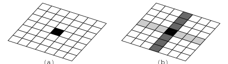
Figure 1: Diagram (a) shows the encoding cells for joint encoding of a 2-dimensional linear manifold; a typical encoding cell is shaded. Diagram (b) shows the corresponding encoding cells for a factorial encoder; typical encoding cells for each of the two factors and their intersection are shaded. The distortion that would result from only one of the two factors is large, because the encoding cell is a long thin rectangular region.

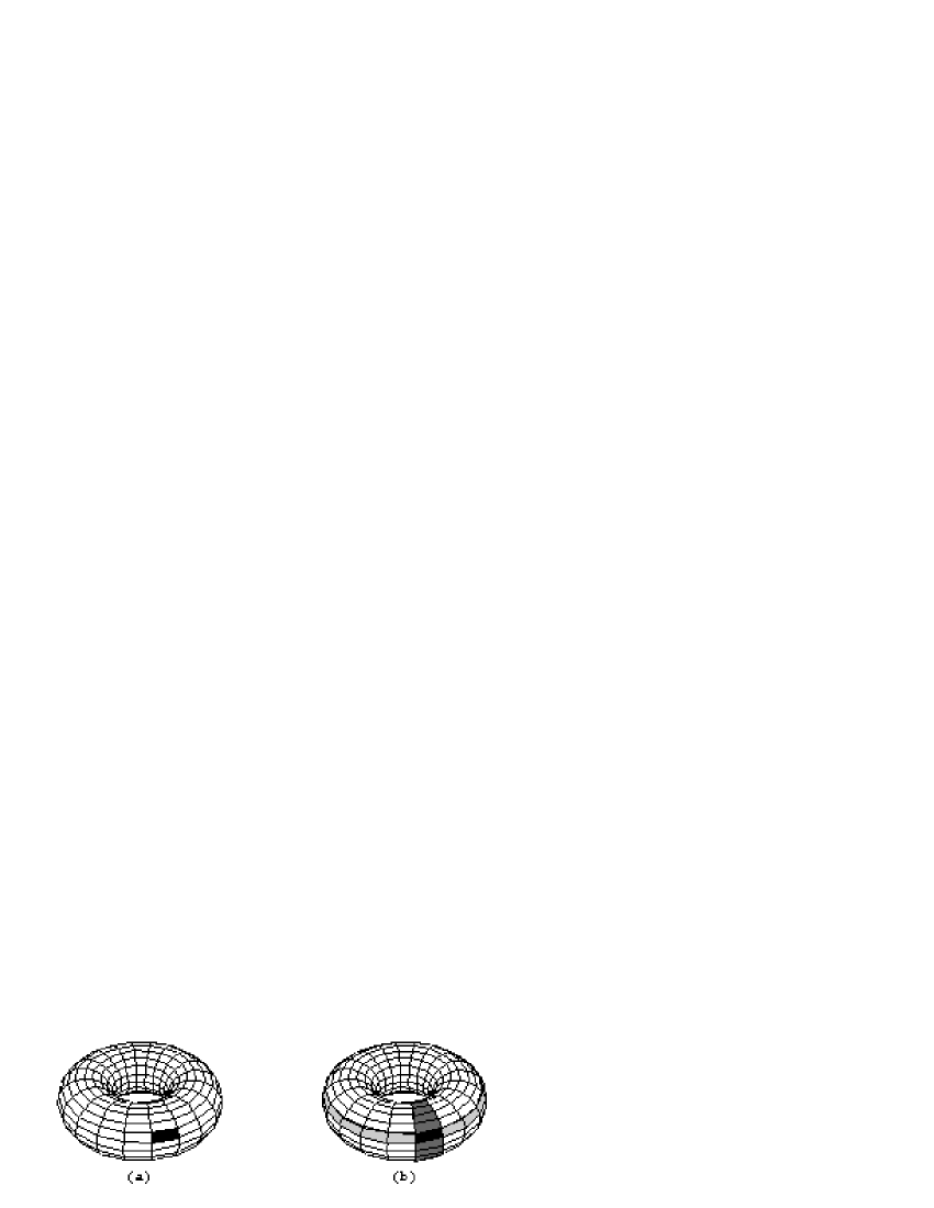
Figure 2: Diagram (a) shows the encoding cells for joint encoding of a 2-dimensional toroidal manifold; a typical encoding cell is shaded. Diagram (b) shows the corresponding encoding cells for a factorial encoder; typical encoding cells for each of the two factors and their intersection are shaded. The distortion that would result from only one of the two factors is not as large as in the case of the corresponding linear manifold, because the long thin rectangular encoding cells are now wrapped round into loops, thus reducing the average separation (in the Euclidean sense) of points within each encoding cell.

In figure 2(a) the torus is overlaid with a $20\times 20$ toroidal lattice, and a typical joint encoding cell is highlighted (this would use a total of $400=20\times 20$ neurons). Figure 2(a) makes clear why such encoding is described as “joint”, because the response of each neuron depends on the values of both dimensions of the input. The neural network implementation of this type of joint encoder would have connections from each output neuron to all of the input neurons.

In figure 2(b) the torus is overlaid with a $20\times 20$ toroidal lattice, and a typical pair of intersecting factorial encoding cells is highlighted (this would use a total of $40=20+20$ neurons). Figure 2(b) makes clear why such encoding is described as “factorial”, because the response of each neuron depends on only one of the dimensions of the input, or, in other words, on only one factor that parameterises the input space. The neural network implementation of this type of factorial encoder would have connections from each output neuron to only half of the input neurons. In figure 2(b) an accurate encoding is obtained by a process that is akin to triangulation, in which the intersection between the 2 orthogonal encoding cells defines a region of the 2-torus that is equivalent to the corresponding joint encoding cell in figure 2(a).

For a toroidal input manifold it turns out that there is an upper limit to the number of neurons that can be used if a factorial encoder is to have a smaller average reconstruction error than the corresponding joint encoder. This limit is smaller than the number of neurons that are used in figure 2(b), so that diagram should not be interpreted too literally.

1.1 Vector Quantisers

The existing literature on the simplest type of encoder (i.e. the vector quantiser (VQ)) includes the following examples:

1. A standard VQ, in which the input space is partitioned into a number of non-overlapping encoding cells, which is also known as an LBG vector quantiser (after the initials of the authors of [2]). In operation, all of the input vectors that lie closest (in the Euclidean sense) to a given code vector are assigned the same code index (which thus defines an encoding cell), and the approximate reconstruction of these inputs is then the centroid of the encoding cell. This type of VQ can be viewed as a single-layer winner-take-all (WTA) neural network.

2. A topographic VQ (TVQ), in which the code indices and encoding cells are arranged so that code indices that differ by a small amount are assigned to encoding cells that are close to each other (in the Euclidean sense). This topographic property automatically emerges if a VQ is optimised for encoding input vectors to be transmitted along a noisy communication channel [3, 4, 5, 6]. The Kohonen topographic mapping network [7] is an approximation to this type of encoder, as was explained in [5]. The TVQ may be generalised to a soft TVQ (STVQ) in which each code index is chosen probabilistically in response to the corresponding input vector [8, 9].

3. Simultaneously use more than one standard VQ, with each VQ encoding only a subspace of the input (see for example [10]); in effect, more than one code index is used to encode the input vector. By this means, a high-dimensional space can be split up into a number of lower dimensional pieces. This type of VQ is equivalent to multiple single-layer WTA neural network modules, each of which operates on a subspace of the input. This is an example of a factorial encoder, in which the input is split into a number of separate parts, or factors.

4. The simultaneous use of multiple VQs can be extended to a tree-like network of VQs [11]. This type of VQ is equivalent to multiple single layer WTA neural network modules which are connected together in a tree-like network of modules.

For simplicity, only the case of a 2-layer network (i.e. an input and an output layer) will be considered, but otherwise the network will be obliged to learn how to make use of all of its neurons. The simplest encoder which has all of the required behaviour, and which includes the above 2-layer examples as special cases, is one in which the neurons fire discretely in response to the input, and, after a finite number of firing events has occurred, the input is then reconstructed as accurately as possible (in the Euclidean sense). In the special case where only a single firing event is observed, this reduces to a standard LBG vector quantiser that was discussed in case 1 above. In the more general case, where a finite number of firing events is observed, this can lead to factorial encoder networks of the type that was discussed in case 3 above.

1.2 Curved Manifolds

The purpose of this paper is to derive optimal ways of encoding data using neural networks in which multiple firing events are observed, and to show that factorial encoder networks can be optimal when the input data lies on a curved manifold. In order to get a feel for how curved manifolds arise in image data, consider the examples shown in figure 3 and figure 4, which show the manifold generated by a single target (figure 3) and by a pair of targets (figure 4), when projected onto three neighbouring pixels (i.e. the locus of the 3-vector formed from these pixel values is plotted as the target(s) move around).

Figure 3: Manifold formed when the 1-dimensional image of a target (a Gaussian profile with a half-width of one pixel) is moved around. Only the projection $A_{i,j}$ onto the pixels at $\left(i,j\right)=\left(-1,0\right)$, $\left(0,0\right)$ and $\left(1,0\right)$ is shown.

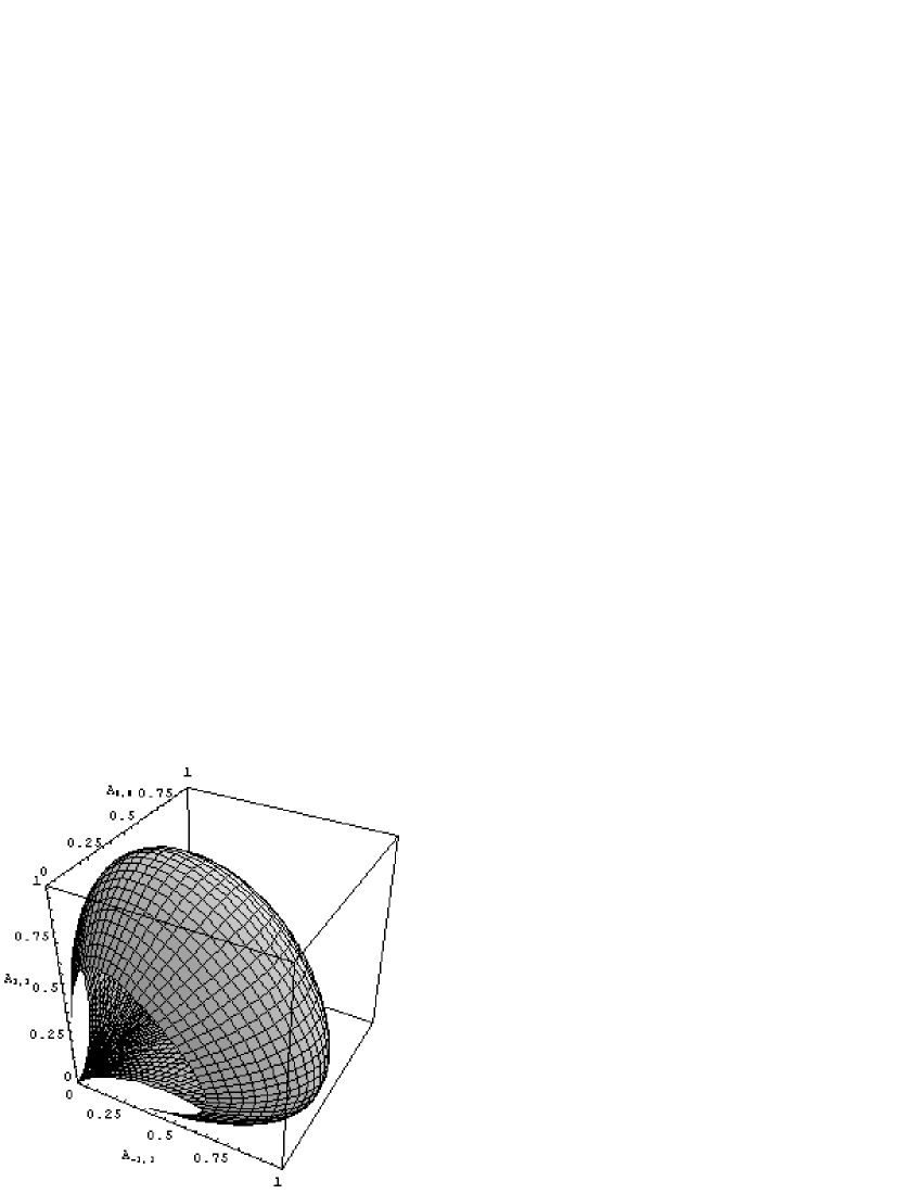
Figure 4: Manifold formed when the 2-dimensional image of a target (a Gaussian profile with half-widths of one pixel in each direction) is moved around. Only the projection $A_{i,j}$ onto the pixels at $\left(i,j\right)=\left(-1,1\right)$, $\left(0,0\right)$ and $\left(1,1\right)$ is shown.

Clearly, these image manifolds are curved, and the curvature gets greater the narrower the Gaussian profiles used to generate the target images become.

It is not at all obvious how best to encode vectors that lie on such manifolds. For instance, one might try to tile the manifold with a large number of small encoding cells obtained from some variant of a VQ, or one might try to project the manifold onto a basis obtained from some variant of principal components analysis (PCA). In fact, these two examples are both special cases of the approach that is advocated in this paper; a VQ corresponds to a single firing event, whereas PCA corresponds to an infinite number of firing events.

The problem of optimally encoding data that is derived from a general curved manifold requires a numerical solution. However, in order to develop our understanding, it is best to start with an analytically tractable example based on a simple curved manifold, which is carefully selected to preserve the essential features of more general curved manifolds. With this in mind, the most important feature to preserve in the analytic example is curvature. A circle is the simplest 1-dimensional curved manifold, which may then be used to construct higher dimensional toroidal manifolds. For instance, a pair of circles may be used to construct the 2-dimensional toroidal manifold shown in figure 2. It turns out that, if a toroidal manifold is used, then the network objective function can be analytically minimised to yield results that exhibit interesting joint encoder and factorial encoder properties.

1.3 Structure of this Paper

In section 2 the basic theoretical framework is introduced, from which some expressions are derived for optimising a network which is trained on data from a toroidal input manifold. In section 3 the detailed results for encoding a circular input manifold are given (which are trivially related to the corresponding results for the case of joint encoding of a 2-torus), and in section 4 these results are extended to the case of factorial encoding of a 2-torus. The results for joint encoding and factorial encoding are compared in section 5. Some useful asymptotic approximations are discussed in section 6, and a useful approximation to the optimal network is discussed in section 7.

The main steps in the derivations are reported in the appendices to this paper, and in several cases there is a considerable amount of algebra involved, which was done using algebraic manipulator software [12].

2 Basic Theoretical Framework

The encoder model that is assumed throughout this paper is a 2-layer network of neurons. The state of the input layer is denoted as an input vector $\mathbf{x}$ (which is assumed in this paper to be a continuous activity pattern), and the state of the output layer is denoted as the output vector $\mathbf{y}$ (which is assumed in this paper to be a discrete pattern of firing events). The information content of the output state $\mathbf{y}$ may be used to draw inferences about the input state $\mathbf{x}$. This can be formalised by using Bayes’ theorem in the form

$$\Pr\left(\mathbf{x}|\mathbf{y}\right)=\frac{\Pr\left(\mathbf{y|x}\right)\Pr\left(\mathbf{x}\right)}{\int d\mathbf{x}^{\prime}\Pr\left(\mathbf{y|x}^{\prime}\right)\Pr\left(\mathbf{x}^{\prime}\right)}$$ (1)

where the PDF $\Pr\left(\mathbf{x}|\mathbf{y}\right)$ of the input $\mathbf{x}$ given that the output $\mathbf{y}$ is known (i.e. the generative model) is completely determined by two quantities: the likelihood $\Pr\left(\mathbf{y}|\mathbf{x}\right)$ that output $\mathbf{y}$ occurs when input $\mathbf{x}$ is present (i.e. the recognition model), and the prior PDF $\Pr\left(\mathbf{x}\right)$ that input $\mathbf{x}$ could occur irrespective of whether $\mathbf{y}$ is being observed. However, for all but the most trivial situations, if the functional form of $\Pr\left(\mathbf{y|x}\right)$ is simple then the functional form of $\Pr\left(\mathbf{x}|\mathbf{y}\right)$ is complicated (or vice versa, with the roles of $\Pr\left(\mathbf{y|x}\right)$ and $\Pr\left(\mathbf{x}|\mathbf{y}\right)$ interchanged). In other words, if the recognition and generative models are strictly related by Bayes’ theorem, then difficulties inevitably arise in analytic and numerical calculations.

A possible way around this problem is to use a network objective function $D_{0}$ that has a simple functional form for the $\Pr\left(\mathbf{y|x}\right)$, but has an approximation to the ideal $\Pr\left(\mathbf{x}|\mathbf{y}\right)$ implied by Bayes’ theorem (or vice versa). A convenient choice is

$$D_{0} \equiv-\int d\mathbf{x}\sum_{\mathbf{y}}\Pr\left(\mathbf{x},\mathbf{y}\right)\log Q\left(\mathbf{x},\mathbf{y}\right)$$

$$=-\int d\mathbf{x}\Pr\left(\mathbf{x}\right)\sum_{\mathbf{y}}\Pr\left(\mathbf{y}|\mathbf{x}\right)\log Q\left(\mathbf{x}|\mathbf{y}\right)-\sum_{\mathbf{y}}\Pr\left(\mathbf{y}\right)\log Q\left(\mathbf{y}\right)$$ (2)

$\Pr\left(\mathbf{x},\mathbf{y}\right)$ is a joint probability that satisfies $\Pr\left(\mathbf{x},\mathbf{y}\right)=$ $\Pr\left(\mathbf{y|x}\right)\Pr\left(\mathbf{x}\right)=\Pr\left(\mathbf{x}|\mathbf{y}\right)\Pr\left(\mathbf{y}\right)$ (i.e. Bayes’ theorem holds), $Q\left(\mathbf{x},\mathbf{y}\right)$ is an approximation to $\Pr\left(\mathbf{x},\mathbf{y}\right)$ that satisfies the corresponding relationships $Q\left(\mathbf{x},\mathbf{y}\right)=$ $Q\left(\mathbf{y|x}\right)Q\left(\mathbf{x}\right)=Q\left(\mathbf{x}|\mathbf{y}\right)Q\left(\mathbf{y}\right)$, $\int d\mathbf{x}\Pr\left(\mathbf{x}\right)\left(\cdots\right)$ integrates over all the possible states of the input layer, $\sum_{\mathbf{y}}\Pr\left(\mathbf{y}|\mathbf{x}\right)\left(\cdots\right)$ sums over all the possible states of the output layer given that the state of the input layer is known, and $\sum_{\mathbf{y}}\Pr\left(\mathbf{y}\right)\left(\cdots\right)$ sums over all the possible states of the output layer.

The objective function $D_{0}$ measures the average number of bits required when the approximate joint probability $Q\left(\mathbf{x},\mathbf{y}\right)$ is used as a reference to encode each pair $\left(\mathbf{x},\mathbf{y}\right)$ drawn randomly from the true joint probability $\Pr\left(\mathbf{x},\mathbf{y}\right)$ [14], so $D_{0}$ belongs to the class of minimum description length (MDL) objective functions [15]. Strictly speaking, the number of bits depends on the accuracy with which the continuous-valued $\mathbf{x}$ is measured. However, this refinement is omitted from equation 2 because it does not affect the results in this paper, provided that the size of the quantisation cells into which $\mathbf{x}$ is binned is much smaller than the scale on which $\Pr\left(\mathbf{x}|\mathbf{y}\right)$ and $Q\left(\mathbf{x}|\mathbf{y}\right)$ fluctuate.

The objective function $D_{0}$ can be simplified if $Q\left(\mathbf{x},\mathbf{y}\right)$ is assumed to have the following properties

$$Q\left(\mathbf{y}\right) =\text{constant}$$

$$Q\left(\mathbf{x}|\mathbf{y}\right) =\frac{1}{\left(\sqrt{2\pi}\sigma\right)^{\dim\mathbf{x}}}\exp\left(-\frac{\left\|\mathbf{x}-\mathbf{x}^{\prime}\left(\mathbf{y}\right)\right\|^{2}}{2\sigma^{2}}\right)$$ (3)

where the approximation $Q\left(\mathbf{x}|\mathbf{y}\right)$ to the true generative model $\Pr\left(\mathbf{x}|\mathbf{y}\right)$ is a Gaussian PDF, and the prior probabilities $Q\left(\mathbf{y}\right)$ are constrained to all be equal. If the value of $\sigma$ is fixed, then $D_{0}$ may be replaced by the simpler, but equivalent, vector quantiser objective function $D_{VQ}$, which is defined as

$$D_{VQ}\equiv\int d\mathbf{x}\Pr\left(\mathbf{x}\right)\sum_{\mathbf{y}}\Pr\left(\mathbf{y}|\mathbf{x}\right)\left\|\mathbf{x}-\mathbf{x}^{\prime}\left(\mathbf{y}\right)\right\|^{2}$$ (4)

where $\sum_{\mathbf{y}}\Pr\left(\mathbf{y}\right)=1$ has been used to eliminate the $\sum_{\mathbf{y}}\Pr\left(\mathbf{y}\right)\log Q\left(\mathbf{y}\right)$ term. This measures the average Euclidean distortion that occurs when the input $\mathbf{x}$ is probabilistically encoded as $\mathbf{y}$, and then subsequently reconstructed as $\mathbf{x}^{\prime}\left(\mathbf{y}\right)$. This is a soft version of the LBG vector quantiser objective function [2], in which $\mathbf{y}$ acts as a code index, $\Pr\left(\mathbf{y}|\mathbf{x}\right)$ acts a soft encoding prescription for probabilistically transforming $\mathbf{x}$ into $\mathbf{y}$, and $\mathbf{x}^{\prime}\left(\mathbf{y}\right)$ acts as the corresponding code vector. The optimal $\Pr\left(\mathbf{y}|\mathbf{x}\right)$ that minimises $D_{VQ}$ is deterministic (i.e. each $\mathbf{x}$ is transformed to one, and only one, $\mathbf{y}$), so $D_{VQ}$ actually leads to an LBG vector quantiser itself, rather than merely a probabilistic version thereof [8].

Under the same assumptions (see equation 3) that yielded the expression for $D_{VQ}$, the Helmholtz machine objective function [13] would reduce to

$$D_{HM}=D_{VQ}+\int d\mathbf{x}\Pr\left(\mathbf{x}\right)\sum_{\mathbf{y}}\Pr\left(\mathbf{y}|\mathbf{x}\right)\log\Pr\left(\mathbf{y}|\mathbf{x}\right)$$ (5)

where the extra term is the so-called “bits-back” term, which is (minus) the entropy of the output $\mathbf{y}$ given that the input $\mathbf{x}$ is known, then averaged over all inputs. Thus $D_{HM}$ does not directly penalise $\Pr\left(\mathbf{y}|\mathbf{x}\right)$ that have a large entropy, or, in other words, it allows the recognition model $\Pr\left(\mathbf{y}|\mathbf{x}\right)$ to be such that many output states $\mathbf{y}$ are permitted once the input state $\mathbf{x}$ is known. This means that the recognition models produced by a Helmholtz machine tend to be more stochastic than they would have been had the “bits-back” term been omitted from $D_{HM}$. Conversely, the objective function $D_{VQ}$ that is used in this paper directly penalises $\Pr\left(\mathbf{y}|\mathbf{x}\right)$ that have a large entropy, so the recognition models produced tend to be more deterministic than the stochastic ones that the Helmholtz machine would produce under equivalent circumstances. Thus using $D_{VQ}$ tends to lead to sparse codes in which few neurons can fire, whereas using $D_{HM}$ tends to lead to distributed codes in which many neurons can fire.

The chosen objective function has both an information theoretic interpretation (given by $D_{0}$ in equation 2), in which it seeks to minimise the number of bits required to encode $\Pr\left(\mathbf{x},\mathbf{y}\right)$, and also an encoder/decoder interpretation (given by $D_{VQ}$ in equation 4), in which it seeks to minimise the Euclidean distortion that arises when $\mathbf{x}$ is encoded as $\mathbf{y}$ and then subsequently reconstructed as $\mathbf{x}^{\prime}\left(\mathbf{y}\right)$. Also, using $D_{VQ}$ as the network objective function ensures backward compatibility with preexisting results (e.g. [2, 7]).

An upper bound on the network objective function is introduced in section 2.1, and the stationarity conditions which must be satisfied for an optimal network behaviour are derived in section 2.2. Joint encoding on a 2-torus is discussed in section 2.3, and factorial encoding on a 2-torus is discussed in section 2.4.

2.1 Objective Function

In order to make progress it is necessary to make some assumptions about the network output state $\mathbf{y}$. Thus the output layer will be assumed to consist of $M$ neurons that fire discretely in response to the input activity pattern $\mathbf{x}$. Furthermore, $\mathbf{y}$ will be assumed to be an $n$-dimensional vector, that consists of the observations of the locations $\left(y_{1},y_{2},\cdots,y_{n}\right)$ of the first $n$ firing events that occur in response to input $\mathbf{x}$ (this is described in detail in [1]). Note that the individual $y_{i}$ are scalars, but the generalisation to vector-valued $\mathbf{y}_{i}$ is straightforward.

For compatibility with results published earlier (e.g. [8, 1]), the objective function that will be used here is $D=2D_{VQ}$, which has an upper bound $D_{1}+D_{2}$ given by (see appendix A for a detailed derivation and discussion)

$$D_{1} \equiv\frac{2}{n}\int d\mathbf{x}\Pr\left(\mathbf{x}\right)\sum_{y=1}^{M}\Pr\left(y|\mathbf{x}\right)\left\|\mathbf{x}-\mathbf{x}^{\prime}\left(y\right)\right\|^{2}$$

$$D_{2} \equiv\frac{2\left(n-1\right)}{n}\int d\mathbf{x}\Pr\left(\mathbf{x}\right)\left\|\mathbf{x}-\sum_{y=1}^{M}\Pr\left(y|\mathbf{x}\right)\mathbf{x}^{\prime}\left(y\right)\right\|^{2}$$ (6)

where $\Pr\left(y|\mathbf{x}\right)$ is the probability that neuron $y$ fires first in response to input $\mathbf{x}$, and $\mathbf{x}^{\prime}\left(y\right)$ is a reference vector that is used by neuron $y$ in its attempt to approximately reconstruct the input. In the limit $n=1$ only $D_{1}$ contributes, and a standard LBG vector quantiser emerges when $D_{1}$ is minimised. As $n\rightarrow\infty$ only $D_{2}$ contributes, and a PCA encoder emerges when $D_{2}$ is minimised.

This upper bound $D_{1}+D_{2}$ on the objective function $D$ will be used to derive all of the results in this paper. Its functional form, in which $\Pr\left(y|\mathbf{x}\right)$ appears only quadratically (unlike in equation 5 for $D_{HM}$), allows analytic results to be readily derived.

2.2 Stationarity Conditions

The upper bound $D_{1}+D_{2}$ (see equation 6) on the objective function $D=2D_{VQ}$ (see equation 4) needs to be minimised with respect to two types of parameter: posterior probabilities $\Pr\left(y|\mathbf{x}\right)$ and reference vectors $\mathbf{x}^{\prime}\left(y\right)$. This could be done numerically for an arbitrary input PDF $\Pr\left(\mathbf{x}\right)$ by using a gradient descent type of algorithm [1], but here $D_{1}+D_{2}$ will be analytically minimised for some carefully chosen special cases of $\Pr\left(\mathbf{x}\right)$.

The stationarity condition $\frac{\partial\left(D_{1}+D_{2}\right)}{\partial\mathbf{x}^{\prime}\left(y\right)}=0$ gives (see appendix B.1)

$$n\int d\mathbf{x}\Pr\left(\mathbf{x}|y\right)\,\mathbf{x=x}^{\prime}\left(y\right)+\left(n-1\right)\int d\mathbf{x}\Pr\left(\mathbf{x}|y\right)\sum_{y^{\prime}=1}^{M}\Pr\left(y^{\prime}|\mathbf{x}\right)\mathbf{x}^{\prime}\left(y^{\prime}\right)$$ (7)

where $\Pr\left(y\right)>0$ has been assumed. The $\frac{\partial\left(D_{1}+D_{2}\right)}{\partial\mathbf{x}^{\prime}\left(y\right)}=0$ stationarity condition also has the solution $\Pr\left(y\right)=0$, but this solution may be discarded because $\Pr\left(y\right)>0$ is always the case in practice. The right hand side of the stationarity condition in equation 7 has two contributions: a $D_{1}$-like contribution which is a single reference vector $\mathbf{x}^{\prime}\left(y\right)$, plus a $D_{2}$-like contribution which is $n-1$ times a sum of reference vectors $\sum_{y^{\prime}=1}^{M}\left(\int d\mathbf{x}\Pr\left(y^{\prime}|\mathbf{x}\right)\Pr\left(\mathbf{x}|y\right)\right)\mathbf{x}^{\prime}\left(y^{\prime}\right)$, where the coefficient $\int d\mathbf{x}\Pr\left(y^{\prime}|\mathbf{x}\right)\Pr\left(\mathbf{x}|y\right)$ accounts for the effect (at neuron $y$) of observing all pairs of firing events $\left(y,y^{\prime}\right)$ for $y^{\prime}=1,2,\cdots,M$. The sum of these two terms is $n$ times the total reference vector that is effectively associated with neuron $y$, which is $n$ times $\int d\mathbf{x}\Pr\left(\mathbf{x}|y\right)\,\mathbf{x}$ as given on the left hand side of equation 7.

The stationarity condition $\frac{\delta\left(D_{1}+D_{2}\right)}{\delta\log\Pr\left(y|\mathbf{x}\right)}=0$ gives (see appendix B.2)

$$\sum_{y^{\prime}=1}^{M}\left(\Pr\left(y^{\prime}|\mathbf{x}\right)-\delta_{y,y^{\prime}}\right)\,\mathbf{x}^{\prime}\left(y^{\prime}\right)\cdot\left(\frac{1}{2}\mathbf{x}^{\prime}\left(y^{\prime}\right)-n\,\mathbf{x}+\left(n-1\right)\sum_{y^{\prime\prime}=1}^{M}\Pr\left(y^{\prime\prime}|\mathbf{x}\right)\mathbf{x}^{\prime}\left(y^{\prime\prime}\right)\right)=0$$ (8)

where the constraint $\sum_{y^{\prime}=1}^{M}\Pr\left(y^{\prime}|\mathbf{x}\right)=1$ has been imposed, and $\Pr\left(\mathbf{x}\right)>0$ and $\Pr\left(y|\mathbf{x}\right)>0$ have been assumed. The $\frac{\delta\left(D_{1}+D_{2}\right)}{\delta\log\Pr\left(y|\mathbf{x}\right)}=0$ stationarity condition also has two other solutions: either $\Pr\left(\mathbf{x}\right)=0$, or $\Pr\left(\mathbf{x}\right)>0$ and $\Pr\left(y|\mathbf{x}\right)=0$. Using the normalisation constraint $\sum_{y=1}^{M}\Pr\left(y|\mathbf{x}\right)=1$, the last of these solutions ensures that $\Pr\left(y^{\prime}|\mathbf{x}\right)\leq 1$ for $y^{\prime}\neq y$, and when all values of $y$ are considered the net effect is to constrain $\Pr\left(y|\mathbf{x}\right)$ to the interval $0\leq\Pr\left(y|\mathbf{x}\right)\leq 1$, as expected.

The solutions of the stationarity condition for $\Pr\left(y|\mathbf{x}\right)$ in equation 8 are piecewise linear functions of $\mathbf{x}$. This piecewise linear property of $\Pr\left(y|\mathbf{x}\right)$ (as discussed in appendix B.2) is an enormous simplification, because it means that rather than searching the infinite dimensional space of functions $\Pr\left(y|\mathbf{x}\right)$ for the optimal ones that minimise $D_{1}+D_{2}$, one needs only search a finite dimensional space of piecewise linear functions $\Pr\left(y|\mathbf{x}\right)$ (subject to the constraints $0\leq\Pr\left(y|\mathbf{x}\right)\leq 1$ and $\sum_{y=1}^{M}\Pr\left(y|\mathbf{x}\right)=1$).

2.3 Joint Encoding

Joint encoding, as shown in figure 2(a), is characterised by a $\Pr\left(y|\mathbf{x}\right)$ in which the neurons labelled by $y$ form a discretised version of the manifold that $\mathbf{x}$ lives on. For instance, when $\mathbf{x}$ lives on a 2-torus, so that $\mathbf{x}=\left(\mathbf{x}_{1},\mathbf{x}_{2}\right)$ where $\mathbf{x}_{1}=\left(\cos\theta_{1},\sin\theta_{1}\right)$ and $\mathbf{x}_{2}=\left(\cos\theta_{2},\sin\theta_{2}\right)$, where $0\leq\theta_{1}<2\pi$ and $0\leq\theta_{2}<2\pi$, the $\Pr\left(y|\mathbf{x}\right)$ typically behave as shown in figure 2(a), where the 2-torus is tiled with encoding cells. When $n>1$ neighbouring encoding cells overlap, so figure 2(a) does not then give an accurate representation of the encoding cells.

For joint encoding of a 2-torus, $y$ must be replaced by the pair $\left(y_{1},y_{2}\right)$, where the $y_{1}$ index labels one direction around the toroidal lattice, and $y_{2}$ labels the other direction (this notation must not be confused with the $\left(y_{1},y_{2},\cdots,y_{n}\right)$ notation that was used in section 2.1). Thus $\Pr\left(y|\mathbf{x}\right)\rightarrow\Pr\left(y_{1},y_{2}|\mathbf{x}_{1},\mathbf{x}_{2}\right)$ with $1\leq y_{1}\leq\sqrt{M}$ and $1\leq y_{2}\leq\sqrt{M}$. For simplicity, assume $\Pr\left(\mathbf{x}_{1},\mathbf{x}_{2}\right)=\Pr\left(\mathbf{x}_{1}\right)\Pr\left(\mathbf{x}_{2}\right)$, where $\Pr\left(\mathbf{x}_{1}\right)$ and $\Pr\left(\mathbf{x}_{2}\right)$ each define a uniform PDF on the input manifold. The following results for $D_{1}$ and $D_{2}$ may then be derived (see appendix C.1)

$$D_{1} =\frac{4}{n}\int d\mathbf{x}_{1}\Pr\left(\mathbf{x}_{1}\right)\sum_{y_{1}=1}^{\sqrt{M}}\Pr\left(y_{1}|\mathbf{x}_{1}\right)\left\|\mathbf{x}_{1}-\mathbf{x}_{1}^{\prime}\left(y_{1}\right)\right\|^{2}$$

$$D_{2} =\frac{4\left(n-1\right)}{n}\int d\mathbf{x}_{1}\Pr\left(\mathbf{x}_{1}\right)\left\|\mathbf{x}_{1}-\sum_{y_{1}=1}^{\sqrt{M}}\Pr\left(y_{1}|\mathbf{x}_{1}\right)\,\mathbf{x}_{1}^{\prime}\left(y_{1}\right)\right\|^{2}$$ (9)

These results for $D_{1}$ and $D_{2}$ show that, under the simplifying assumptions made above, the problem of optimising a joint encoder is equivalent to the problem of optimising an encoder for $\mathbf{x}_{1}$ alone (with the replacement $M\rightarrow\sqrt{M}$), and then multiplying the value of $D_{1}+D_{2}$ by a factor 2 to account for $\mathbf{x}_{2}$ as well. This illustration of the behaviour of joint encoder posterior probabilities in the case of $\Pr\left(y_{1},y_{2}|\mathbf{x}_{1},\mathbf{x}_{2}\right)$ may readily be generalised to higher dimensions.

2.4 Factorial Encoding

Factorial encoding, as shown in figure 2(b), is characterised by a $\Pr\left(y|\mathbf{x}\right)$ in which the neurons labelled by $y$ are partitioned into a number of subsets, each of which forms a discretised version of a subspace of the manifold that $\mathbf{x}$ lives on. For instance, when $\mathbf{x}$ lives on a 2-torus, and the neurons are partitioned into two equal-sized subsets, the $\Pr\left(y|\mathbf{x}\right)$ typically behave as shown in figure 2(b), where each of the two circular subspaces within the 2-torus is tiled with encoding cells, which overlap when $n>1$.

For factorial encoding of a 2-torus $\Pr\left(y|\mathbf{x}\right)=\Pr\left(y|\mathbf{x}_{1},\mathbf{x}_{2}\right)=\frac{1}{2}\Pr\left(y|\mathbf{x}_{1}\right)+\frac{1}{2}\Pr\left(y|\mathbf{x}_{2}\right)$, where $\sum_{y=1}^{\frac{M}{2}}\Pr\left(y|\mathbf{x}_{1}\right)=1$, $\sum_{y=\frac{M}{2}+1}^{M}\Pr\left(y|\mathbf{x}_{2}\right)=1$, $\Pr\left(y|\mathbf{x}_{1}\right)=0$ for $\frac{M}{2}+1\leq y\leq M$, and $\Pr\left(y|\mathbf{x}_{2}\right)=0$ for $1\leq y\leq\frac{M}{2}$. For simplicity, assume $\Pr\left(\mathbf{x}_{1},\mathbf{x}_{2}\right)=\Pr\left(\mathbf{x}_{1}\right)\Pr\left(\mathbf{x}_{2}\right)$, where $\Pr\left(\mathbf{x}_{1}\right)$ and $\Pr\left(\mathbf{x}_{2}\right)$ each define a uniform PDF on the input manifold. The following results for $D_{1}$ and $D_{2}$ may then be derived (see appendix C.2)

$$D_{1} =\frac{2}{n}\left(\int d\mathbf{x}_{1}\Pr\left(\mathbf{x}_{1}\right)\sum_{y=1}^{\frac{M}{2}}\Pr\left(y|\mathbf{x}_{1}\right)\left\|\mathbf{x}_{1}-\mathbf{x}_{1}^{\prime}\left(y\right)\right\|^{2}+\int d\mathbf{x}_{2}\Pr\left(\mathbf{x}_{2}\right)\left\|\mathbf{x}_{2}\right\|^{2}\right)$$

$$D_{2} =\frac{4\left(n-1\right)}{n}\int d\mathbf{x}_{1}\Pr\left(\mathbf{x}_{1}\right)\left\|\mathbf{x}_{1}-\frac{1}{2}\sum_{y=1}^{\frac{M}{2}}\Pr\left(y|\mathbf{x}_{1}\right)\mathbf{x}_{1}^{\prime}\left(y\right)\right\|^{2}$$ (10)

These results for $D_{1}$ and $D_{2}$ show that, under the simplifying assumptions made above, the problem of optimising a factorial encoder is closely related to the problem of optimising two 1-dimensional encoders. This illustration of the behaviour of factorial encoder posterior probabilities in the case of $\Pr\left(y|\mathbf{x}_{1},\mathbf{x}_{2}\right)$ may readily be generalised to higher dimensions.

3 Circular Manifold

The analysis of how to encode data that lives on a curved manifold begins with the case of data that lives on a circle. In particular, assume that the input vector $\mathbf{x}$ is uniformly distributed on the unit circle centred on the origin, so that $\mathbf{x}$ can be parameterised by a single angular variable $\theta$, thus

$$\mathbf{x} =\left(\cos\theta,\sin\theta\right)$$

$$\int d\mathbf{x\,}\Pr\left(\mathbf{x}\right)\,\left(\cdots\right) =\frac{1}{2\pi}\int_{0}^{2\pi}d\theta\,\left(\cdots\right)$$ (11)

The posterior probability $\Pr\left(y|\mathbf{x}\right)$ may thus be replaced by $\Pr\left(y|\theta\right)$, and for purely conventional reasons, the range of $y$ is now chosen to be $y=0,1,\cdots,M-1$ rather than $y=1,2,\cdots,M$. The set of $M$ posterior probabilities for $y=0,1,\cdots,M-1$ can be parameterised as

$$\Pr\left(y|\theta\right)=p\left(\theta-\frac{2\pi y}{M}\right)$$ (12)

where $p\left(\theta\right)$ is the $\theta$-dependence of the posterior probability associated with the $y=0$ neuron. The $\theta$-dependence of $p\left(\theta\right)$ must be piecewise sinusoidal (i.e. made out of pieces that each have the functional form $a+b\cos\theta+c\sin\theta$) in order to ensure that $\Pr\left(y|\mathbf{x}\right)$ is piecewise linear, as is required of solutions to equation 62. Similarly, the $M$ corresponding reference vectors can be parameterised as

$$\mathbf{x}^{\prime}\left(y\right)=r\,\left(\cos\left(\frac{2\pi y}{M}\right),\sin\left(\frac{2\pi y}{M}\right)\right)$$ (13)

which all have length $r$, and thus form a regular $M$-sided polygon.

It turns out that, for input vectors that live on a circular manifold, optimal joint encoding never causes more than 3 different neurons to fire in response to a given input (i.e. no more than 3 posterior probabilities overlap in input space). This severely limits the number of different piecewise functions that have to be manipulated when solving the $D_{1}+D_{2}$ minimisation problem for input vectors that live on a circle. An analogous simplification also holds for joint and factorial encoding of a 2-torus. The case of 2 overlapping posterior probabilities can be optimised without too much difficulty, but the case of 3 overlapping posterior probabilities involves a prohibitively large amount of algebra, for which it is convenient to use an algebraic manipulator [12]. The calculations turn out to be highly structured, so the use of an algebraic manipulator could in principle be used to solve even more complicated analytic problems.

All of the results for encoding input data that lives on a circular manifold may be derived from the expression for $D_{1}+D_{2}$ in equation 6 (and the corresponding stationarity conditions), with the replacement given in equation 11 to ensure that the input manifold corresponds to a uniform distribution of data around a unit circle, and the functional forms given in equation 12 and equation 13.

The corresponding results for joint encoding of data that lives on a 2-torus can be obtained directly from these results (see section 2.3). The expression for the minimum value of $D_{1}+D_{2}$ for joint encoding a 2-torus using $\sqrt{M}\times\sqrt{M}$ neurons is obtained by making the replacement $M\rightarrow\sqrt{M}$ in the expression for the minimum value of $D_{1}+D_{2}$ for encoding a circle using $M$ neurons, and then multiplying this result by 2 in order to account for both the circles that form the 2-torus (see equation 9).

3.1 Two Overlapping Posterior Probabilities

A detailed derivation of the results reported in this section is given in appendix D.1. Because the neurons have an angular separation of $\frac{2\pi}{M}$ (see the form of the posterior probability given in equation 12), the functional form of $p\left(\theta\right)$ may be defined as

$$p\left(\theta\right)=\left\{\begin{array}[c]{ll}1&0\leq\left|\theta\right|\leq\frac{\pi}{M}-s\\ f\left(\theta\right)&\frac{\pi}{M}-s\leq\left|\theta\right|\leq\frac{\pi}{M}+s\\ 0&\left|\theta\right|\geq\frac{\pi}{M}+s\end{array}\right.$$ (14)

where the $s$ parameter is half the angular width of the overlap between the posterior probabilities of adjacent neurons on the unit circle, in which case $0\leq s\leq\frac{\pi}{M}$ ensures that no more than two neurons can respond to a given input. Anticipating the optimum solution, a typical example of this type of posterior probability is shown in figure 5.

In order to guarantee that $\Pr\left(y|\mathbf{x}\right)$ has a piecewise linear dependence on $\mathbf{x}$, as is required of solutions of equation 8, $f\left(\theta\right)$ must have the sinusoidal dependence $f\left(\theta\right)=a+b\cos\theta+c\sin\left|\theta\right|$, where the use of $\left|\theta\right|$ arises because $p\left(\theta\right)=p\left(-\theta\right)$. Note that the $\Pr\left(\mathbf{x}\right)=0$ solution to the stationarity condition on $\Pr\left(y|\mathbf{x}\right)$ (see equation 8) implies that $\Pr\left(y|\mathbf{x}\right)$ is undefined for any $\mathbf{x}$ that does not lie on the unit circle. However, for those $\mathbf{x}$ that do lie on the unit circle, the $a$, $b$ and $c$ parameters can be determined by demanding continuity of $p\left(\theta\right)$ at the ends of its piecewise intervals (i.e. at $\theta=\frac{\pi}{M}-s$ and $\theta=\frac{\pi}{M}+s$), and by demanding that the total probability of any neuron firing first is unity (i.e. the total posterior probability is normalised such that $f\left(\theta\right)+f\left(\frac{2\pi}{M}-\theta\right)=1$ in the interval $\frac{\pi}{M}-s\leq\theta\leq\frac{\pi}{M}+s$), to obtain

$$f\left(\theta\right)=\frac{1}{2}+\frac{1}{2}\frac{\sin\left(\frac{\pi}{M}-\theta\right)}{\sin s}$$ (15)

This corresponds to a piecewise linear contribution to $\Pr\left(y|\mathbf{x}\right)$ whose gradient points in the $\left(-\sin\left(\frac{\pi}{M}\right),\cos\left(\frac{\pi}{M}\right)\right)$ direction. A typical example of this type of posterior probability is shown in figure 5.

Figure 5: Plot of the optimal neural posterior probability $p\left(\theta\right)$ for $M=8$ and $n=2$. The neighbouring posterior probabilities $p\left(\theta\pm\frac{2\pi}{M}\right)$ are also plotted. The optimal value of $s$ is $s\approx 0.49\frac{\pi}{M}$. The departure of $p\left(\theta\right)$ from linearity in the interval $\frac{\pi}{M}-s\leq\theta\leq\frac{\pi}{M}+s$ is too small to be easily seen.

Without loss of generality (because the solution is symmetric under rotations of $\theta$ which are multiples of $\frac{2\pi}{M}$) set $y=0$ in equation 8, to obtain in the interval $\frac{\pi}{M}-s\leq\theta\leq\frac{\pi}{M}+s$

$$0= r\csc^{2}s\,\,\sin\left(\frac{\pi}{M}\right)\sin\left(\frac{\pi}{M}-\theta\right)\left(\sin s-\sin\left(\frac{\pi}{M}-\theta\right)\right)$$

$$\times\left(n\sin s-\left(n-1\right)\,r\sin\left(\frac{\pi}{M}\right)\right)\,\,$$ (16)

which may be solved for the optimum length $r$ of the reference vectors, to yield

$$r=\frac{n}{n-1}\frac{\sin s}{\sin\left(\frac{\pi}{M}\right)}$$ (17)

Set $y=0$ in equation 7 to obtain a transcendental equation that must be satisfied by the optimum $s$

$$\frac{\sin s}{\sin\left(\frac{\pi}{M}\right)}-\frac{n-1}{n}\frac{M}{\pi}\sin\left(\frac{\pi}{M}\right)\left(\cos s+s\sin s\right)=0$$ (18)

The symmetry of the solution may be used to make the replacement $\frac{1}{2\pi}\int_{0}^{2\pi}d\theta\,\left(\cdots\right)\rightarrow\frac{M}{\pi}\int_{0}^{\frac{\pi}{M}}d\theta\,\left(\cdots\right)$ in the expressions for $D_{1}$ and $D_{2}$, which may then be evaluated and simplified to yield the minimum $D_{1}+D_{2}$ as

$$D_{1}+D_{2}=2-\frac{n}{n-1}\frac{M}{2\pi}\left(2s+\sin\left(2s\right)\right)$$ (19)

The value of $s$ which should be used in this expression for $D_{1}+D_{2}$ is the solution of equation 18 for the chosen values of $M$ and $n$.

Note that the expression for $r$ in equation 17 and the expression for $D_{1}+D_{2}$ in equation 19 both have a finite limits as $n\rightarrow 1$, because the limiting behaviour of the solution $s$ of equation 18 is $s\rightarrow\left(n-1\right)\frac{M}{\pi}\sin^{2}\left(\frac{\pi}{M}\right)$ (see the asymptotic results in section 6), which contains a factor $n-1$ to cancel the $\frac{1}{n-1}$ factor that appears in both equation 17 and equation 19.

3.2 Three Overlapping Posterior Probabilities

A detailed derivation of the results reported in this section is given in appendix D.2. Because the neurons have an angular separation of $\frac{2\pi}{M}$, the functional form of $p\left(\theta\right)$ may be defined as

$$p\left(\theta\right)=\left\{\begin{array}[c]{ll}f_{1}\left(\theta\right)&0\leq\left|\theta\right|\leq-\frac{\pi}{M}+s\\ f_{2}\left(\theta\right)&-\frac{\pi}{M}+s\leq\left|\theta\right|\leq\frac{3\pi}{M}-s\\ f_{3}\left(\theta\right)&\frac{3\pi}{M}-s\leq\left|\theta\right|\leq\frac{\pi}{M}+s\\ 0&\left|\theta\right|\geq\frac{\pi}{M}+s\end{array}\right.$$ (20)

where the $s$ parameter is half the angular width of the overlap between the posterior probabilities of adjacent neurons on the unit circle, in which case $\frac{\pi}{M}\leq s\leq\frac{2\pi}{M}$ ensures that no more than 3 neurons can respond to a given input. Anticipating the optimum solution, a typical example of this type of posterior probability is shown in figure 6.

In order to guarantee that $\Pr\left(y|\mathbf{x}\right)$ has a piecewise linear dependence on $\mathbf{x}$, the $f_{i}\left(\theta\right)$ must have the sinusoidal dependence $f_{i}\left(\theta\right)=a_{i}+b_{i}\cos\theta+c_{i}\sin\left|\theta\right|$ for $i=1,2,3$. For those $\mathbf{x}$ that lie on the unit circle, the $a_{i}$, $b_{i}$ and $c_{i}$ parameters can be determined by imposing continuity of $p\left(\theta\right)$ at $\theta=-\frac{\pi}{M}+s$, $\theta=\frac{3\pi}{M}-s$ and $\theta=\frac{\pi}{M}+s$, and normalisation of the total posterior probability such that $f_{1}\left(\theta\right)+f_{3}\left(\frac{2\pi}{M}+\theta\right)+f_{3}\left(\frac{2\pi}{M}-\theta\right)=1$ in the interval $0\leq\theta\leq-\frac{\pi}{M}+s$, and $f_{2}\left(\theta\right)+f_{2}\left(\frac{2\pi}{M}-\theta\right)=1$ in the interval $-\frac{\pi}{M}+s\leq\theta\leq\frac{3\pi}{M}-s$. Also, to satisfy the stationarity conditions, set $y=0$ in equation 7, and also set $y=0$ in equation 8 in each of the intervals $0\leq\theta\leq-\frac{\pi}{M}+s$, $-\frac{\pi}{M}+s\leq\theta\leq\frac{3\pi}{M}-s$ and $\frac{3\pi}{M}-s\leq\theta\leq\frac{\pi}{M}+s$. These conditions are sufficient to solve for the optimum The $f_{i}\left(\theta\right)$ for $i=1,2,3$, the optimum $r$, and the optimum $s$.

The optimum $f_{i}\left(\theta\right)$ are

$$f_{1}\left(\theta\right) =-\frac{1}{4}\left(\cos\left(\frac{4\pi}{M}-s\right)+\cos s-2\cos\left(\frac{\pi}{M}\right)\cos\theta\right)\csc^{2}\left(\frac{\pi}{M}\right)\sec\left(\frac{2\pi}{M}-s\right)$$

$$f_{2}\left(\theta\right) =\frac{1}{2}\left(\cot\left(\frac{\pi}{M}\right)\sec\left(\frac{2\pi}{M}-s\right)\sin\left(\frac{\pi}{M}-\theta\right)+1\right)$$

$$f_{3}\left(\theta\right) =-\frac{1}{4}\csc^{2}\left(\frac{\pi}{M}\right)\left(\cos\left(\frac{3\pi}{M}-\theta\right)\sec\left(\frac{2\pi}{M}-s\right)-1\right)$$ (21)

which correspond to different piecewise linear contributions to $\Pr\left(y|\mathbf{x}\right)$. The $f_{1}\left(\theta\right)$ piece has a gradient that points in the $\left(1,0\right)$ direction, the $f_{2}\left(\theta\right)$ piece has a gradient that points in the $\left(-\sin\left(\frac{\pi}{M}\right),\cos\left(\frac{\pi}{M}\right)\right)$ direction, and the $f_{3}\left(\theta\right)$ piece has a gradient that points in the $\left(-\sin\left(\frac{3\pi}{M}\right),\cos\left(\frac{3\pi}{M}\right)\right)$ direction. The optimum $r$ is

$$r=\frac{n}{n-1}\frac{\cos\left(\frac{2\pi}{M}-s\right)}{\cos\left(\frac{\pi}{M}\right)}$$ (22)

and the transcendental equation that must be satisfied by the optimum $s$ (for $M=4$ this reduces to equation 18) is

$$\frac{1}{n}\frac{\cos\left(\frac{2\pi}{M}-s\right)}{\cos\left(\frac{\pi}{M}\right)}-\frac{n-1}{n}\frac{M}{\pi}\cos\left(\frac{\pi}{M}\right)\left(\sin\left(\frac{2\pi}{M}-s\right)-\left(\frac{2\pi}{M}-s\right)\cos\left(\frac{2\pi}{M}-s\right)\right)=0$$ (23)

and the minimum $D_{1}+D_{2}$ may be obtained as

$$D_{1}+D_{2}= \frac{n\,\left(\left(n-1\right)\left(2\frac{n-2}{n}-\frac{M}{\pi}\,s\right)-\sec^{2}\left(\frac{\pi}{M}\right)\right)}{2\left(n-1\right)^{2}}$$

$$-\frac{n\,\left(\left(n-1\right)\left(2-\frac{M}{\pi}\,s\right)+\sec^{2}\left(\frac{\pi}{M}\right)\right)}{2\left(n-1\right)^{2}}\cos\left(\frac{4\pi}{M}-2s\right)$$ (24)

As in section 3.1, the limit $n\rightarrow 1$ is well behaved because the limiting behaviour of the solution $s$ of equation 23 contains a factor $n-1$ (see the asymptotic results in section 6) to cancel the $\frac{1}{n-1}$ factor that appears in both equation 22 and equation 24.

Figure 6: Plot of the optimal neural posterior probability $p\left(\theta\right)$ for $M=8$ and $n=100$. The neighbouring posterior probabilities $p\left(\theta\pm\frac{2\pi}{M}\right)$ are also plotted. The optimal value of $s$ is $s\approx 1.39\frac{\pi}{M}$.

The results for the optimum value of $s$ (i.e. equation 18 and equation 23) may be combined to yield the results shown in figure 7.

Figure 7: Contour plot of the optimum value of $s$ versus $\left(n,M\right)$ for encoding of a circular manifold. The solid contours are for the interval $0\leq s<\frac{\pi}{M}$, the dotted contours are for $\frac{\pi}{M}<s\leq\frac{2\pi}{M}$, and the dashed contour is for $s=\frac{\pi}{M}$ (this behaves asymptotically as $n\approx 3\frac{M^{2}}{\pi^{2}}$). The contours are all separated by intervals of $\frac{\pi}{10M}$.

Asymptotically, as $M\rightarrow\infty$ and $n\rightarrow\infty$, the contour $s=\frac{\pi}{M}$ (the dashed line in figure 7), which is the boundary between the regions where 2 and 3 posterior probabilities overlap, is given by $n\approx 3\frac{M^{2}}{\pi^{2}}$ (see the asymptotic results in section 6).

The corresponding results for joint encoding of input vectors that live on a 2-torus are shown in figure 8.

Figure 8: Contour plot of the optimum value of $s$ versus $\left(n,M\right)$ for joint encoding of a toroidal manifold. The solid contours are for the interval $0\leq s<\frac{\pi}{\sqrt{M}}$, the dotted contours are for $\frac{\pi}{\sqrt{M}}<s\leq\frac{2\pi}{\sqrt{M}}$, and the dashed contour is for $s=\frac{\pi}{\sqrt{M}}$ (this behaves asymptotically as $n\approx 3\frac{M}{\pi^{2}}$). The contours are all separated by intervals of $\frac{\pi}{10\sqrt{M}}$.

4 Toroidal Manifold: Factorial Encoding

All of the results for factorial encoding of input data that lives on a toroidal manifold may be derived from the expression for $D_{1}+D_{2}$ in equation 10 (and the corresponding stationarity conditions), with the appropriate replacements for equations 11, 12 and 13.

The posterior probability $p\left(\theta\right)$ then has the same functional form as for a circular manifold, except that $M$ is replaced by $\frac{M}{2}$ because each of the two dimensions uses exactly half of the total of $M$ neurons, so these results are not quoted explicitly here. The steps in the derivation of the optimum values of $r$ and $s$ and the minimum value of $D_{1}+D_{2}$ are analogous to the steps that appear in the derivation for a circular input manifold, and the results are sufficiently different from the ones that were obtained from a circular manifold that they are quoted explicitly here.

4.1 Two Overlapping Posterior Probabilities

A detailed derivation of the results reported in this section is given in appendix D.3. The stationarity conditions yield the optimum $r$ as

$$r=\frac{2n}{n-1}\frac{\sin s}{\sin\left(\frac{2\pi}{M}\right)}$$ (25)

The transcendental equation that must be satisfied by the optimum $s$ is

$$\frac{\sin s}{\sin\left(\frac{2\pi}{M}\right)}-\frac{n-1}{n+1}\frac{M}{2\pi}\sin\left(\frac{2\pi}{M}\right)\ \left(\cos s+s\sin s\right)=0$$ (26)

The expression for the minimum $D_{1}+D_{2}$ is

$$D_{1}+D_{2}=4-\frac{n}{n-1}\frac{M}{2\pi}\left(2s+\sin\left(2s\right)\right)$$ (27)

4.2 Three Overlapping Posterior Probabilities

A detailed derivation of the results reported in this section is given in appendix D.4. The stationarity conditions yield the optimum $r$ as

$$r=\frac{2n}{n-1}\frac{\cos\left(\frac{4\pi}{M}-s\right)}{\cos\left(\frac{2\pi}{M}\right)}\$$ (28)

The transcendental equation that must be satisfied by the optimum $s$ is

$$\frac{1}{n}\frac{\cos\left(\frac{4\pi}{M}-s\right)}{\cos\left(\frac{2\pi}{M}\right)}-\frac{n-1}{2n}\frac{M}{2\pi}\cos\left(\frac{2\pi}{M}\right)\left(\sin\left(\frac{4\pi}{M}-s\right)-\left(\frac{4\pi}{M}-s\right)\ \cos\left(\frac{4\pi}{M}-s\right)\right)=0$$ (29)

The expression for the minimum $D_{1}+D_{2}$ is

$$D_{1}+D_{2}= \frac{n\left(\left(n-1\right)\left(2\frac{n-2}{n}\ -\frac{M}{2\pi}\,s\right)-2\sec^{2}\left(\frac{2\pi}{M}\right)\right)}{\left(n-1\right)^{2}}$$

$$-\frac{n\left(\left(n-1\right)\ \left(2-\frac{M}{2\pi}\,s\right)+2\sec^{2}\left(\frac{2\pi}{M}\right)\right)}{\left(n-1\right)^{2}}\cos\left(\frac{8\pi}{M}-2s\right)$$ (30)

The results for the optimum value of $s$ (i.e. equation 26 and equation 29) may be combined to yield the results shown in figure 9.

Figure 9: Contour plot of the optimum value of $s$ versus $\left(n,M\right)$ for factorial encoding of a toroidal manifold. The solid contours are for the interval $0\leq s<\frac{2\pi}{M}$, the dotted contours are for $\frac{2\pi}{M}<s\leq\frac{4\pi}{M}$, and the dashed contour is for $s=\frac{2\pi}{M}$ (this behaves asymptotically as $n\approx\frac{3}{2}\frac{M^{2}}{\pi^{2}}$). The contours are all separated by intervals of $\frac{\pi}{5M}$.

5 Joint Versus Factorial Encoding

The results in section 3 and section 4 may be used to deduce when a factorial encoder is favoured with respect to a joint encoder (for input data that lives on a 2-torus). Firstly, equation 18 (with the replacement $M\rightarrow\sqrt{M}$, and setting $s=\frac{\pi}{\sqrt{M}}$) may be used to deduce the region of the $\left(n,M\right)$ plane where joint encoding of a 2-torus involves no more that $2$ overlapping posterior probabilities, and equation 26 (with $s=\frac{2\pi}{M}$) may be used to deduce the corresponding result for factorial encoding of a 2-torus. Once these regions have been established, it is then possible to decide which of equation 19 or equation 24 (with $M\rightarrow\sqrt{M}$ and then multiplied overall by $2$) to use to calculate $D_{1}+D_{2}$ in the case of joint encoding a 2-torus, and which of equation 27 or equation 30 to use to calculate $D_{1}+D_{2}$ in the case of factorial encoding a 2-torus. These results are gathered together in figure 10.

Figure 10: The diagram shows various results pertaining to joint and factorial encoding of a 2-torus. The solid line is the boundary between the regions of the $\left(n,M\right)$ plane where joint or factorial encoding are favoured, and the horizontal dashed line is the asymptotic limit $M\approx 12$ of this boundary as $n\rightarrow\infty$. The left hand dashed line is the boundary between the regions where 2 or 3 overlapping posterior probabilites occur in joint encoding, and the right hand dashed line is the corresponding boundary for factorial encoding.

The need to derive results where up to 3 posterior probabilities overlap (which involves a large amount of algebra) is clear from the results shown in figure 10, where it may be seen that most of the region where the factorial encoder is favoured with respect to the joint encoder has up to 3 overlapping posterior probabilities. The degree to which a factorial encoder is favoured with respect to a joint encoder may be seen in figure 11.

Figure 11: Plots for $M=6,7,8,9,10,11$ of $\left(D_{1}+D_{2}\right)_{factorial}-\left(D_{1}+D_{2}\right)_{joint}$ in units in which $\left(D_{1}+D_{2}\right)_{factorial}=1$. This makes it clear that the degree to which a factorial encoder is favoured with respect to a joint encoder is quite significant for large $n$.

If the number of neurons $M$ is restricted (i.e. $M\lesssim 12$), then the joint encoding scheme in which the 2-torus is encoded using small encoding cells as shown in figure 2(a), is usually not as good as the factorial encoding scheme in which the 2-torus is encoded using the intersection of pairs of elongated encoding cells as shown in figure 2(b). This does require that the number of firing events $n$ is sufficiently large that both subsets of $\frac{M}{2}$ neurons in the factorial encoder are virtually guaranteed to each receive at least 1 firing event, so that they can indeed approximate the input vector by the intersection of a pair of response regions.

If the number of neurons $M$ is too large (i.e. $M\gtrsim 12$), then the joint encoding scheme is always favoured with respect to the factorial encoding scheme, because there are sufficient neurons to encode the 2-torus well using small response regions, as shown in figure 2(a). This includes the limiting case $M\rightarrow\infty$, where the curvature of the input manifold is not visible to each neuron separately, because each neuron then responds to an infinitesimally small angular interval of the input manifold. This result implies that joint encoding is always favoured when the input manifold is planar, as was discussed in figure 1 and figure 2.

Although not presented here, these results generalise readily to higher dimensional toruses, where factorial encoding is even more favoured, because (roughly speaking) the number of neurons required to do joint encoding with a given resolution increases exponentially with the dimensionality of the input, whereas the number of neurons required to do factorial encoding with a given resolution increases linearly with the dimensionality of the input (provided that enough firing events are observed).

6 Asymptotic Results

Referring to figure 10, the asymptotic behaviour as $M\rightarrow\infty$ lies in the region where two posterior probabilities overlap, and the asymptotic behaviour as $n\rightarrow\infty$ lies in the region where three posterior probabilities overlap, so care must be taken to use the appropriate results when deriving the various asymptotic approximations below. The boundary between the regions where two or three posterior probabilities overlap can be obtained for a circular input manifold by putting $s=\frac{\pi}{M}$ in equation 18 (or $s=\frac{2\pi}{M}$ in equation 26 in the case of a toroidal input manifold), and as $M\rightarrow\infty$ this is given by

$$n\approx\left\{\begin{array}[c]{ll}3\frac{M^{2}}{\pi^{2}}&\text{circular manifold}\\ \frac{3}{2}\frac{M^{2}}{\pi^{2}}&\text{toroidal manifold (factorial encoding)}\end{array}\right.$$ (31)

As $M\rightarrow\infty$ the asymptotic behaviour of $D_{1}+D_{2}$ for a circular input manifold may be obtained by asymptotically expanding the $s$ dependence of equation 18 (or equation 26 in the case of a toroidal input manifold) in inverse powers of $M$, to yield

$$s\approx\left\{\begin{array}[c]{ll}\frac{n-1}{n}\frac{\pi}{M}+\frac{(n-1)(n^{2}-4n+2)}{3n^{3}}\frac{\pi^{3}}{M^{3}}&\text{circular manifold}\\ \frac{n-1}{n+1}\frac{2\ \pi}{M}+\frac{\ (n-1)(n^{2}-6n+1)}{3(n+1)^{3}}\left(\frac{2\ \pi}{M}\right)^{3}&\text{toroidal manifold (factorial encoding)}\end{array}\right.$$ (32)

and substituting this solution into the appropriate expression for $r$ to obtain

$$r\approx\left\{\begin{array}[c]{ll}1+\frac{(2n^{2}-6n+3)}{6n^{2}}\frac{\pi^{2}}{M^{2}}&\text{circular manifold}\\ \vskip 12.0pt plus 4.0pt minus 4.0pt\frac{2n}{n+1}+\frac{8n(n^{2}-4n+1)}{3(n+1)^{3}}\frac{\pi^{2}}{M^{2}}&\text{toroidal manifold (factorial encoding)}\end{array}\right.$$ (33)

and substituting this solution into the appropriate expression for $D_{1}+D_{2}$ to obtain

$$D_{1}+D_{2}\approx\left\{\begin{array}[c]{ll}\frac{2(2n-1)\ }{3n^{2}}\frac{\pi^{2}}{M^{2}}&\text{circular manifold}\\ \frac{4}{n+1}+\frac{64n^{2}}{3(n+1)^{3}}\frac{\ \pi^{2}}{M^{2}}&\text{toroidal manifold (factorial encoding)}\end{array}\right.$$ (34)

The asymptotic result for a circular manifold may be used to determine the corresponding result for a linear manifold. Thus, if lengths are scaled so that the separation of the neurons (as measured around the circular manifold) becomes unity, which requires that all lengths are divided by $\frac{2\ \pi}{M}$, then asymptotically as $M\rightarrow\infty$ the circular manifold solution becomes identical to the solution for a linear manifold with neurons separated by unit distance. Thus the optimum solution for a linear manifold with neurons separated by unit distance is $s=\frac{n-1}{2n}$ and $D_{1}+D_{2}=\frac{2n-1\ }{6n^{2}}$ (note that $D_{1}+D_{2}$ has the dimensions of $\left(\text{length}\right)^{2}$).

As $n\rightarrow 1$ (i.e. the LBG vector quantiser limit) the asymptotic behaviour of $D_{1}+D_{2}$ for a circular input manifold may be obtained by expanding the $s$ dependence of equation 18 about the point $s=0$ (or equation 26 about the point $s=0$ for a toroidal input manifold), to yield

$$s\approx\left\{\begin{array}[c]{ll}\left(n-1\right)\frac{M}{\pi}\sin^{2}\left(\frac{\pi}{M}\right)&\text{circular manifold}\\ \frac{n-1}{2}\frac{M}{2\pi}\sin^{2}\left(\frac{2\pi}{M}\right)&\text{toroidal manifold (factorial encoding)}\end{array}\right.$$ (35)

which gives $s=0$ when $n=1$, so there is no overlap between the posterior probabilities for different neurons, as would be expected in a vector quantiser where only one neuron is allowed to fire. Substitute this solution into the appropriate expression for $r$ to obtain at $n=1$

$$r=\left\{\begin{array}[c]{ll}\frac{M}{\pi}\sin\left(\frac{\pi}{M}\right)&\text{circular manifold}\\ \frac{M\ }{2\pi}\sin\left(\frac{2\pi}{M}\right)&\text{toroidal manifold (factorial encoding)}\end{array}\right.$$ (36)

which is the distance of the centroid of an arc of the unit circle (with angular length $\frac{2\pi}{M}$ for a circular manifold, or angular length $\frac{4\pi}{M}$ for a toroidal manifold) from the origin, as expected for a network in which only one neuron can fire. So the best reconstruction is the centroid of the inputs that could have caused the single firing event. These results may be substituted into the appropriate expression for $D_{1}+D_{2}$ to obtain at $n=1$

$$D_{1}+D_{2}=\left\{\begin{array}[c]{ll}2-2\left(\frac{M}{\pi}\right)^{2}\sin^{2}\left(\frac{\pi}{M}\right)&\text{circular manifold}\\ 4-2\left(\frac{M}{2\pi}\right)^{2}\sin^{2}\left(\frac{2\pi}{M}\right)&\text{toroidal manifold (factorial encoding)}\end{array}\right.$$ (37)

These results for $D_{1}+D_{2}$ have a simple geometrical interpretation. For a circular manifold $D_{1}+D_{2}$ is (twice) the average squared distance from an arc with angular length $\frac{2\pi}{M}$ to its associated reference vector, which is exactly what would be expected. For a toroidal manifold $D_{1}+D_{2}$ is the same result with $M\rightarrow\frac{M}{2}$, plus an extra contribution of 2, because a factorial encoder with only 1 firing event acts as a conventional encoder using $\frac{M}{2}$ neurons for the circular dimension that is fortunate enough to be associated with the firing event (hence the first contribution to $D_{1}+D_{2}$), and acts as no encoder at all for the other circular dimension which is associated with no firing events (hence the extra contribution of 2 to $D_{1}+D_{2}$).

As $n\rightarrow\infty$ the asymptotic behaviour of $D_{1}+D_{2}$ for a circular input manifold may be obtained by expanding the $s$ dependence of equation 23 about the point $s=\frac{2\pi}{M}$ (or equation 29 about the point $s=\frac{4\pi}{M}$ for a toroidal input manifold), to yield

$$s\approx\left\{\begin{array}[c]{ll}\frac{2\pi}{M}-\left(\frac{3\pi}{M\,n\cos^{2}\left(\frac{\pi}{M}\right)}\right)^{\frac{1}{3}}&\text{circular manifold}\\ \frac{4\pi}{M}-\left(\frac{12\pi}{M\,n\cos^{2}\left(\frac{2\pi}{M}\right)}\right)^{\frac{1}{3}}&\text{toroidal manifold (factorial encoding)}\end{array}\right.$$ (38)

where the limiting values of $s$ as $n\rightarrow\infty$ (i.e. $s\rightarrow\frac{2\pi}{M}$ for a circular manifold, and $s\rightarrow\frac{4\pi}{M}$ for a toroidal manifold) stops just short of allowing four or more posterior probabilities to overlap. In this limit $D_{1}=0$, so for a circular manifold the network acts as a PCA encoder (see the discussion after equation 6) whose expansion coefficients sum to unity. In order to encode vectors on a unit circle without error three basis vectors are required; the expansion coefficients are probabilities which must sum to unity, so three basis vectors are required in order that there are two independent expansion coefficients. This is the reason why it is sufficient to consider no more than three overlapping posterior probabilities for encoding data that lives in a 2-dimensional manifold (this argument generalises straightforwardly to higher dimensions). The same argument applies to the case of factorial encoding of a toroidal manifold. Substitute this solution into the appropriate expression for $r$ to obtain

$$r\approx\left\{\begin{array}[]{cc}\frac{1}{2}\sec(\frac{\pi}{\mathit{M}})\left(2-{\left(\frac{3\pi}{\mathit{M}\mathit{n}{\cos}^{2}(\frac{\pi}{\mathit{M}})}\right)}^{2/3}\right)&\mathrm{circular}\;\mathrm{manifold}\\ \sec(\frac{2\pi}{\mathit{M}})\left(2-{\left(\frac{12\pi}{\mathit{M}\mathit{n}{\cos}^{2}(\frac{2\pi}{\mathit{M}})}\right)}^{2/3}\right)&\mathrm{toroidal}\;\mathrm{manifold}\left(\mathrm{factorial}\;\mathrm{encoding}\right)\end{array}\right.$$ (39)

and substitute these results into the appropriate expression for $D_{1}+D_{2}$ to obtain

$$D_{1}+D_{2}\approx\left\{\begin{array}[c]{ll}\frac{2\ }{n}\tan^{2}\left(\frac{\pi}{M}\right)&\text{circular manifold}\\ \frac{4}{n}\left(2\sec^{2}\left(\frac{2\ \pi}{M}\right)-1\right)&\text{toroidal manifold (factorial encoding)}\end{array}\right.$$ (40)

Thus as $n\rightarrow\infty$ it is possible to derive a value of $M$ for which the asymptotic $D_{1}+D_{2}$ is the same for joint and factorial encoding of a toroidal manifold. This value of $M$ must satisfy $\frac{4\ }{n}\tan^{2}\left(\frac{\pi}{\sqrt{M}}\right)=\frac{4}{n}\left(2\sec^{2}\left(\frac{2\ \pi}{M}\right)-1\right)$, which yields $M\approx 11.74$.

7 Approximate the Posterior Probability

A posterior probability may always be written in the form

$$\Pr\left(y|\mathbf{x}\right)=\frac{Q\left(\mathbf{x}|y\right)}{\sum_{y^{\prime}=0}^{M-1}Q\left(\mathbf{x}|y^{\prime}\right)}$$ (41)

where $Q\left(\mathbf{x}|y\right)\geq 0$ (with $Q\left(\mathbf{x}|y\right)>0$ for at least one value of $y$ for each $\mathbf{x}$). If the neurons behaved in such a way that they produced independent Poissonian firing events in response to a given input, then $Q\left(\mathbf{x}|y\right)$ would be the firing rate (or activation function) of neuron $y$ in response to input $\mathbf{x}$.

The optimum solution $p\left(\theta\right)$ (as given in equation 14 and equation 15) may be approximated on the unit circle (i.e. $\mathbf{x}=\left(\cos\theta,\sin\theta\right)$) by defining $Q\left(\mathbf{x}|y\right)$ as

$$Q\left(\mathbf{x}|y\right) =\left\{\begin{array}[c]{ll}\mathbf{w}\cdot\mathbf{x}-a&\mathbf{w}\cdot\mathbf{x}\geq a\\ 0&\mathbf{w}\cdot\mathbf{x}\leq a\end{array}\right.$$ (44)

$$\mathbf{w} =\left(\cos\left(\frac{2\pi y}{M}\right),\sin\left(\frac{2\pi y}{M}\right)\right)$$

$$a =\cos\left(\frac{\pi}{M}\right)-\sin\left(\frac{\pi}{M}\right)\sin s$$ (45)

where $a$ is a threshold parameter, and $\mathbf{w}$ is a unit weight vector. This is the form of the neural activation function that is used in [16]. This leads to a good approximation to the optimum solution $p\left(\theta\right)$ because

$$p\left(\theta\right)=\left\{\begin{array}[c]{ll}0&\theta\leq-\frac{\pi}{M}-s\\ \frac{Q\left(\mathbf{x}|y=0\right)}{Q\left(\mathbf{x}|y=0\right)+Q\left(\mathbf{x}|y=M-1\right)}+O\left(\left(\theta+\frac{\pi}{M}\right)^{3}\right)&-\frac{\pi}{M}-s\leq\theta\leq-\frac{\pi}{M}+s\\ 1&-\frac{\pi}{M}+s\leq\theta\leq\frac{\pi}{M}-s\\ \frac{Q\left(\mathbf{x}|y=0\right)}{Q\left(\mathbf{x}|y=0\right)+Q\left(\mathbf{x}|y=1\right)}+O\left(\left(\theta-\frac{\pi}{M}\right)^{3}\right)&\frac{\pi}{M}-s\leq\theta\leq\frac{\pi}{M}+s\\ 0&\theta\geq\frac{\pi}{M}+s\end{array}\right.$$ (46)

This approximation works well because curved input manifolds can be optimally encoded by using appropriate hyperplanes (as defined in equation 45) to slice off pieces of the manifold.

This approximation breaks down as $M\longrightarrow\infty$, as can be seen by inspecting the series expansion of $p\left(\theta\right)$ near $\theta=\frac{\pi}{M}$.

$$p\left(\theta\right)=\left\{\begin{array}[c]{ll}\begin{array}[c]{l}\frac{1}{2}-\frac{1}{2}\frac{1}{\sin s}\left(\theta-\frac{\pi}{M}\right)+\frac{1}{12}\frac{1}{\sin s}\left(\theta-\frac{\pi}{M}\right)^{3}\\ +O\left(\left(\theta-\frac{\pi}{M}\right)^{4}\right)\end{array}&\text{exact}\\ \begin{array}[c]{l}\frac{1}{2}-\frac{1}{2}\frac{1}{\sin s}\left(\theta-\frac{\pi}{M}\right)+\frac{1}{12}\left(\frac{1}{\sin s}-\frac{3}{\tan\frac{\pi}{M}\sin^{2}s}\right)\left(\theta-\frac{\pi}{M}\right)^{3}\\ +O\left(\left(\theta-\frac{\pi}{M}\right)^{4}\right)\end{array}&\text{approximate}\end{array}\right.$$ (47)

which differ in the $O\left(\left(\theta-\frac{\pi}{M}\right)^{3}\right)$ term. In the limit $M\longrightarrow\infty$ the half-width parameter $s$ behaves like $M^{-1\,}$, so the $O\left(\left(\theta-\frac{\pi}{M}\right)^{3}\right)$ term behaves like $M\left(\theta-\frac{\pi}{M}\right)^{3}$ in the exact case, and  $M^{3}\left(\theta-\frac{\pi}{M}\right)^{3}$ in the approximate case because of the contribution from the $\frac{3}{\tan\frac{\pi}{M}\sin^{2}s}$ term. As $M\longrightarrow\infty$ each neuron responds to a progressively smaller angular range of inputs on the unit circle, so from the point of view of each neuron the curvature of the input manifold becomes negligible (i.e. the input manifold appears to more and more closely approximate a straight line), which ultimately makes it impossible to use hyperplanes to slice off pieces of the manifold. In the $M\longrightarrow\infty$ limit, a better approximation to the posterior probability would be to use ball-shaped regions (e.g. a radial basis function network) to cut up the input manifold into pieces.

8 Conclusions

The results in this paper demonstrate that, for input data that lies on a curved manifold (specifically, a 2-torus), and for an objective function that measures the average reconstruction error (in the Euclidean sense) of a 2-layer neural network encoder, the type of encoder that is optimal depends on the total number of neurons and on the total number of observed firing events in the network output layer. There are two basic types of encoder: a joint encoder in which the network acts as a vector quantiser for the whole input space, and a factorial encoder in which the network breaks into a number of subnetworks, each of which acts as a vector quantiser for a subspace of the input space.

The particular conditions under which factorial encoding is favoured with respect to joint encoding arise when the input data is derived from a curved input manifold, provided that the number of neurons is not too large, and provided that the number of observed neural firing events is large enough. Factorial encoding does not emerge when the input manifold is insufficiently curved, or equivalently when there are too many neurons, because then each neuron does not have a sufficiently large encoding cell to be aware of the manifold’s curvature.

Factorial encoding allows the input data to be encoded using a much smaller number of neurons than would be the case if joint encoding were used. Because only a small number of neurons is used, a factorial encoding scheme must be succinct, so it has to abstract the underlying degrees of freedom in the input manifold; this is a very useful side-effect of factorial encoding. This effect becomes stronger as the dimensionality of the curved input manifold is increased.

The main simplification that makes these calculations possible is that, in an optimal neural network, the form for the posterior probability is a piecewise linear function of the input vector. This leads to an enormous simplification in the mathematics, because only the space of piecewise linear functions needs to be searched for the optimal solution, rather than the whole space of functions (subject to normalisation and non-negativity constraints).

A convenient approximation to this type of factorial encoder is the partitioned mixture distribution (PMD) network [17], in which the individual subnetworks in the factorial encoder network are constrained to share parameters, which thus leads to an upper bound on the minimum value of the objective function that would have ideally been obtained with the unconstrained factorial encoder network.

9 Acknowledgements

I thank Chris Webber for many useful conversations that we had during the course of this research.

Appendix A Objective Function

The objective function $D=2D_{VQ}$ is given by

$$D\equiv 2\int d\mathbf{x}\Pr\left(\mathbf{x}\right)\sum_{\mathbf{y}}\Pr\left(\mathbf{y}|\mathbf{x}\right)\left\|\mathbf{x}-\mathbf{x}^{\prime}\left(\mathbf{y}\right)\right\|^{2}$$ (48)

If the observed state of the output layer is the locations of $n$ firing events on $M$ neurons, then this expression for $D$ can be manipulated into the following form [1]

$$D=2\int d\mathbf{x}\Pr\left(\mathbf{x}\right)\sum_{y_{1}=1}^{M}\sum_{y_{2}=1}^{M}\cdots\sum_{y_{n}=1}^{M}\Pr\left(y_{1},y_{2},\cdots,y_{n}|\mathbf{x}\right)\left\|\mathbf{x}-\mathbf{x}^{\prime}\left(y_{1},y_{2},\cdots,y_{n}\right)\right\|^{2}$$ (49)

where $\Pr\left(\mathbf{y}|\mathbf{x}\right)$ has now been replaced by the more explicit notation $\Pr\left(y_{1},y_{2},\cdots,y_{n}|\mathbf{x}\right)$, and $\mathbf{x}^{\prime}\left(y_{1},y_{2},\cdots,y_{n}\right)$ is a vector given by

$$\mathbf{x}^{\prime}\left(y_{1},y_{2},\cdots,y_{n}\right)=\int d\mathbf{x}\Pr\left(\mathbf{x}|y_{1},y_{2},\cdots,y_{n}\right)\,\mathbf{x}$$ (50)

where $\Pr\left(\mathbf{x}|y_{1},y_{2},\cdots,y_{n}\right)$ may be expressed in terms of $\Pr\left(\mathbf{x}\right)$ and $\Pr\left(y_{1},y_{2},\cdots,y_{n}|\mathbf{x}\right)$ by using Bayes’ theorem in equation 1. The goal now is to minimise the expression for $D$ in equation 49 with respect to the function $\Pr\left(y_{1},y_{2},\cdots,y_{n}|\mathbf{x}\right)$. The correct value for $\mathbf{x}^{\prime}\left(y_{1},y_{2},\cdots,y_{n}\right)$ may be determined by treating it as an unknown parameter that has to be adjusted to minimise $D$.

$\Pr\left(y_{1},y_{2},\cdots,y_{n}|\mathbf{x}\right)$ may be interpreted as a recognition model which transforms the state of the input layer into (a probabilistic description of) the state of the output layer, and $\mathbf{x}^{\prime}\left(y_{1},y_{2},\cdots,y_{n}\right)$ may be regarded as the corresponding generative model that transforms the state of the output layer into (an approximate reconstruction of) the state of the input layer.

There is so much flexibility in the choice of $\Pr\left(y_{1},y_{2},\cdots,y_{n}|\mathbf{x}\right)$ (and the corresponding $\mathbf{x}^{\prime}\left(y_{1},y_{2},\cdots,y_{n}\right)$) that even if $D$ is minimised, it does not necessarily yield an encoded version of the input that is easily interpretable. One way in which a code can be encouraged to have a simple interpretation is to force $\mathbf{x}^{\prime}\left(y_{1},y_{2},\cdots,y_{n}\right)$ (i.e. the generative model) to be parameterised thus [1]

$$\mathbf{x}^{\prime}\left(y_{1},y_{2},\cdots,y_{n}\right)=\mathbf{x}^{\prime}\left(y_{1}\right)+\mathbf{x}^{\prime}\left(y_{2}\right)+\cdots+\mathbf{x}^{\prime}\left(y_{n}\right)$$ (51)

which is a (symmetric) superposition of reference vectors $\mathbf{x}^{\prime}\left(y\right)$ from each neuron $y$ that has been observed to fire. In this case each neuron has a clearly identifiable contribution to the reconstruction of the input, which makes it much easier to interpret what each neuron is doing.  In this case the $\left\|\cdots\right\|^{2}$ term in $D$ is symmetric under interchange of the $\left(y_{1},y_{2},\cdots,y_{n}\right)$, so only the symmetric part $S\left[\Pr\left(y_{1},y_{2},\cdots,y_{n}|\mathbf{x}\right)\right]$ of $\Pr\left(y_{1},y_{2},\cdots,y_{n}|\mathbf{x}\right)$ under interchange of the $\left(y_{1},y_{2},\cdots,y_{n}\right)$ contributes to $D$, because the symmetric summation $\sum_{y_{1}=1}^{M}\sum_{y_{2}=1}^{M}\cdots\sum_{y_{n}=1}^{M}\left(\cdots\right)$ then removes all non-symmetric contributions.

Define the marginal probabilities $\Pr\left(y_{1}|\mathbf{x}\right)$ and $\Pr\left(y_{1},y_{2}|\mathbf{x}\right)$ of the symmetric part $S\left[\Pr\left(y_{1},y_{2},\cdots,y_{n}|\mathbf{x}\right)\right]$ of $\Pr\left(y_{1},y_{2},\cdots,y_{n}|\mathbf{x}\right)$ under interchange of the $\left(y_{1},y_{2},\cdots,y_{n}\right)$ as

$$\Pr\left(y_{1}|\mathbf{x}\right) =\sum_{y_{2},y_{3},y_{4},\cdots,y_{n}=1}^{M}S\left[\Pr\left(y_{1},y_{2},\cdots,y_{n}|\mathbf{x}\right)\right]$$

$$\Pr\left(y_{1},y_{2}|\mathbf{x}\right) =\sum_{y_{3},y_{4},\cdots,y_{n}=1}^{M}S\left[\Pr\left(y_{1},y_{2},\cdots,y_{n}|\mathbf{x}\right)\right]$$ (52)

These marginal probabilities are for the case where $n$ firing events have potentially been observed, but only the locations of 1 (or 2) firing event(s) chosen randomly from the total number $n$ have actually been observed, with the locations of the other $n-1$ (or $n-2$) firing events having been averaged over.

If it is assumed that $\Pr\left(y_{1}|\mathbf{x}\right)$ and $\Pr\left(y_{1},y_{2}|\mathbf{x}\right)$ are related by

$$\Pr\left(y_{1},y_{2}|\mathbf{x}\right)=\Pr\left(y_{1}|\mathbf{x}\right)\Pr\left(y_{2}|\mathbf{x}\right)$$ (53)

then the objective function $D$ has an upper bound $D_{1}+D_{2}$ given by [1]

$$D \leq D_{1}+D_{2}$$

$$D_{1} \equiv\frac{2}{n}\int d\mathbf{x}\Pr\left(\mathbf{x}\right)\sum_{y=1}^{M}\Pr\left(y|\mathbf{x}\right)\left\|\mathbf{x}-\mathbf{x}^{\prime}\left(y\right)\right\|^{2}$$

$$D_{2} \equiv\frac{2\left(n-1\right)}{n}\int d\mathbf{x}\Pr\left(\mathbf{x}\right)\left\|\mathbf{x}-\sum_{y=1}^{M}\Pr\left(y|\mathbf{x}\right)\mathbf{x}^{\prime}\left(y\right)\right\|^{2}$$ (54)

Each of the two marginal probabilities in equation 52 contributes to a different term in $D_{1}+D_{2}$; $\Pr\left(y_{1}|\mathbf{x}\right)$ contributes to $D_{1}$, whereas $\Pr\left(y_{1},y_{2}|\mathbf{x}\right)$ contributes to $D_{2}$. Informally speaking, $D_{1}$ measures the information that a single firing event (out of $n$ such events) contributes to the reconstruction of the input, whereas $D_{2}$ measures the information that pairs of firing events (out of $n$ such events) contribute to the reconstruction of the input. $D_{1}$ is weighted by a factor $\frac{1}{n}$ which suppresses the single firing event contribution as $n\rightarrow\infty$, whereas $D_{2}$ is weighted by a factor $\frac{n-1}{n}$ which suppresses the double firing event contribution as $n\rightarrow 1$, as expected. If only the $D_{1}$ part of the objective function is used (i.e. $n=1$), then a standard LBG vector quantiser [2] emerges which approximates the input by a single reference vector $\mathbf{x}^{\prime}\left(y\right)$, whereas if only the $D_{2}$ part of the objective function is used (i.e. $n\rightarrow\infty$), then the network behaves essentially as a principal component analyser (PCA) which approximates the input by a sum of reference vectors $\sum_{y=1}^{M}\Pr\left(y|\mathbf{x}\right)\mathbf{x}^{\prime}\left(y\right)$, where the $\Pr\left(y|\mathbf{x}\right)$ are expansion coefficients which sum to unity, and the $\mathbf{x}^{\prime}\left(y\right)$ are basis vectors.

The upper bound $D_{1}+D_{2}$ on $D$ contains LBG encoding and PCA encoding as two limiting cases, and gives a principled way of interpolating between these extremes. This useful property has been bought at the cost of replacing $D$ by an upper bound bound $D_{1}+D_{2}$, which will yield only a suboptimal (from the point of view of $D$) encoder. However, this upper bound can be expected to be tight in cases where the input manifold can be modelled accurately using the parameteric form $\mathbf{x}^{\prime}\left(y_{1}\right)+\mathbf{x}^{\prime}\left(y_{2}\right)+\cdots+\mathbf{x}^{\prime}\left(y_{n}\right)$. These conditions are well approximated in images which consist of a discrete number of constituents, each of which may be represented by an $\mathbf{x}^{\prime}\left(y\right)$ for some choice of $y$. This model fails in situations where two or more constituents are placed so that they overlap, in which case the image will typically contain occluded objects, whereas the model assumes that the objects linearly superpose. Occlusion is not an easy situation to model, so it will be assumed that the image constituents are sufficiently sparse that they rarely occude each other.

Appendix B Stationarity Conditions

The expression for $D_{1}+D_{2}$ (see equation 6) has two types of parameters that need to be optimised: the reference vectors $\mathbf{x}^{\prime}\left(y\right)$ and the posterior probabilities $\Pr\left(y|\mathbf{x}\right)$. In appendix B.1 the stationarity condition for $\mathbf{x}^{\prime}\left(y\right)$ is derived, and in appendix B.2 the stationarity condition for $\Pr\left(y|\mathbf{x}\right)$ is derived, taking into account the constraints $0\leq\Pr\left(y|\mathbf{x}\right)\leq 1$ and $\sum_{y=1}^{M}\Pr\left(y|\mathbf{x}\right)=1$ which must be satisfied by probabilities.

B.1 Stationary $\mathbf{x}^{\prime}\left(y\right)$

The stationarity condition $\frac{\partial\left(D_{1}+D_{2}\right)}{\partial\mathbf{x}^{\prime}\left(y\right)}=0$ for $\mathbf{x}^{\prime}\left(y\right)$ was derived in [10]. Thus $\frac{\partial\left(D_{1}+D_{2}\right)}{\partial\mathbf{x}^{\prime}\left(y\right)}$ can be written as

$$\frac{\partial\left(D_{1}+D_{2}\right)}{\partial\mathbf{x}^{\prime}\left(y\right)}= -\frac{4}{n}\int d\mathbf{x}\Pr\left(\mathbf{x}\right)\Pr\left(y\mathbf{|x}\right)$$ (55)

$$\ \times\left(\begin{array}[c]{c}\mathbf{x-x}^{\prime}\left(y\right)\\ \\ +\left(n-1\right)\sum_{y^{\prime}=1}^{M}\Pr\left(y^{\prime}\mathbf{|x}\right)\left(\mathbf{x-x}^{\prime}\left(y^{\prime}\right)\right)\end{array}\right)$$ (59)

and, using Bayes’ theorem in the form $\Pr\left(\mathbf{x|}y\right)\Pr\left(y\right)=\Pr\left(y|\mathbf{x}\right)\Pr\left(\mathbf{x}\right)$, this yields a matrix equation for the $\mathbf{x}^{\prime}\left(y\right)$

$$0=\Pr\left(y\right)\left(n\int d\mathbf{x}\Pr\left(\mathbf{x|}y\right)\,\mathbf{x-}\left(n-1\right)\sum_{y^{\prime}=1}^{M}\left(\int d\mathbf{x}\Pr\left(\mathbf{x}|y\right)\Pr\left(y^{\prime}|\mathbf{x}\right)\right)\mathbf{x}^{\prime}\left(y^{\prime}\right)-\mathbf{x}^{\prime}\left(y\right)\right)$$ (60)

There are two classes of solution to this stationarity condition, corresponding to one (or more) of the two factors in equation 60 being zero.

1. $\Pr\left(y\right)=0$ (the first factor is zero). If the probability that neuron $y$ fires is zero, then nothing can be deduced about $\mathbf{x}^{\prime}\left(y\right)$, because there is no training data to explore this neuron’s behaviour.

2. $n\int d\mathbf{x}\Pr\left(\mathbf{x|}y\right)\,\mathbf{x=}\left(n-1\right)\sum_{y^{\prime}=1}^{M}\left(\int d\mathbf{x}\Pr\left(\mathbf{x}|y\right)\Pr\left(y^{\prime}|\mathbf{x}\right)\right)\mathbf{x}^{\prime}\left(y^{\prime}\right)+\mathbf{x}^{\prime}\left(y\right)$ (the second factor is zero). The solution to this matrix equation is the required $\mathbf{x}^{\prime}\left(y\right)$.

B.2 Stationary $\Pr\left(y|\mathbf{x}\right)$

The stationarity condition $\frac{\delta\left(D_{1}+D_{2}\right)}{\delta\log\Pr\left(y|\mathbf{x}\right)}$ (with the normalisation constraint $\sum_{y^{\prime}=1}^{M}\Pr\left(y^{\prime}|\mathbf{x}\right)=1$) for $\Pr\left(y|\mathbf{x}\right)$ will now be derived. Thus functionally differentiate $D_{1}+D_{2}$ with respect to $\log\Pr\left(y|\mathbf{x}\right)$, where logarithmic differentation implicitly imposes the constraint $\Pr\left(y|\mathbf{x}\right)\geq 0$, and use a Lagrange multiplier term $L\equiv\int d\mathbf{x}^{\prime}\lambda\left(\mathbf{x}^{\prime}\right)\sum_{y^{\prime}=1}^{M}\Pr\left(y^{\prime}|\mathbf{x}^{\prime}\right)$ to impose the normalisation constraint $\sum_{y=1}^{M}\Pr\left(y|\mathbf{x}\right)=1$ for each $\mathbf{x}$, to obtain

$$\frac{\delta\left(D_{1}+D_{2}-L\right)}{\delta\log\Pr\left(y|\mathbf{x}\right)}= \frac{2}{n}\Pr\left(\mathbf{x}\right)\Pr\left(y|\mathbf{x}\right)\left\|\mathbf{x}-\mathbf{x}^{\prime}\left(y\right)\right\|^{2}$$

$$-\frac{4\left(n-1\right)}{n}\Pr\left(\mathbf{x}\right)\Pr\left(y|\mathbf{x}\right)$$

$$\times\mathbf{x}^{\prime}\left(y\right)\cdot\left(\mathbf{x}-\sum_{y=1}^{M}\Pr\left(y|\mathbf{x}\right)\,\mathbf{x}^{\prime}\left(y\right)\right)$$

$$-\lambda\left(\mathbf{x}\right)\Pr\left(y|\mathbf{x}\right)$$ (61)

The stationarity condition implies that $\sum_{y=1}^{M}\Pr\left(y|\mathbf{x}\right)\frac{\delta\left(D_{1}+D_{2}-L\right)}{\delta\Pr\left(y|\mathbf{x}\right)}=0$, which may be used to determine the Lagrange multiplier function $\lambda\left(\mathbf{x}\right)$. When $\lambda\left(\mathbf{x}\right)$ is substituted back into the stationarity condition itself, it yields

$$0= \Pr\left(\mathbf{x}\right)\Pr\left(y|\mathbf{x}\right)\sum_{y^{\prime}=1}^{M}\left(\Pr\left(y^{\prime}|\mathbf{x}\right)-\delta_{y,y^{\prime}}\right)$$

$$\times\mathbf{x}^{\prime}\left(y^{\prime}\right)\cdot\left(\frac{\mathbf{x}^{\prime}\left(y^{\prime}\right)}{2}-n\mathbf{x+}\left(n-1\right)\sum_{y^{\prime\prime}=1}^{M}\Pr\left(y^{\prime\prime}|\mathbf{x}\right)\,\mathbf{x}^{\prime}\left(y^{\prime\prime}\right)\right)$$ (62)

There are several classes of solution to this stationarity condition, corresponding to one (or more) of the three factors in equation 62 being zero.

1. $\Pr\left(\mathbf{x}\right)=0$ (the first factor is zero). If the input PDF is zero at $\mathbf{x}$, then nothing can be deduced about $\Pr\left(y|\mathbf{x}\right)$, because there is no training data to explore the network’s behaviour at this point.

2. $\Pr\left(y|\mathbf{x}\right)=0$ (the second factor is zero). This factor arises from the differentiation with respect to $\log\Pr\left(y|\mathbf{x}\right)$, and it ensures that $\Pr\left(y|\mathbf{x}\right)<0$ cannot be attained. The singularity in $\log\Pr\left(y|\mathbf{x}\right)$ when $\Pr\left(y|\mathbf{x}\right)=0$ is what causes this solution to emerge.

3. $\sum_{y^{\prime}=1}^{M}\left(\Pr\left(y^{\prime}|\mathbf{x}\right)-\delta_{y,y^{\prime}}\right)\mathbf{x}^{\prime}\left(y^{\prime}\right)\cdot\left(\cdots\right)=0$ (the third factor is zero). The solution to this equation is a $\Pr\left(y|\mathbf{x}\right)$ that has a piecewise linear dependence on $\mathbf{x}$. This result can be seen to be intuitively reasonable because $D_{1}+D_{2}$ is of the form $\int d\mathbf{x}\Pr\left(\mathbf{x}\right)f\left(\mathbf{x}\right)$, where $f\left(\mathbf{x}\right)$ is a linear combination of terms of the form $\mathbf{x}^{i}\Pr\left(y|\mathbf{x}\right)^{j}$ (for $i=0,1,2$ and $j=0,1,2$), which is a quadratic form in $\mathbf{x}$ (ignoring the $\mathbf{x}$-dependence of $\Pr\left(y|\mathbf{x}\right)$). However, the terms that appear in this linear combination are such that a $\Pr\left(y|\mathbf{x}\right)$ that is a piecewise linear function of $\mathbf{x}$ guarantees that $f\left(\mathbf{x}\right)$ is a piecewise linear combination of terms of the form $\mathbf{x}^{i}$ (for $i=0,1,2$), which is a quadratic form in $\mathbf{x}$ (the normalisation constraint $\sum_{y=1}^{M}\Pr\left(y|\mathbf{x}\right)=1$ is used to remove a contribution to that is potentially quartic in $\mathbf{x}$). Thus a piecewise linear dependence of $\Pr\left(y|\mathbf{x}\right)$ on $\mathbf{x}$ does not lead to any dependencies on $\mathbf{x}$ that are not already explicitly present in $D_{1}+D_{2}$. The stationarity condition on $\Pr\left(y|\mathbf{x}\right)$ (see equation 62) then imposes conditions on the allowed piecewise linearities that $\Pr\left(y|\mathbf{x}\right)$ can have.

Appendix C Simplified Expressions for $D_{1}+D_{2}$

The expressions for $D_{1}$ and $D_{2}$ (see equation 6) may be simplified in the case of joint encoding and factorial encoding. The case of joint encoding is derived in appendix C.1, and the case of factorial encoding is derived in appendix C.2. In both cases it is assumed that $\mathbf{x}=\left(\mathbf{x}_{1},\mathbf{x}_{2}\right)$ and $\Pr\left(\mathbf{x}_{1},\mathbf{x}_{2}\right)=\Pr\left(\mathbf{x}_{1}\right)\Pr\left(\mathbf{x}_{2}\right)$ where $\Pr\left(\mathbf{x}_{1}\right)$ and $\Pr\left(\mathbf{x}_{2}\right)$ each define a uniform PDF on the input manifold.

C.1 Joint Encoding

The expressions for $D_{1}$ and $D_{2}$ may be simplified in the case of joint encoding, where $\mathbf{x}=\left(\mathbf{x}_{1},\mathbf{x}_{2}\right)$, $y=\left(y_{1},y_{2}\right)$ for $1\leq y_{1}\leq\sqrt{M}$ and $1\leq y_{2}\leq\sqrt{M}$. In the following two derivations of the expressions for $D_{1}$ and $D_{2}$ the steps in the derivation use exactly the same sequence of manipulations.

The expression for $D_{1}$ is

$$D_{1}= \frac{2}{n}\int d\mathbf{x}_{1}d\mathbf{x}_{2}\Pr\left(\mathbf{x}_{1},\mathbf{x}_{2}\right)\sum_{y_{1}=1}^{\sqrt{M}}\sum_{y_{2}=1}^{\sqrt{M}}\Pr\left(y_{1},y_{2}|\mathbf{x}_{1},\mathbf{x}_{2}\right)$$

$$\times\left\|\left(\begin{array}[c]{c}\mathbf{x}_{1}\\ \mathbf{x}_{2}\end{array}\right)-\left(\begin{array}[c]{c}\mathbf{x}_{1}^{\prime}\left(y_{1},y_{2}\right)\\ \mathbf{x}_{2}^{\prime}\left(y_{1},y_{2}\right)\end{array}\right)\right\|^{2}$$ (67)

The assumed properties of $\Pr\left(\mathbf{x}_{1},\mathbf{x}_{2}\right)$ imply that $\mathbf{x}_{1}^{\prime}\left(y_{1},y_{2}\right)=\mathbf{x}_{1}^{\prime}\left(y_{1}\right)$ and $\mathbf{x}_{2}^{\prime}\left(y_{1},y_{2}\right)=\mathbf{x}_{2}^{\prime}\left(y_{2}\right)$, which gives

$$D_{1}= \frac{2}{n}\int d\mathbf{x}_{1}d\mathbf{x}_{2}\Pr\left(\mathbf{x}_{1},\mathbf{x}_{2}\right)\sum_{y_{1}=1}^{\sqrt{M}}\sum_{y_{2}=1}^{\sqrt{M}}\Pr\left(y_{1},y_{2}|\mathbf{x}_{1},\mathbf{x}_{2}\right)$$

$$\times\left(\left\|\mathbf{x}_{1}-\mathbf{x}_{1}^{\prime}\left(y_{1}\right)\right\|^{2}+\left\|\mathbf{x}_{2}-\mathbf{x}_{2}^{\prime}\left(y_{2}\right)\right\|^{2}\right)$$ (68)

Marginalise $\Pr\left(y_{1},y_{2}|\mathbf{x}_{1},\mathbf{x}_{2}\right)$ where possible, using that $\sum_{y_{1}=1}^{\sqrt{M}}\Pr\left(y_{1},y_{2}|\mathbf{x}_{1},\mathbf{x}_{2}\right)=\Pr\left(y_{2}|\mathbf{x}_{1},\mathbf{x}_{2}\right)=\Pr\left(y_{2}|\mathbf{x}_{2}\right)$ and $\sum_{y_{2}=1}^{\sqrt{M}}\Pr\left(y_{1},y_{2}|\mathbf{x}_{1},\mathbf{x}_{2}\right)=\Pr\left(y_{1}|\mathbf{x}_{1},\mathbf{x}_{2}\right)=\Pr\left(y_{1}|\mathbf{x}_{1}\right)$, to obtain

$$D_{1}=\frac{2}{n}\int d\mathbf{x}_{1}d\mathbf{x}_{2}\Pr\left(\mathbf{x}_{1},\mathbf{x}_{2}\right)\left(\begin{array}[c]{c}\sum_{y_{1}=1}^{\sqrt{M}}\Pr\left(y_{1}|\mathbf{x}_{1}\right)\left\|\mathbf{x}_{1}-\mathbf{x}_{1}^{\prime}\left(y_{1}\right)\right\|^{2}\\ +\sum_{y_{2}=1}^{\sqrt{M}}\Pr\left(y_{2}|\mathbf{x}_{2}\right)\left\|\mathbf{x}_{2}-\mathbf{x}_{2}^{\prime}\left(y_{2}\right)\right\|^{2}\end{array}\right)$$ (69)

Marginalise $\Pr\left(\mathbf{x}_{1},\mathbf{x}_{2}\right)$ where possible, using that $\int d\mathbf{x}_{1}\Pr\left(\mathbf{x}_{1},\mathbf{x}_{2}\right)=\Pr\left(\mathbf{x}_{2}\right)$ and $\int d\mathbf{x}_{2}\Pr\left(\mathbf{x}_{1},\mathbf{x}_{2}\right)=\Pr\left(\mathbf{x}_{1}\right)$, to obtain

$$D_{1}= \frac{2}{n}\int dx_{1}\Pr\left(\mathbf{x}_{1}\right)\sum_{y_{1}=1}^{\sqrt{M}}\Pr\left(y_{1}|\mathbf{x}_{1}\right)\left\|\mathbf{x}_{1}-\mathbf{x}_{1}^{\prime}\left(y_{1}\right)\right\|^{2}$$

$$+\frac{2}{n}\int d\mathbf{x}_{2}\Pr\left(\mathbf{x}_{2}\right)\sum_{y_{2}=1}^{\sqrt{M}}\Pr\left(y_{2}|\mathbf{x}_{2}\right)\left\|\mathbf{x}_{2}-\mathbf{x}_{2}^{\prime}\left(y_{2}\right)\right\|^{2}$$ (70)

Because of the assumed symmetry of the solution, these two terms are the same, which gives

$$D_{1}=\frac{4}{n}\int d\mathbf{x}_{1}\Pr\left(\mathbf{x}_{1}\right)\sum_{y_{1}=1}^{\sqrt{M}}\Pr\left(y_{1}|\mathbf{x}_{1}\right)\left\|\mathbf{x}_{1}-\mathbf{x}_{1}^{\prime}\left(y_{1}\right)\right\|^{2}$$ (71)

The expression for $D_{2}$ is

$$D_{2}= \frac{2\left(n-1\right)}{n}\int d\mathbf{x}_{1}d\mathbf{x}_{2}\Pr\left(\mathbf{x}_{1},\mathbf{x}_{2}\right)$$

$$\times\left\|\left(\begin{array}[c]{c}\mathbf{x}_{1}\\ \mathbf{x}_{2}\end{array}\right)-\sum_{y_{1}=1}^{\sqrt{M}}\sum_{y_{2}=1}^{\sqrt{M}}\Pr\left(y_{1},y_{2}|\mathbf{x}_{1},\mathbf{x}_{2}\right)\left(\begin{array}[c]{c}\mathbf{x}_{1}^{\prime}\left(y_{1},y_{2}\right)\\ \mathbf{x}_{2}^{\prime}\left(y_{1},y_{2}\right)\end{array}\right)\right\|^{2}$$ (76)

Use that $\mathbf{x}_{1}^{\prime}\left(y_{1},y_{2}\right)=\mathbf{x}_{1}^{\prime}\left(y_{1}\right)$ and $\mathbf{x}_{2}^{\prime}\left(y_{1},y_{2}\right)=\mathbf{x}_{2}^{\prime}\left(y_{2}\right)$.

$$D_{2}= \frac{2\left(n-1\right)}{n}\int d\mathbf{x}_{1}d\mathbf{x}_{2}\Pr\left(\mathbf{x}_{1},\mathbf{x}_{2}\right)$$

$$\times\left(\begin{array}[c]{c}\left\|\mathbf{x}_{1}-\sum_{y_{1}=1}^{\sqrt{M}}\sum_{y_{2}=1}^{\sqrt{M}}\Pr\left(y_{1},y_{2}|\mathbf{x}_{1},\mathbf{x}_{2}\right)\,\mathbf{x}_{1}^{\prime}\left(y_{1}\right)\right\|^{2}\\ +\left\|\mathbf{x}_{2}-\sum_{y_{1}=1}^{\sqrt{M}}\sum_{y_{2}=1}^{\sqrt{M}}\Pr\left(y_{1},y_{2}|\mathbf{x}_{1},\mathbf{x}_{2}\right)\,\mathbf{x}_{2}^{\prime}\left(y_{2}\right)\right\|^{2}\end{array}\right)$$ (79)

Use that $\sum_{y_{1}=1}^{\sqrt{M}}\Pr\left(y_{1},y_{2}|\mathbf{x}_{1},\mathbf{x}_{2}\right)=\Pr\left(y_{2}|\mathbf{x}_{2}\right)$ and $\sum_{y_{2}=1}^{\sqrt{M}}\Pr\left(y_{1},y_{2}|\mathbf{x}_{1},\mathbf{x}_{2}\right)=\Pr\left(y_{1}|\mathbf{x}_{1}\right)$.

$$D_{2}= \frac{2\left(n-1\right)}{n}\int d\mathbf{x}_{1}d\mathbf{x}_{2}\Pr\left(\mathbf{x}_{1},\mathbf{x}_{2}\right)$$

$$\times\left(\begin{array}[c]{c}\left\|\mathbf{x}_{1}-\sum_{y_{1}=1}^{\sqrt{M}}\Pr\left(y_{1}|\mathbf{x}_{1}\right)\,\mathbf{x}_{1}^{\prime}\left(y_{1}\right)\right\|^{2}\\ +\left\|\mathbf{x}_{2}-\sum_{y_{2}=1}^{\sqrt{M}}\Pr\left(y_{2}|\mathbf{x}_{2}\right)\,\mathbf{x}_{2}^{\prime}\left(y_{2}\right)\right\|^{2}\end{array}\right)$$ (82)

Marginalise $\Pr\left(\mathbf{x}_{1},\mathbf{x}_{2}\right)$.

$$D_{2}= \frac{2\left(n-1\right)}{n}\int d\mathbf{x}_{1}\Pr\left(\mathbf{x}_{1}\right)\left\|\mathbf{x}_{1}-\sum_{y_{1}=1}^{\sqrt{M}}\Pr\left(y_{1}|\mathbf{x}_{1}\right)\,\mathbf{x}_{1}^{\prime}\left(y_{1}\right)\right\|^{2}$$

$$+\frac{2\left(n-1\right)}{n}\int d\mathbf{x}_{2}\Pr\left(\mathbf{x}_{2}\right)\left\|\mathbf{x}_{2}-\sum_{y_{2}=1}^{\sqrt{M}}\Pr\left(y_{2}|\mathbf{x}_{2}\right)\mathbf{\,x}_{2}^{\prime}\left(y_{2}\right)\right\|^{2}$$ (83)

Use symmetry.

$$D_{2}=\frac{4\left(n-1\right)}{n}\int d\mathbf{x}_{1}\Pr\left(\mathbf{x}_{1}\right)\left\|\mathbf{x}_{1}-\sum_{y_{1}=1}^{\sqrt{M}}\Pr\left(y_{1}|\mathbf{x}_{1}\right)\,\mathbf{x}_{1}^{\prime}\left(y_{1}\right)\right\|^{2}$$ (84)

These results may be combined to yield finally

$$D_{1}+D_{2}= \frac{4}{n}\int d\mathbf{x}_{1}\Pr\left(\mathbf{x}_{1}\right)\sum_{y_{1}=1}^{\sqrt{M}}\Pr\left(y_{1}|\mathbf{x}_{1}\right)\left\|\mathbf{x}_{1}-\mathbf{x}_{1}^{\prime}\left(y_{1}\right)\right\|^{2}$$

$$+\frac{4\left(n-1\right)}{n}\int d\mathbf{x}_{1}\Pr\left(\mathbf{x}_{1}\right)\left\|\mathbf{x}_{1}-\sum_{y_{1}=1}^{\sqrt{M}}\Pr\left(y_{1}|\mathbf{x}_{1}\right)\,\mathbf{x}_{1}^{\prime}\left(y_{1}\right)\right\|^{2}$$ (85)

which has the same form as $D_{1}+D_{2}$ would have had for $\mathbf{x}_{1}$-space alone, with the replacement $M\rightarrow\frac{M}{2}$, followed by multiplication by a factor 2 overall. This implies that the problem of optimising a joint encoder is trivially related to the problem of optimising an encoder in the $\mathbf{x}_{1}$-space alone.

C.2 Factorial Encoding

The expressions for $D_{1}$ and $D_{2}$ may be simplified in the case of factorial encoding. In the following two derivations of the expressions for $D_{1}$ and $D_{2}$, the steps in the derivation use exactly the same sequence of manipulations, except that $D_{2}$ has one additional step which separates the contributions inside $\left\|\cdots\right\|^{2}$.

The expression for $D_{1}$ is

$$D_{1}= \frac{2}{n}\int d\mathbf{x}_{1}d\mathbf{x}_{2}\Pr\left(\mathbf{x}_{1},\mathbf{x}_{2}\right)\sum_{y=1}^{M}\Pr\left(y|\mathbf{x}_{1},\mathbf{x}_{2}\right)$$

$$\times\left\|\left(\begin{array}[c]{c}\mathbf{x}_{1}\\ \mathbf{x}_{2}\end{array}\right)-\left(\begin{array}[c]{c}\mathbf{x}_{1}^{\prime}\left(y\right)\\ \mathbf{x}_{2}^{\prime}\left(y\right)\end{array}\right)\right\|^{2}$$ (90)

Split up $\Pr\left(y|\mathbf{x}_{1},\mathbf{x}_{2}\right)$, using that $\Pr\left(y|\mathbf{x}_{1},\mathbf{x}_{2}\right)=\frac{1}{2}\Pr\left(y|\mathbf{x}_{1}\right)+\frac{1}{2}\Pr\left(y|\mathbf{x}_{2}\right)$, which gives

$$D_{1}= \frac{1}{n}\int d\mathbf{x}_{1}d\mathbf{x}_{2}\Pr\left(\mathbf{x}_{1},\mathbf{x}_{2}\right)\sum_{y=1}^{M}\left(\Pr\left(y|\mathbf{x}_{1}\right)+\Pr\left(y|\mathbf{x}_{2}\right)\right)$$

$$\times\left\|\left(\begin{array}[c]{c}\mathbf{x}_{1}\\ \mathbf{x}_{2}\end{array}\right)-\left(\begin{array}[c]{c}\mathbf{x}_{1}^{\prime}\left(y\right)\\ \mathbf{x}_{2}^{\prime}\left(y\right)\end{array}\right)\right\|^{2}$$ (95)

Assume that the input manifold is such that $\mathbf{x}_{1}^{\prime}\left(y\right)=\mathbf{0}$ for $\frac{M}{2}+1\leq y\leq M$, and $\mathbf{x}_{2}^{\prime}\left(y\right)=\mathbf{0}$ for $1\leq y\leq\frac{M}{2}$. Also use that $\Pr\left(y|\mathbf{x}_{1}\right)=0$ for $\frac{M}{2}+1\leq y\leq M$, and $\Pr\left(y|\mathbf{x}_{2}\right)=0$ for $1\leq y\leq\frac{M}{2}$, to obtain

$$D_{1}= \frac{1}{n}\int d\mathbf{x}_{1}d\mathbf{x}_{2}\Pr\left(\mathbf{x}_{1},\mathbf{x}_{2}\right)\sum_{y=1}^{\frac{M}{2}}\Pr\left(y|\mathbf{x}_{1}\right)\left\|\left(\begin{array}[c]{c}\mathbf{x}_{1}\\ \mathbf{x}_{2}\end{array}\right)-\left(\begin{array}[c]{c}\mathbf{x}_{1}^{\prime}\left(y\right)\\ \mathbf{0}\end{array}\right)\right\|^{2}$$ (100)

$$+\frac{1}{n}\int d\mathbf{x}_{1}d\mathbf{x}_{2}\Pr\left(\mathbf{x}_{1},\mathbf{x}_{2}\right)\sum_{y=\frac{M}{2}+1}^{M}\Pr\left(y|\mathbf{x}_{2}\right)\left\|\left(\begin{array}[c]{c}\mathbf{x}_{1}\\ \mathbf{x}_{2}\end{array}\right)-\left(\begin{array}[c]{c}\mathbf{0}\\ \mathbf{x}_{2}^{\prime}\left(y\right)\end{array}\right)\right\|^{2}$$ (105)

Because of the assumed symmetry of the solution, these two terms are the same, which gives

$$D_{1}=\frac{2}{n}\int d\mathbf{x}_{1}d\mathbf{x}_{2}\Pr\left(\mathbf{x}_{1},\mathbf{x}_{2}\right)\sum_{y=1}^{\frac{M}{2}}\Pr\left(y|\mathbf{x}_{1}\right)\left(\left\|\mathbf{x}_{1}-\mathbf{x}_{1}^{\prime}\left(y\right)\right\|^{2}+\left\|\mathbf{x}_{2}\right\|^{2}\right)$$ (106)

Marginalise $\Pr\left(\mathbf{x}_{1},\mathbf{x}_{2}\right)$ where possible, using that $\int d\mathbf{x}_{1}\Pr\left(\mathbf{x}_{1},\mathbf{x}_{2}\right)=\Pr\left(\mathbf{x}_{2}\right)$ and $\int d\mathbf{x}_{2}\Pr\left(\mathbf{x}_{1},\mathbf{x}_{2}\right)=\Pr\left(\mathbf{x}_{1}\right)$, to obtain

$$D_{1}=\frac{2}{n}\left(\begin{array}[c]{c}\int d\mathbf{x}_{1}\Pr\left(\mathbf{x}_{1}\right)\sum_{y=1}^{\frac{M}{2}}\Pr\left(y|\mathbf{x}_{1}\right)\left\|\mathbf{x}_{1}-\mathbf{x}_{1}^{\prime}\left(y\right)\right\|^{2}\\ +\int d\mathbf{x}_{2}\Pr\left(\mathbf{x}_{2}\right)\left\|\mathbf{x}_{2}\right\|^{2}\end{array}\right)$$ (107)

The expression for $D_{2}$ is

$$D_{2}=\frac{2\left(n-1\right)}{n}\int d\mathbf{x}_{1}d\mathbf{x}_{2}\Pr\left(\mathbf{x}_{1},\mathbf{x}_{2}\right)\left\|\left(\begin{array}[c]{c}\mathbf{x}_{1}\\ \mathbf{x}_{2}\end{array}\right)-\sum_{y=1}^{M}\Pr\left(y|\mathbf{x}_{1},\mathbf{x}_{2}\right)\left(\begin{array}[c]{c}\mathbf{x}_{1}^{\prime}\left(y\right)\\ \mathbf{x}_{2}^{\prime}\left(y\right)\end{array}\right)\right\|^{2}$$ (108)

Use that $\Pr\left(y|\mathbf{x}_{1},\mathbf{x}_{2}\right)=\frac{1}{2}\Pr\left(y|\mathbf{x}_{1}\right)+\frac{1}{2}\Pr\left(y|\mathbf{x}_{2}\right)$.

$$D_{2}= \frac{2\left(n-1\right)}{n}\int d\mathbf{x}_{1}d\mathbf{x}_{2}\Pr\left(\mathbf{x}_{1},\mathbf{x}_{2}\right)$$

$$\times\left\|\left(\begin{array}[c]{c}\mathbf{x}_{1}\\ \mathbf{x}_{2}\end{array}\right)-\frac{1}{2}\sum_{y=1}^{M}\left(\Pr\left(y|\mathbf{x}_{1}\right)+\Pr\left(y|\mathbf{x}_{2}\right)\right)\left(\begin{array}[c]{c}\mathbf{x}_{1}^{\prime}\left(y\right)\\ \mathbf{x}_{2}^{\prime}\left(y\right)\end{array}\right)\right\|^{2}$$ (113)

Separate the contributions from the upper and lower components inside $\left\|\cdots\right\|^{2}$, to obtain

$$D_{2}= \frac{2\left(n-1\right)}{n}\int d\mathbf{x}_{1}d\mathbf{x}_{2}\Pr\left(\mathbf{x}_{1},\mathbf{x}_{2}\right)$$

$$\times\left\|\begin{array}[c]{c}\left(\begin{array}[c]{c}\mathbf{x}_{1}\\ \mathbf{x}_{2}\end{array}\right)-\frac{1}{2}\sum_{y=1}^{\frac{M}{2}}\Pr\left(y|\mathbf{x}_{1}\right)\left(\begin{array}[c]{c}\mathbf{x}_{1}^{\prime}\left(y\right)\\ \mathbf{0}\end{array}\right)\\ -\frac{1}{2}\sum_{y=\frac{M}{2}}^{M}\Pr\left(y|\mathbf{x}_{2}\right)\left(\begin{array}[c]{c}\mathbf{0}\\ \mathbf{x}_{2}^{\prime}\left(y\right)\end{array}\right)\end{array}\right\|^{2}$$ (122)

Use that $\mathbf{x}_{1}^{\prime}\left(y\right)=\mathbf{0}$ for $\frac{M}{2}+1\leq y\leq M$, and $\mathbf{x}_{2}^{\prime}\left(y\right)=\mathbf{0}$ for $1\leq y\leq\frac{M}{2}$. Also use that $\Pr\left(y|\mathbf{x}_{1}\right)=0$ for $\frac{M}{2}+1\leq y\leq M$, and $\Pr\left(y|\mathbf{x}_{2}\right)=0$.

$$D_{2}= \frac{2\left(n-1\right)}{n}\int d\mathbf{x}_{1}d\mathbf{x}_{2}\Pr\left(\mathbf{x}_{1},\mathbf{x}_{2}\right)\left\|\mathbf{x}_{1}-\frac{1}{2}\sum_{y=1}^{\frac{M}{2}}\Pr\left(y|\mathbf{x}_{1}\right)\mathbf{x}_{1}^{\prime}\left(y\right)\right\|^{2}$$

$$+\frac{2\left(n-1\right)}{n}\int d\mathbf{x}_{1}d\mathbf{x}_{2}\Pr\left(\mathbf{x}_{1},\mathbf{x}_{2}\right)\left\|\mathbf{x}_{2}-\frac{1}{2}\sum_{y=\frac{M}{2}}^{M}\Pr\left(y|\mathbf{x}_{2}\right)\mathbf{x}_{2}^{\prime}\left(y\right)\right\|^{2}$$ (123)

Use symmetry.

$$D_{2}=\frac{4\left(n-1\right)}{n}\int d\mathbf{x}_{1}d\mathbf{x}_{2}\Pr\left(\mathbf{x}_{1},\mathbf{x}_{2}\right)\left\|\mathbf{x}_{1}-\frac{1}{2}\sum_{y=1}^{\frac{M}{2}}\Pr\left(y|\mathbf{x}_{1}\right)\mathbf{x}_{1}^{\prime}\left(y\right)\right\|^{2}$$ (124)

Marginalise $\Pr\left(\mathbf{x}_{1},\mathbf{x}_{2}\right)$.

$$D_{2}=\frac{4\left(n-1\right)}{n}\int d\mathbf{x}_{1}\Pr\left(\mathbf{x}_{1}\right)\left\|\mathbf{x}_{1}-\frac{1}{2}\sum_{y=1}^{\frac{M}{2}}\Pr\left(y|\mathbf{x}_{1}\right)\mathbf{x}_{1}^{\prime}\left(y\right)\right\|^{2}$$ (125)

These results may be combined to yield finally

$$D_{1}+D_{2}= \frac{2}{n}\int d\mathbf{x}_{2}\Pr\left(\mathbf{x}_{2}\right)\left\|\mathbf{x}_{2}\right\|^{2}$$

$$+\frac{2}{n}\int d\mathbf{x}_{1}\Pr\left(\mathbf{x}_{1}\right)\sum_{y=1}^{\frac{M}{2}}\Pr\left(y|\mathbf{x}_{1}\right)\left\|\mathbf{x}_{1}-\mathbf{x}_{1}^{\prime}\left(y\right)\right\|^{2}$$

$$+\frac{4\left(n-1\right)}{n}\int d\mathbf{x}_{1}\Pr\left(\mathbf{x}_{1}\right)\left\|\mathbf{x}_{1}-\frac{1}{2}\sum_{y=1}^{\frac{M}{2}}\Pr\left(y|\mathbf{x}_{1}\right)\mathbf{x}_{1}^{\prime}\left(y\right)\right\|^{2}$$ (126)

The stationarity conditions may be derived from this expression for the factorial encoding version of $D_{1}+D_{2}$. The stationarity condition w.r.t. $\Pr\left(y|\mathbf{x}_{1}\right)$ is

$$\sum_{y^{\prime}=1}^{\frac{M}{2}}\left(\Pr\left(y^{\prime}|\mathbf{x}_{1}\right)-\delta_{y,y^{\prime}}\right)\mathbf{x}_{1}^{\prime}\left(y^{\prime}\right)\cdot\left(\frac{1}{2}\mathbf{x}_{1}^{\prime}\left(y^{\prime}\right)-n\,\mathbf{x}_{1}+\frac{n-1}{2}\sum_{y^{\prime\prime}=1}^{\frac{M}{2}}\Pr\left(y^{\prime\prime}|\mathbf{x}_{1}\right)\mathbf{x}_{1}^{\prime}\left(y^{\prime\prime}\right)\right)=0$$ (127)

and the stationarity condition w.r.t. $\mathbf{x}_{1}^{\prime}\left(y\right)$ is

$$n\int d\mathbf{x}_{1}\Pr\left(\mathbf{x}_{1}|y\right)\mathbf{x}_{1}=\mathbf{x}_{1}^{\prime}\left(y\right)+\frac{n-1}{2}\int d\mathbf{x}_{1}\Pr\left(\mathbf{x}_{1}|y\right)\sum_{y^{\prime}=1}^{\frac{M}{2}}\Pr\left(y^{\prime}|\mathbf{x}_{1}\right)\mathbf{x}_{1}^{\prime}\left(y^{\prime}\right)$$ (128)

Both of these stationarity conditions can be obtained from the standard ones by making the replacements $\left(n-1\right)\sum_{y^{\prime}=1}^{M}\Pr\left(y^{\prime}|\mathbf{x}_{1}\right)\mathbf{x}_{1}^{\prime}\left(y^{\prime}\right)\rightarrow\frac{n-1}{2}\sum_{y^{\prime}=1}^{M}\Pr\left(y^{\prime}|\mathbf{x}_{1}\right)\mathbf{x}_{1}^{\prime}\left(y^{\prime}\right)$ and $M\rightarrow\frac{M}{2}$.

Appendix D Minimise $D_{1}+D_{2}$

The expression for $D_{1}+D_{2}$ needs to be minimised with respect to the reference vectors $\mathbf{x}^{\prime}\left(y\right)$ and the posterior probabilities $\Pr\left(y|\mathbf{x}\right)$. There are four cases to consider, which are various combinations of circular/toroidal input manifold (appendices D.1 and D.2/appendices D.3 and D.4) and two/three overlapping posterior probabilities (appendices D.1 and D.3/appendices D.2 and D.4). For a toroidal manifold it is not necessary to consider the case of joint encoding, because it is directly related to encoding a circular manifold, which is dealt with in appendices D.1 and D.2.

D.1 Circular Manifold: 2 Overlapping Posterior Probabilities

For $0\leq s\leq\frac{\pi}{M}$ the functional form of $p\left(\theta\right)$ that ensures a piecewise linear $\Pr\left(y|\mathbf{x}\right)$ is

$$p\left(\theta\right)=\left\{\begin{array}[c]{ll}1&0\leq\left|\theta\right|\leq\frac{\pi}{M}-s\\ f\left(\theta\right)&\frac{\pi}{M}-s\leq\left|\theta\right|\leq\frac{\pi}{M}+s\\ 0&\left|\theta\right|\geq\frac{\pi}{M}+s\end{array}\right.$$ (129)

where $f\left(\theta\right)=a+b\cos\theta+c\sin\left|\theta\right|$. Continuity of $p\left(\theta\right)$ gives $f\left(\frac{\pi}{M}-s\right)=1$ and $f\left(\frac{\pi}{M}+s\right)=0$. Normalisation of $p\left(\theta\right)$ in the interval $\frac{\pi}{M}-s\leq\theta\leq\frac{\pi}{M}+s$ requires that $f\left(\theta\right)+f\left(\frac{2\pi}{M}-\theta\right)=1$ . These yield $f\left(\theta\right)$ in the form

$$f\left(\theta\right)=\frac{1}{2}+\frac{1}{2}\frac{\sin\left(\frac{\pi}{M}-\theta\right)}{\sin s}$$ (130)

$D_{1}+D_{2}$ must be stationary w.r.t. variation of $p\left(\theta\right)$ in the interval $\frac{\pi}{M}-s\leq\theta\leq\frac{\pi}{M}+s$, which yields the condition

$$0= r\csc^{2}s\,\,\sin\left(\frac{\pi}{M}\right)\sin\left(\frac{\pi}{M}-\theta\right)\left(\sin s-\sin\left(\frac{\pi}{M}-\theta\right)\right)$$

$$\times\left(n\sin s-\left(n-1\right)\,r\sin\left(\frac{\pi}{M}\right)\right)\,\,$$ (131)

which gives the optimum solution for $r$ as

$$r=\frac{n}{n-1}\frac{\sin s}{\sin\left(\frac{\pi}{M}\right)}$$ (132)

$D_{1}+D_{2}$ must be stationary w.r.t. variation of $r$. This yields a transcendental equation that must be satisfied by the optimum solution for $s$ as

$$\frac{\sin s}{\sin\left(\frac{\pi}{M}\right)}-\frac{n-1}{n}\frac{M}{\pi}\sin\left(\frac{\pi}{M}\right)\left(\cos s+s\sin s\right)=0$$ (133)

$D_{1}$ and $D_{2}$ may be written out in full as (using $\mathbf{n}\left(\theta\right)\equiv\left(\cos\theta,\sin\theta\right)$)

$$D_{1}=\frac{2M}{n\,\pi}\left(\begin{array}[c]{c}\int_{0}^{\frac{\pi}{M}-s}d\theta\left\|\mathbf{n}\left(\theta\right)-r\,\mathbf{n}\left(0\right)\right\|^{2}\\ +\int_{\frac{\pi}{M}-s}^{\frac{\pi}{M}}d\theta\,f\left(\theta\right)\left\|\mathbf{n}\left(\theta\right)-r\,\mathbf{n}\left(0\right)\right\|^{2}\\ +\int_{\frac{\pi}{M}-s}^{\frac{\pi}{M}}d\theta\,f\left(\frac{2\pi}{M}-\theta\right)\left\|\mathbf{n}\left(\theta\right)-r\,\mathbf{n}\left(\frac{2\pi}{M}\right)\right\|^{2}\end{array}\right)$$ (134)

$$D_{2}=\frac{2\left(n-1\right)M}{n\,\pi}\left(\begin{array}[c]{c}\int_{0}^{\frac{\pi}{M}-s}d\theta\left\|\mathbf{n}\left(\theta\right)-r\,\mathbf{n}\left(0\right)\right\|^{2}\\ +\int_{\frac{\pi}{M}-s}^{\frac{\pi}{M}}d\theta\left\|\begin{array}[c]{c}\mathbf{n}\left(\theta\right)-r\,f\left(\theta\right)\,\mathbf{n}\left(0\right)\\ -r\,f\left(\frac{2\pi}{M}-\theta\right)\mathbf{n}\left(\frac{2\pi}{M}\right)\end{array}\right\|^{2}\end{array}\right)$$ (135)

The optimum $f\left(\theta\right)$ and $r$ may be substituted into $D_{1}+D_{2}$, the integrations evaluated, and then the condition that the optimum $s$ must satisfy may be used to simplify the result, to yield the minimum $D_{1}+D_{2}$ as

$$D_{1}+D_{2}=2-\frac{n}{n-1}\frac{M}{2\pi}\left(2s+\sin\left(2s\right)\right)$$ (136)

D.2 Circular Manifold: 3 Overlapping Posterior Probabilities

For $\frac{\pi}{M}\leq s\leq\frac{2\pi}{M}$ the functional form of $p\left(\theta\right)$ that ensures a piecewise linear $\Pr\left(y|\mathbf{x}\right)$ is

$$p\left(\theta\right)=\left\{\begin{array}[c]{ll}f_{1}\left(\theta\right)&0\leq\left|\theta\right|\leq-\frac{\pi}{M}+s\\ f_{2}\left(\theta\right)&-\frac{\pi}{M}+s\leq\left|\theta\right|\leq\frac{3\pi}{M}-s\\ f_{3}\left(\theta\right)&\frac{3\pi}{M}-s\leq\left|\theta\right|\leq\frac{\pi}{M}+s\\ 0&\left|\theta\right|\geq\frac{\pi}{M}+s\end{array}\right.$$ (137)

where $f_{i}\left(\theta\right)=a_{i}+b_{i}\cos\theta+c_{i}\sin\left|\theta\right|$ for $i=1,2,3$. Continuity of $p\left(\theta\right)$ gives $f_{1}\left(-\frac{\pi}{M}+s\right)=f_{2}\left(-\frac{\pi}{M}+s\right)$, $f_{2}\left(\frac{3\pi}{M}-s\right)=f_{3}\left(\frac{3\pi}{M}-s\right)$ and $f_{3}\left(\frac{2\pi}{M}+s\right)=0$. Normalisation of $p\left(\theta\right)$ in the interval $0\leq\theta\leq-\frac{\pi}{M}+s$ requires that $f_{1}\left(\theta\right)+f_{3}\left(\frac{2\pi}{M}+\theta\right)+f_{3}\left(\frac{2\pi}{M}-\theta\right)=1$, and normalisation of $p\left(\theta\right)$ in the interval $-\frac{\pi}{M}+s\leq\theta\leq\frac{3\pi}{M}-s$ requires that $f_{2}\left(\theta\right)+f_{2}\left(\frac{2\pi}{M}-\theta\right)=1$. These conditions may be used to eliminate all but a pair of parameters in the $f_{i}\left(\theta\right)$, which may thus be written in the form

$$f_{1}\left(\theta\right)= \frac{1}{2}\cos\left(\theta\right)\sec\left(\frac{\pi}{M}-s\right)$$

$$+a_{1}\left(1-\cos\left(\theta\right)\ \sec\left(\frac{\pi}{M}-s\right)\right)$$

$$+b_{2}\cos\left(\theta\right)\csc\left(\frac{\pi}{M}\right)\sin\left(\frac{2\pi}{M}-s\right)\sec\left(\frac{\pi}{M}-s\right)$$

$$f_{2}\left(\theta\right)= \frac{1}{2}+b_{2}\ \left(\cos\left(\theta\right)-\cot\left(\frac{\pi}{M}\right)\ \sin\left(\theta\right)\right)$$

$$f_{3}\left(\theta\right)= \frac{1}{2}\left(1-\csc\left(\frac{2\pi}{M}-2s\right)\sin\left(\frac{3\pi}{M}-s-\theta\right)\right)$$

$$+\frac{1}{2}a_{1}\left(\cos\left(\frac{2\pi}{M}-\theta\right)\sec\left(\frac{\pi}{M}-s\right)-1\right)$$

$$+b_{2}\csc\left(\frac{\pi}{M}\right)\csc\left(\frac{2\pi}{M}-2s\right)\sin\left(\frac{2\pi}{M}-s\right)\sin\left(\frac{\pi}{M}+s-\theta\right)$$ (138)

$D_{1}+D_{2}$ must be stationary w.r.t. variation of $p\left(\theta\right)$ in each of the 3 intervals $0\leq\theta\leq-\frac{\pi}{M}+s$ (interval 1), $-\frac{\pi}{M}+s\leq\theta\leq\frac{3\pi}{M}-s$ (interval 2), and $\frac{3\pi}{M}-s\leq\theta\leq\frac{\pi}{M}+s$ (interval 3). The Fourier transform w.r.t. $\theta$ of each of these 3 stationarity conditions has 5 terms with basis functions $\left(1,\cos\theta,\sin\theta,\cos 2\theta,\sin 2\theta\right)$, and each of the total of 15 Fourier coefficients must be zero. There are only 3 free parameters $a_{1}$, $b_{2}$ and $r$, so only 3 of the 15 are actually independent; the particular 3 that are used are selected on the basis of ease of solution for the free parameters $a_{1}$, $b_{2}$ and $r$. The coefficient of the $\cos 2\theta$ term in interval 2 yields

$$\ b_{2}\,r\,\left(n+2\,b_{2}\,r-2\,b_{2}r\,n\right)\cos\left(\frac{2\pi}{M}\right)=0$$ (139)

which has the solution

$$b_{2}=\frac{n}{2\,(n-1)\,r}$$ (140)

which may be substituted back into the coefficient of the $\cos\theta$ term in interval 1 to yield

$$0= r\sec\left(\frac{\pi}{M}-s\right)\sin\left(\frac{\pi}{M}\right)$$

$$\times\left(\begin{array}[c]{c}\left(n-1\right)\,\left(-6\,a_{1}^{2}+7\,a_{1}-2\right)\,r\sin\left(\frac{\pi}{M}\right)\\ +\left(n-1\right)\,\left(2\,a_{1}^{2}-3\,a_{1}+1\right)\,r\sin\left(\frac{3\pi}{M}\right)\\ +n\,\left(a_{1}\sin\left(\frac{2\pi}{M}-s\right)+\left(1-a_{1}\right)\sin\left(\frac{4\pi}{M}-s\right)\right)\end{array}\right)$$ (144)

and also substituted back into the coefficient of the $\sin\theta$ term in interval 3 to yield

$$0= r\,\cos\left(\frac{\pi}{M}\right)\,\csc\left(\frac{\pi}{M}-s\right)\,\sec\left(\frac{\pi}{M}-s\right)\,\sin^{2}\left(\frac{\pi}{M}\right)$$

$$\times\left(\begin{array}[c]{c}-\left(n-1\right)\,r\,\left(\begin{array}[c]{c}-2\,a_{1}\left(3\,a_{1}-2\right)\cos\left(\frac{2\pi}{M}-s\right)\\ -2\,\left(a_{1}-1\right)\,\,a_{1}\cos\left(\frac{2\pi}{M}+s\right)\\ +\left(1-2a_{1}+2\,a_{1}^{2}\right)\,\cos\left(\frac{4\pi}{M}-s\right)\\ +\left(1-4\,a_{1}+6\,a_{1}^{2}\right)\,\cos\left(s\right)\end{array}\right)\\ +n\,\left(\begin{array}[c]{c}\left(a_{1}+1\right)\cos\left(\frac{\pi}{M}\right)-\left(a_{1}-1\right)\cos\left(\frac{3\pi}{M}\right)\\ -2\,a_{1}\sin\left(\frac{\pi}{M}\right)\sin\left(\frac{4\pi}{M}-2\,s\right)\end{array}\right)\end{array}\right)$$ (153)

These two conditions may be solved for $a_{1}$ and $r$ to yield

$$a_{1}=\frac{\cos\left(\frac{2\pi}{M}\right)}{\cos\left(\frac{2\pi}{M}\right)-1}$$ (154)

and

$$r=\frac{n}{n-1}\cos\left(\frac{2\pi}{M}-s\right)\,\sec\left(\frac{\pi}{M}\right)$$ (155)

The solutions for $a_{1}$ and $b_{2}$ may be substituted back into the expressions for the $f_{i}\left(\theta\right)$ to reduce them to the form

$$f_{1}\left(\theta\right) =-\frac{1}{4}\left(\cos\left(\frac{4\pi}{M}-s\right)+\cos s-2\cos\left(\frac{\pi}{M}\right)\cos\theta\right)\csc^{2}\left(\frac{\pi}{M}\right)\sec\left(\frac{2\pi}{M}-s\right)$$

$$f_{2}\left(\theta\right) =\frac{1}{2}\left(\cot\left(\frac{\pi}{M}\right)\sec\left(\frac{2\pi}{M}-s\right)\sin\left(\frac{\pi}{M}-\theta\right)+1\right)$$

$$f_{3}\left(\theta\right) =-\frac{1}{4}\csc^{2}\left(\frac{\pi}{M}\right)\left(\cos\left(\frac{3\pi}{M}-\theta\right)\sec\left(\frac{2\pi}{M}-s\right)-1\right)$$ (156)

$D_{1}+D_{2}$ must be stationary w.r.t. variation of $r$. This yields a transcendental equation that must be satisfied by the optimum solution for $s$ as

$$\frac{1}{n}\frac{\cos\left(\frac{2\pi}{M}-s\right)}{\cos\left(\frac{\pi}{M}\right)}-\frac{n-1}{n}\frac{M}{\pi}\cos\left(\frac{\pi}{M}\right)\left(\sin\left(\frac{2\pi}{M}-s\right)-\left(\frac{2\pi}{M}-s\right)\cos\left(\frac{2\pi}{M}-s\right)\right)=0$$ (157)

$D_{1}$ and $D_{2}$ may be written out in full as

$$D_{1}=\frac{M}{n\,\pi}\left(\begin{array}[c]{c}\int_{0}^{-\frac{\pi}{M}+s}d\theta\,\left(\begin{array}[c]{c}f_{1}\left(\theta\right)\left\|\mathbf{n}\left(\theta\right)-r\,\mathbf{n}\left(0\right)\right\|^{2}\\ +f_{3}\left(\frac{2\pi}{M}-\theta\right)\left\|\mathbf{n}\left(\theta\right)-r\,\mathbf{n}\left(\frac{2\pi}{M}\right)\right\|^{2}\\ +f_{3}\left(\frac{2\pi}{M}+\theta\right)\left\|\mathbf{n}\left(\theta\right)-r\,\mathbf{n}\left(-\frac{2\pi}{M}\right)\right\|^{2}\end{array}\right)\\ +\int_{-\frac{\pi}{M}+s}^{\frac{3\pi}{M}-s}d\theta\,\left(\begin{array}[c]{c}f_{2}\left(\theta\right)\left\|\mathbf{n}\left(\theta\right)-r\,\mathbf{n}\left(0\right)\right\|^{2}\\ +f_{2}\left(\frac{2\pi}{M}-\theta\right)\left\|\mathbf{n}\left(\theta\right)-r\,\mathbf{n}\left(\frac{2\pi}{M}\right)\right\|^{2}\end{array}\right)\\ +\int_{\frac{3\pi}{M}-s}^{\frac{2\pi}{M}}d\theta\,\left(\begin{array}[c]{c}f_{3}\left(\theta\right)\left\|\mathbf{n}\left(\theta\right)-r\,\mathbf{n}\left(0\right)\right\|^{2}\\ +f_{1}\left(\frac{2\pi}{M}-\theta\right)\left\|\mathbf{n}\left(\theta\right)-r\,\mathbf{n}\left(\frac{2\pi}{M}\right)\right\|^{2}\\ +f_{3}\left(\frac{4\pi}{M}-\theta\right)\left\|\mathbf{n}\left(\theta\right)-r\,\mathbf{n}\left(\frac{4\pi}{M}\right)\right\|^{2}\end{array}\right)\end{array}\right)$$ (158)

$$D_{2}=\frac{\left(n-1\right)M}{n\,\pi}\left(\begin{array}[c]{c}\int_{0}^{-\frac{\pi}{M}+s}d\theta\left\|\begin{array}[c]{c}\mathbf{n}\left(\theta\right)-f_{1}\left(\theta\right)\,r\,\mathbf{n}\left(0\right)\\ -f_{3}\left(\frac{2\pi}{M}-\theta\right)\,r\,\mathbf{n}\left(\frac{2\pi}{M}\right)\\ -f_{3}\left(\frac{2\pi}{M}+\theta\right)\,r\,\mathbf{n}\left(-\frac{2\pi}{M}\right)\end{array}\right\|^{2}\\ +\int_{-\frac{\pi}{M}+s}^{\frac{3\pi}{M}-s}d\theta\,\left\|\begin{array}[c]{c}\mathbf{n}\left(\theta\right)-f_{2}\left(\theta\right)\,r\,\mathbf{n}\left(0\right)\\ -f_{2}\left(\frac{2\pi}{M}-\theta\right)\,r\,\mathbf{n}\left(\frac{2\pi}{M}\right)\end{array}\right\|^{2}\\ +\int_{\frac{3\pi}{M}-s}^{\frac{2\pi}{M}}d\theta\,\left\|\begin{array}[c]{c}\mathbf{n}\left(\theta\right)-f_{3}\left(\theta\right)\,r\,\mathbf{n}\left(0\right)\\ -f_{1}\left(\frac{2\pi}{M}-\theta\right)\,r\,\mathbf{n}\left(\frac{2\pi}{M}\right)\\ -f_{3}\left(\frac{4\pi}{M}-\theta\right)\,r\,\mathbf{n}\left(\frac{4\pi}{M}\right)\end{array}\right\|^{2}\end{array}\right)$$ (159)

The optimum $f_{i}\left(\theta\right)$ and $r$ may be substituted into $D_{1}+D_{2}$, the integrations evaluated, and then the condition that the optimum $s$ must satisfy may be used to simplify the result, to yield the minimum $D_{1}+D_{2}$ as

$$D_{1}+D_{2}= \frac{n\,\left(\left(n-1\right)\left(2\frac{n-2}{n}-\frac{M}{\pi}\,s\right)-\sec^{2}\left(\frac{\pi}{M}\right)\right)}{2\left(n-1\right)^{2}}$$

$$-\frac{n\,\left(\left(n-1\right)\left(2-\frac{M}{\pi}\,s\right)+\sec^{2}\left(\frac{\pi}{M}\right)\right)}{2\left(n-1\right)^{2}}\cos\left(\frac{4\pi}{M}-2s\right)$$ (160)

D.3 Toroidal Manifold: 2 Overlapping Posterior Probabilities

For $0\leq s\leq\frac{2\pi}{M}$ the functional form of $p\left(\theta\right)$ may be obtained directly from the circular case with the replacement $M\rightarrow\frac{M}{2}$, so that

$$p\left(\theta\right) =\left\{\begin{array}[c]{ll}1&0\leq\left|\theta\right|\leq\frac{2\pi}{M}-s\\ f\left(\theta\right)&\frac{2\pi}{M}-s\leq\left|\theta\right|\leq\frac{2\pi}{M}+s\\ 0&\left|\theta\right|\geq\frac{2\pi}{M}+s\end{array}\right.$$ (164)

$$f\left(\theta\right) =\frac{1}{2}+\frac{1}{2}\frac{\sin\left(\frac{2\pi}{M}-\theta\right)}{\sin s}$$ (165)

$D_{1}+D_{2}$ must be stationary w.r.t. variation of $p\left(\theta\right)$ in the interval $\frac{2\pi}{M}-s\leq\theta\leq\frac{2\pi}{M}+s$, which yields the condition

$$0= r\csc^{2}s\,\sin\left(\frac{2\pi}{M}\right)\,\sin\left(\frac{2\pi}{M}-\theta\right)\left(\sin s-\sin\left(\frac{2\pi}{M}-\theta\right)\right)$$

$$\times\left(2\,n\sin s-\left(n-1\right)\,r\sin\left(\frac{2\pi}{M}\right)\right)$$ (166)

which has the same form as the circular case with the replacements $M\rightarrow\frac{M}{2}$ and $n\rightarrow\frac{2n}{n+1}$, which gives the optimum solution for $r$ as

$$r=\frac{2n}{n-1}\frac{\sin s}{\sin\left(\frac{2\pi}{M}\right)}$$ (167)

$D_{1}+D_{2}$ must be stationary w.r.t. variation of $r$. This yields a transcendental equation that must be satisfied by the optimum solution for $s$ as

$$\frac{\sin s}{\sin\left(\frac{2\pi}{M}\right)}-\frac{n-1}{n+1}\frac{M}{2\pi}\sin\left(\frac{2\pi}{M}\right)\ \left(\cos s+s\sin s\right)=0$$ (168)

which has the same form as the circular case with the replacements $M\rightarrow\frac{M}{2}$ and $n\rightarrow\frac{n+1}{2}$. $D_{1}$ and $D_{2}$ may be written out in full as

$$D_{1}=\frac{M}{n\,\pi}\left(\begin{array}[c]{c}\int_{0}^{\frac{2\pi}{M}-s}d\theta\left(1+\left\|\mathbf{n}\left(\theta\right)-r\,\mathbf{n}\left(0\right)\right\|^{2}\right)\\ +\int_{\frac{2\pi}{M}-s}^{\frac{2\pi}{M}}d\theta\,f\left(\theta\right)\left(1+\left\|\mathbf{n}\left(\theta\right)-r\,\mathbf{n}\left(0\right)\right\|^{2}\right)\\ +\int_{\frac{2\pi}{M}-s}^{\frac{2\pi}{M}}d\theta\,f\left(\frac{4\pi}{M}-\theta\right)\left(1+\left\|\mathbf{n}\left(\theta\right)-r\,\mathbf{n}\left(\frac{4\pi}{M}\right)\right\|^{2}\right)\end{array}\right)$$ (169)

$$D_{2}=\frac{2\left(n-1\right)M}{n\,\pi}\left(\begin{array}[c]{c}\int_{0}^{\frac{2\pi}{M}-s}d\theta\left\|\mathbf{n}\left(\theta\right)-\frac{1}{2}r\,\mathbf{n}\left(0\right)\right\|^{2}\\ +\int_{\frac{2\pi}{M}-s}^{\frac{2\pi}{M}}d\theta\left\|\begin{array}[c]{c}\mathbf{n}\left(\theta\right)-\frac{1}{2}r\,f\left(\theta\right)\,\mathbf{n}\left(0\right)\\ -\frac{1}{2}r\,f\left(\frac{4\pi}{M}-\theta\right)\mathbf{n}\left(\frac{4\pi}{M}\right)\end{array}\right\|^{2}\end{array}\right)$$ (170)

The optimum $f\left(\theta\right)$ and $r$ may be substituted into $D_{1}+D_{2}$, the integrations evaluated, and then the condition that the optimum $s$ must satisfy may be used to simplify the result, to yield the minimum $D_{1}+D_{2}$ as

$$D_{1}+D_{2}=4-\frac{n}{n-1}\frac{M}{2\pi}\left(2s+\sin\left(2s\right)\right)$$ (171)

which has the same form as the circular case plus an extra contribution of 2.

D.4 Toroidal Manifold: 3 Overlapping Posterior Probabilities

For $\frac{\pi}{M}\leq s\leq\frac{2\pi}{M}$ the functional form of $p\left(\theta\right)$ may be obtained directly from the circular case with the replacement $M\rightarrow\frac{M}{2}$, so that

$$p\left(\theta\right)=\left\{\begin{array}[c]{ll}f_{1}\left(\theta\right)&0\leq\left|\theta\right|\leq-\frac{2\pi}{M}+s\\ f_{2}\left(\theta\right)&-\frac{2\pi}{M}+s\leq\left|\theta\right|\leq\frac{6\pi}{M}-s\\ f_{3}\left(\theta\right)&\frac{6\pi}{M}-s\leq\left|\theta\right|\leq\frac{2\pi}{M}+s\\ 0&\left|\theta\right|\geq\frac{2\pi}{M}+s\end{array}\right.$$ (172)

$$f_{1}\left(\theta\right)= \frac{1}{2}\cos\left(\theta\right)\sec\left(\frac{2\pi}{M}-s\right)$$

$$+a_{1}\left(1-\cos\left(\theta\right)\ \sec\left(\frac{2\pi}{M}-s\right)\right)$$

$$+b_{2}\cos\left(\theta\right)\csc\left(\frac{2\pi}{M}\right)\sin\left(\frac{4\pi}{M}-s\right)\sec\left(\frac{2\pi}{M}-s\right)$$

$$f_{2}\left(\theta\right)= \frac{1}{2}+b_{2}\ \left(\cos\left(\theta\right)-\cot\left(\frac{2\pi}{M}\right)\ \sin\left(\theta\right)\right)$$

$$f_{3}\left(\theta\right)= \frac{1}{2}\left(1-\csc\left(\frac{4\pi}{M}-2\ s\right)\sin\left(\frac{6\pi}{M}-s-\theta\right)\right)$$

$$+\frac{1}{2}a_{1}\left(\cos\left(\frac{4\pi}{M}-\theta\right)\sec\left(\frac{2\pi}{M}-s\right)-1\right)$$

$$+b_{2}\csc\left(\frac{2\pi}{M}\right)\csc\left(\frac{4\pi}{M}-2\ s\right)\sin\left(\frac{4\pi}{M}-s\right)\sin\left(\frac{2\pi}{M}+s-\theta\right)$$ (173)

$D_{1}+D_{2}$ must be stationary w.r.t. variation of $p\left(\theta\right)$ in each of the 3 intervals $0\leq\theta\leq-\frac{2\pi}{M}+s$ (interval 1), $-\frac{2\pi}{M}+s\leq\theta\leq\frac{6\pi}{M}-s$ (interval 2), and $\frac{6\pi}{M}-s\leq\theta\leq\frac{2\pi}{M}+s$ (interval 3). The coefficient of the $\cos 2\theta$ term in interval 2 yields

$$\ b_{2}\,r\,\left(n+b_{2}\,r-b_{2}r\,n\right)\cos\left(\frac{4\pi}{M}\right)=0$$ (174)

which has the same form as the circular case with the replacements $M\rightarrow\frac{M}{2}$ and $n\rightarrow\frac{2n}{n+1}$, which has the solution

$$b_{2}=\frac{n}{\left(n-1\right)\,r}$$ (175)

which may be substituted back into the coefficient of the $\cos\theta$ term in interval 1 to yield

$$0= r\sec\left(\frac{2\pi}{M}-s\right)\sin\left(\frac{2\pi}{M}\right)$$

$$\times\left(\begin{array}[c]{c}\left(n-1\right)\,\left(-6\,a_{1}^{2}+7\,a_{1}-2\right)\,r\sin\left(\frac{2\pi}{M}\right)\\ +\left(n-1\right)\,\left(2\,a_{1}^{2}-3\,a_{1}+1\right)\,r\sin\left(\frac{6\pi}{M}\right)\\ +2n\,\left(a_{1}\sin\left(\frac{4\pi}{M}-s\right)+\left(1-a_{1}\right)\sin\left(\frac{8\pi}{M}-s\right)\right)\end{array}\right)$$ (179)

and also substituted back into the coefficient of the $\sin\theta$ term in interval 3 to yield

$$0= r\,\cos\left(\frac{2\pi}{M}\right)\,\csc\left(\frac{2\pi}{M}-s\right)\,\sec\left(\frac{2\pi}{M}-s\right)\,\sin^{2}\left(\frac{2\pi}{M}\right)$$

$$\times\left(\begin{array}[c]{c}-\left(n-1\right)\,r\,\left(\begin{array}[c]{c}-2\,a_{1}\left(3\,a_{1}-2\right)\cos\left(\frac{4\pi}{M}-s\right)\\ -2\,\left(a_{1}-1\right)\,\,a_{1}\cos\left(\frac{4\,\pi}{M}+s\right)\\ +\left(1-2a_{1}+2\,a_{1}^{2}\right)\,\cos\left(\frac{8\,\pi}{M}-s\right)\\ +\left(1-4\,a_{1}+6\,a_{1}^{2}\right)\,\cos\left(s\right)\end{array}\right)\\ +2n\,\left(\begin{array}[c]{c}\left(a_{1}+1\right)\cos\left(\frac{2\pi}{M}\right)-\left(a_{1}-1\right)\cos\left(\frac{6\,\pi}{M}\right)\\ -2\,a_{1}\sin\left(\frac{2\pi}{M}\right)\sin\left(\frac{8\pi}{M}-2\,s\right)\end{array}\right)\end{array}\right)$$ (188)

both of which have the same form as the circular case with the replacements $M\rightarrow\frac{M}{2}$ and $n\rightarrow\frac{2n}{n+1}$. These two conditions may be solved for $a_{1}$ and $r$ to yield

$$a_{1}=\frac{\cos\left(\frac{4\pi}{M}\right)}{\cos\left(\frac{4\pi}{M}\right)-1}$$ (189)

and

$$r=\frac{2n}{n-1}\cos\left(\frac{4\pi}{M}-s\right)\,\sec\left(\frac{2\pi}{M}\right)$$ (190)

The solutions for $a_{1}$ and $b_{2}$ may be substituted back into the expressions for the $f_{i}\left(\theta\right)$ to reduce them to the form

$$f_{1}\left(\theta\right) =-\frac{1}{4}\left(\cos\left(\frac{8\pi}{M}-s\right)+\cos s-2\cos\left(\frac{2\pi}{M}\right)\cos\theta\right)\csc^{2}\left(\frac{2\pi}{M}\right)\sec\left(\frac{4\pi}{M}-s\right)$$

$$f_{2}\left(\theta\right) =\frac{1}{2}\left(\cot\left(\frac{2\pi}{M}\right)\sec\left(\frac{4\pi}{M}-s\right)\sin\left(\frac{2\pi}{M}-\theta\right)+1\right)$$

$$f_{3}\left(\theta\right) =-\frac{1}{4}\csc^{2}\left(\frac{2\pi}{M}\right)\left(\cos\left(\frac{6\pi}{M}-\theta\right)\sec\left(\frac{6\pi}{M}-s\right)-1\right)$$ (191)

which have the same form as the circular case with the replacement $M\rightarrow\frac{M}{2}$. $D_{1}+D_{2}$ must be stationary w.r.t. variation of $r$. This yields a transcendental equation that must be satisfied by the optimum solution for $s$ as

$$\frac{1}{n}\frac{\cos\left(\frac{4\pi}{M}-s\right)}{\cos\left(\frac{2\pi}{M}\right)}-\frac{n-1}{2n}\frac{M}{2\pi}\cos\left(\frac{2\pi}{M}\right)\left(\sin\left(\frac{4\pi}{M}-s\right)-\left(\frac{4\pi}{M}-s\right)\ \cos\left(\frac{4\pi}{M}-s\right)\right)=0$$ (192)

which has the same form as the circular case with the replacements $M\rightarrow\frac{M}{2}$ and $n\rightarrow\frac{n+1}{2}$. $D_{1}$ and $D_{2}$ may be written out in full as

$$D_{1}=\frac{M}{2\,n\,\pi}\left(\begin{array}[c]{c}\int_{0}^{-\frac{2\pi}{M}+s}d\theta\,\left(\begin{array}[c]{c}f_{1}\left(\theta\right)\left(1+\left\|\mathbf{n}\left(\theta\right)-r\,\mathbf{n}\left(0\right)\right\|^{2}\right)\\ +f_{3}\left(\frac{4\pi}{M}-\theta\right)\left(1+\left\|\mathbf{n}\left(\theta\right)-r\,\mathbf{n}\left(\frac{4\pi}{M}\right)\right\|^{2}\right)\\ +f_{3}\left(\frac{4\pi}{M}+\theta\right)\left(1+\left\|\mathbf{n}\left(\theta\right)-r\,\mathbf{n}\left(-\frac{4\pi}{M}\right)\right\|^{2}\right)\end{array}\right)\\ +\int_{-\frac{2\pi}{M}+s}^{\frac{6\pi}{M}-s}d\theta\,\left(\begin{array}[c]{c}f_{2}\left(\theta\right)\left(1+\left\|\mathbf{n}\left(\theta\right)-r\,\mathbf{n}\left(0\right)\right\|^{2}\right)\\ +f_{2}\left(\frac{4\pi}{M}-\theta\right)\left(1+\left\|\mathbf{n}\left(\theta\right)-r\,\mathbf{n}\left(\frac{4\pi}{M}\right)\right\|^{2}\right)\end{array}\right)\\ +\int_{\frac{6\pi}{M}-s}^{\frac{4\pi}{M}}d\theta\,\left(\begin{array}[c]{c}f_{3}\left(\theta\right)\left(1+\left\|\mathbf{n}\left(\theta\right)-r\,\mathbf{n}\left(0\right)\right\|^{2}\right)\\ +f_{1}\left(\frac{4\pi}{M}-\theta\right)\left(1+\left\|\mathbf{n}\left(\theta\right)-r\,\mathbf{n}\left(\frac{4\pi}{M}\right)\right\|^{2}\right)\\ +f_{3}\left(\frac{8\pi}{M}-\theta\right)\left(1+\left\|\mathbf{n}\left(\theta\right)-r\,\mathbf{n}\left(\frac{8\pi}{M}\right)\right\|^{2}\right)\end{array}\right)\end{array}\right)$$ (193)

$$D_{2}=\frac{\left(n-1\right)M}{n\,\pi}\left(\begin{array}[c]{c}\int_{0}^{-\frac{2\pi}{M}+s}d\theta\left\|\begin{array}[c]{c}\mathbf{n}\left(\theta\right)-\frac{1}{2}f_{1}\left(\theta\right)\,r\,\mathbf{n}\left(0\right)\\ -\frac{1}{2}f_{3}\left(\frac{4\pi}{M}-\theta\right)\,r\,\mathbf{n}\left(\frac{4\pi}{M}\right)\\ -\frac{1}{2}f_{3}\left(\frac{4\pi}{M}+\theta\right)\,r\,\mathbf{n}\left(-\frac{4\pi}{M}\right)\end{array}\right\|^{2}\\ +\int_{-\frac{2\pi}{M}+s}^{\frac{6\pi}{M}-s}d\theta\,\left\|\begin{array}[c]{c}\mathbf{n}\left(\theta\right)-\frac{1}{2}f_{2}\left(\theta\right)\,r\,\mathbf{n}\left(0\right)\\ -\frac{1}{2}f_{2}\left(\frac{4\pi}{M}-\theta\right)\,r\,\mathbf{n}\left(\frac{4\pi}{M}\right)\end{array}\right\|^{2}\\ +\int_{\frac{6\pi}{M}-s}^{\frac{4\pi}{M}}d\theta\,\left\|\begin{array}[c]{c}\mathbf{n}\left(\theta\right)-\frac{1}{2}f_{3}\left(\theta\right)\,r\,\mathbf{n}\left(0\right)\\ -\frac{1}{2}f_{1}\left(\frac{4\pi}{M}-\theta\right)\,r\,\mathbf{n}\left(\frac{4\pi}{M}\right)\\ -\frac{1}{2}f_{3}\left(\frac{8\pi}{M}-\theta\right)\,r\,\mathbf{n}\left(\frac{8\pi}{M}\right)\end{array}\right\|^{2}\end{array}\right)$$ (194)

The optimum $f_{i}\left(\theta\right)$ and $r$ may be substituted into $D_{1}+D_{2}$, the integrations evaluated, and then the condition that the optimum $s$ must satisfy may be used to simplify the result, to yield the minimum $D_{1}+D_{2}$ as

$$D_{1}+D_{2}= \frac{n\left(\left(n-1\right)\left(2\frac{n-2}{n}\ -\frac{M}{2\pi}\,s\right)-2\sec^{2}\left(\frac{2\pi}{M}\right)\right)}{\left(n-1\right)^{2}}$$

$$-\frac{n\left(\left(n-1\right)\ \left(2-\frac{M}{2\pi}\,s\right)+2\sec^{2}\left(\frac{2\pi}{M}\right)\right)}{\left(n-1\right)^{2}}\cos\left(\frac{8\pi}{M}-2s\right)$$ (195)

References

• [1] Luttrell S P, 1997, Mathematics of Neural Networks: Models, Algorithms and Applications, Kluwer, Ellacott S W, Mason J C and Anderson I J (eds.), 240-244, A theory of self-organising neural networks.
• [2] Linde Y, Buzo A and Gray R M, 1980, IEEE Trans. COM, 28(1), 84-95, An algorithm for vector quantiser design.
• [3] Kumazawa H, Kasahara M and Namekawa T, 1984, Electronic Engineering Japan, 67B, 39-47, A construction of vector quantisers for noisy channels.
• [4] Farvardin N, 1990, IEEE Transactions on Information Theory, 36, 799-809, A study of vector quantisation for noisy channels.
• [5] Luttrell S P, 1990, IEEE Transactions on Neural Networks, 1, 229-232, Derivation of a class of training algorithms.
• [6] Burger M, Graepel T and Obermayer K, 1998, in Advances in Neural Information Processing Systems (NIPS 10), MIT Press, 430-436, An annealled self-organising map for source channel coding.
• [7] Kohonen T, 1984, Self-organisation and associative memory, Springer-Verlag.
• [8] Luttrell S P, 1994, Neural Computation, 6, 767-794, A Bayesian analysis of self-organising maps.
• [9] Graepel T, Burger M and Obermayer K, 1998, Neurocomputing, 20, 173-190, Self-organising maps: generalisations and new optimisation techniques.
• [10] Luttrell S P, 1997, Connection Science, 9(1), Self-organisation of multiple winner-take-all neural networks.
• [11] Luttrell S P, 1996, Network, 7, 285-290, A discrete firing event analysis of the adaptive cluster expansion network.
• [12] Wolfram S, 1996, The Mathematica Book, Wolfram Media/CUP.
• [13] Dayan P, Hinton G E, Neal R M and Zemel R S, 1995, Neural Computation, 7, 889-904, The Helmholtz machine.
• [14] Shannon C E and Weaver W, 1949, The mathematical theory of communication, Springer-Verlag.
• [15] Rissanen J, 1978, Automatica, 14, 465-471, Modelling by shortest data description.
• [16] Webber C J S, 1994, Network: Computation in Neural Systems, 5, 471-496, Self-organisation of transformation-invariant detectors for constituents of perceptual patterns.
• [17] Luttrell S P, 1994, IEE Proceedings on Vision, Image and Signal Processing, 141, 251-260, The partitioned mixture distribution: an adaptive Bayesian network for low-level image processing.