Abstract

In CSL’99 Roversi pointed out that the Turing machine encoding of Girard’s seminal paper ”Light Linear Logic” has a flaw. Moreover he presented a working version of the encoding in Light Affine Logic, but not in Light Linear Logic. In this paper we present a working version of the encoding in Light Linear Logic. The idea of the encoding is based on a remark of Girard’s tutorial paper on Linear Logic. The encoding is also an example which shows usefulness of additive connectives.
Moreover we also consider a nondeterministic extension of Light Linear Logic. We show that the extended system is NP-complete in the same meaning as P-completeness of Light Linear Logic.

P-time Completeness of Light Linear Logic and its Nondeterministic Extension

1 Introduction

In [Rov99], Roversi pointed out that the Turing machine encoding of Girard’s seminal paper [Gir98] has a flaw. The flaw is due to how to encode configurations of Turing machines: Girard chooses ${\bf list^{p}}\otimes{\bf list^{p}}\otimes{\bf bool^{q}}$ as the type of the configurations, where the first argument ${\bf list^{p}}$ represents the left parts of tapes, the second argument ${\bf list^{p}}$ the right parts, and the third argument ${\bf bool^{q}}$ states. But it is impossible to communicate data between the first and the second in this type: the communication is needed in transitions of configurations. Roversi changed the type of configurations in order to make the communication possible and showed that an encoding of Turing machines based on the type works in Light Affine Logic, which is Intuitionistic Light Linear Logic with unconstrained weakening and without additives. But he did not sufficiently discuss whether his encoding works in Light Linear Logic.
In this paper, we show an encoding of Turing machines in Light Linear Logic. This completes P-time completeness of Light Linear Logic with Girard’s Theorem [Gir98] that states computations on proof nets with fixed depth in Light Linear Logic belong to class P. The idea of the encoding is based on a remark of Girard’s tutorial paper on Linear Logic [Gir95]:

Affine linear logic is the system of linear logic enriched (?) with weakening. There is no much use for this system since the affine implication between $A$ and $B$ can be faithfully mimicked by $1\binampersand A\mathop{-\circ}B$.

Roversi’s encoding exploits weakening to discard some information after applications of iterations. Our encoding uses $A\binampersand 1$ as type of data that may be discarded. On the other hand Light Linear Logic retains principle $!A\otimes!B\mathop{-\circ}!(A\binampersand B)$. Because of this principle, we can obtain a proof of $!1\otimes!A\mathop{-\circ}!B$ or $!1\otimes!A\mathop{-\circ}\S B$ from a proof of $1\binampersand A\mathop{-\circ}B$ in Light Linear Logic. The obtained proof behaves like a function from $!A$ to $!B$ or $\S B$, not that of $!(1\binampersand A)$: in other words, outside boxes we can hide additive connectives which are inside boxes. That is a reason why the encoding works in Light Linear Logic.
On the other hand we also try to simplify lazy cut elimination procedure of Light Linear Logic in [Gir98]. The attempt is based on the notion of chains of $\oplus$-links. The presentation of Girard’s Light Linear Logic [Gir98] by sequent calculus has the comma delimiter, which implicitly denotes the $\oplus$-connective. The comma delimiter also appears in Girard’s proof nets for Light Linear Logic. The introduction of two expressions for the same object complicates the presentation of Light Linear Logic. We try to exclude the comma delimiter from our proof nets.
Next, we consider a nondeterministic extension of the Light Linear Logic system. Our approach is to introduce a self-dual additive connective. The approach is also discussed in a recently appeared paper [Mau03]. But the approach was known to us seven years ago [Mat96]. Moreover, our approach is different from that of [Mau03], because we directly use the self-dual additive connective, not SUM rule in [Mau03] and we use a polymorphic encoding of nondeterminism. In particular, our approach does not bother us about commutative reduction between nondeterministic rule and other rules unlike [Mau03].

2 The System

In this section, we define a simplified version of the system of Light Linear Logic (for short LLL) [Gir98]. First we present the formulas in the LLL system. These formulas ($F$) are inductively constructed from literals ($T$) and logical connectives:

$T=\alpha\,|\,\beta\,|\,\gamma\,|\,\ldots\,|\,\alpha^{\bot}\,|\,\beta^{\bot}\,|\,\gamma\,|\,\ldots$
$F=T\,|\,1\,|\,\bot\,|\,F\otimes F\,|\,F\bindnasrepma F\,|\,F\binampersand F\,|\,F\oplus F\,|\,!F\,|\,?F\,|\,\$F\,|\,\forall\alpha.F\,|\,\exists\alpha.F.$

We say unary connective $\$$ is neutral. Girard [Gir98] used the symbol $\S$ for the connective. But we use $\$$ since this symbol is an ascii character.

Negations of formulas are defined as follows:

• $(\alpha)^{\bot}\equiv_{\mathop{\rm def}\nolimits}\alpha^{\bot},(\alpha^{\bot})^{\bot}\equiv_{\mathop{\rm def}\nolimits}\alpha$

• $1^{\bot}\equiv_{\mathop{\rm def}\nolimits}\bot,\bot^{\bot}\equiv_{\mathop{\rm def}\nolimits}1$

• $(A\otimes B)^{\bot}\equiv_{\mathop{\rm def}\nolimits}A^{\bot}\bindnasrepma B^{\bot},(A\bindnasrepma B)^{\bot}\equiv_{\mathop{\rm def}\nolimits}A^{\bot}\otimes B^{\bot}$

• $(A\binampersand B)^{\bot}\equiv_{\mathop{\rm def}\nolimits}A^{\bot}\oplus B^{\bot},(A\oplus B)^{\bot}\equiv_{\mathop{\rm def}\nolimits}A^{\bot}\binampersand B^{\bot}$

• $(\forall\alpha.A)^{\bot}\equiv_{\mathop{\rm def}\nolimits}\exists\alpha.A^{\bot},(\exists\alpha.A)^{\bot}\equiv_{\mathop{\rm def}\nolimits}\forall\alpha.A^{\bot}$

• $(!A)^{\bot}\equiv_{\mathop{\rm def}\nolimits}?A^{\bot},(?A)^{\bot}\equiv_{\mathop{\rm def}\nolimits}!A^{\bot}$

• $(\$A)^{\bot}\equiv_{\mathop{\rm def}\nolimits}\$A^{\bot}$

We also define linear implication $\mathop{-\circ}$ in terms of negation and $\bindnasrepma$-connective:

$$A\mathop{-\circ}B\equiv_{\mathop{\rm def}\nolimits}A^{\bot}\bindnasrepma B$$

In this paper we do not present sequent calculus for Light Linear Logic. Instead of that, we present a subclass of Girard’s proof nets for Light Linear Logic, simple proof nets (precisely, simple proof nets can be mapped into a subclass of Girard’s proof nets). Although there is a proof net that is not simple in the sense of [Gir96], simple proof nets are sufficient for our purpose, encoding of Turing machines, because nonsimple proof nets never occur in our encoding. Moreover it is possible to translate proof nets in the sense of [Gir96] into simple proof nets although simple proof nets are generally more redundant than nonsimple proof nets.
A simple proof net consists of formulas and links. Figure 1 shows the links in LLL: $F_{\oplus}(A_{1},\ldots,A_{p})$ represents a formula that is generated from formulas $A_{1},\ldots,A_{p}$ by using $\oplus$-connective and is called general $\oplus$-formula. $S_{\$}(A_{1},\ldots,A_{p})$ represents a list of several general $\oplus$-formulas that are generated from $A_{1},\ldots,A_{p}$.

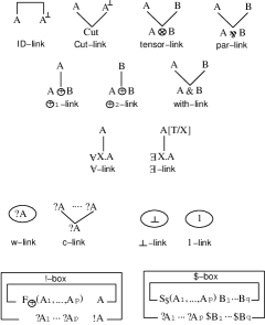
Fig. 1: the links in the LLL system

Figure 2 shows simple proof nets are defined inductively. The formulas and links in simple proof nets have weights. These weights are generated from eigenweights that are associated with $\binampersand$-links occurring in simple proof nets by using boolean product operator ’$\cdot$’. If a formula or a link has the weight $1$, then we omit the weight.

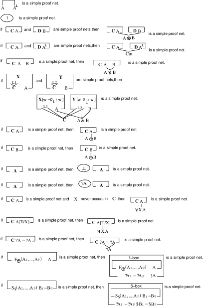
Fig. 2: the definition of simple proof nets

Moreover we must take care of the case of $\binampersand$-links. For example from two simple proof nets of Figure 3 we can construct a simple proof net with the conclusions $?A^{\bot},?B^{\bot},!A\binampersand\$A$ of Figure 4. As shown in the figure, the context-formulas must be shared.

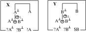
Fig. 3: two simple proof nets

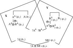
Fig. 4: An example of constructions of simple proof nets with $\binampersand$-links

Moreover sharing of context-formulas may be complex. For example, from two simple proof nets of Figure 5 we can construct a simple proof net with

$$!A\binampersand\$D,?B^{\bot},?C^{\bot},?D^{\bot},\$C\otimes!A.$$

But it is difficult to write down this on a plane in a concise way. So we omit this.

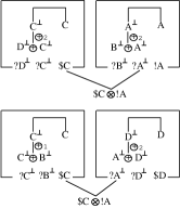
Fig. 5: more two simple proof nets

Figure 6 shows an example that is a proof net in the sense of [Gir96]. The proof net satisfies the correctness condition of [Gir96]. But it is not simple. However we can easily construct a simple proof net that has the same conclusions as the proof net. For example a simple proof net corresponding to that of Figure 6 is that of Figure 7. But such a simple proof net is not uniquely determined. For instance, Figure 8 shows another simple proof net corresponding to that of Figure 6. Besides, in the introduction rules of $!$-box and $\$$-box when we replace $\oplus$-occurrences of generalized $\oplus$-formulas by comma delimiters, we can easily find that any modified simple proof net in this manner is a proof net of Girard by induction on derivations of simple proof nets.

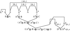
Fig. 6: An example of non-simple proof nets

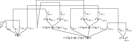
Fig. 7: A simple proof net corresponding to the above non-simple net

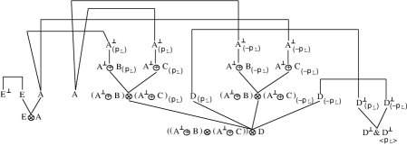
Fig. 8: Another simple proof net corresponding to the above non-simple net

Figure 9 shows the rewrite rules in the LLL system except for contraction, neutral, $!$-$!$, and $!$-$\$$ rewrite rules. Fusion and c-w rewrite rules first appeared in [DK97]. The other rewrite rules in Figure 9 are standard in Linear Logic. Figure 10 shows neutral rewrite rule. Figure 11 shows contraction rewrite rule, where ${\bf\$Y}$, ${\bf\$Y^{\prime}}$, ${\bf!Z}$ and ${\bf!Z^{\prime}}$ represent sequences of proof nets and ’w’ a sequence of weakening links. The length of ${\bf\$Y}$ must be the same as that of ${\bf\$Y^{\prime}}$ and the length of ${\bf!Z}$ the same as that of ${\bf!Z^{\prime}}$. Let ${\bf\$Y}=Y_{1},\ldots,Y_{m}$, ${\bf\$Y^{\prime}}=Y^{\prime}_{1},\ldots,Y^{\prime}_{m}$, ${\bf\$Z}=Z_{1},\ldots,Z_{n}$, ${\bf\$Z^{\prime}}=Z^{\prime}_{1},\ldots,Z^{\prime}_{n}$. Each $Y_{i}\,(1\leq i\leq m)$ and $Z_{\ell}\,(1\leq\ell\leq n)$ must have the following conditions:

1. The conditions on $Z_{\ell}$.
   Each $Z_{\ell}$ must have the form of the upper proof net of Figure 12 or that of Figure 13. In both proof nets, the first $j$ arguments of $G_{\oplus}(A_{1},\ldots,A_{n})$ are all $A^{\bot}$ occurrences and all the links from $A_{i}$ to $G_{\oplus}(A_{1},\ldots,A_{n})$ are $\oplus$-links that have weight $1$ (therefore all the formulas from $A_{i}$ to $G_{\oplus}(A_{1},\ldots,A_{n})$ are not conclusions of two links. We call such a sequence of $\oplus$-links $\oplus$-chain). In the former case $A_{i}$ is equal to $A^{\bot}$ (in this case $i\leq j$) and in the latter case $A_{i}$ not (in this case $i>j$). We call the former $\oplus$-chain non-fake and the latter fake.

2. The conditions on $Y_{i}$.
   Each $Y_{i}$ must have the form of the upper proof net of Figure 14 or that of Figure 15. In the former case there are some non-fake chains, but in the latter case all the $\oplus$-chains are fake.

In other words each proof net in ${\bf\$Y}$ and ${\bf!Z}$ must have at least one $\oplus$-chain. Moreover each $Y^{\prime}_{i}\,(1\leq i\leq m)$ and $Z^{\prime}_{\ell}\,(1\leq\ell\leq n)$ must have the following forms according to $Y_{i}$ and $Z_{\ell}$:

1. The case where the $PLUS$-chain of $Z_{\ell}$ is non-fake:
   Then $Z^{\prime}_{\ell}$ must be the lower proof net of Figure 12.

2. The case where the $\oplus$-chain of $Z_{\ell}$ is fake:
   Then $Z^{\prime}_{\ell}$ must be the lower proof net of Figure 13.

3. The case where some $\oplus$-chains of $Y_{i}$ are non-fake:
   Then $Y^{\prime}_{i}$ must be the lower proof net of Figure 14. The notation $\hat{?B_{r_{j}}}$ of the right side means that the weakening link with conclusion ${?B_{r_{j}}}$ is missing in the proof net.

4. The case where all the $\oplus$-chains of $Y_{i}$ are fake:
   Then $Y^{\prime}_{i}$ must be the lower proof net of Figure 15.

Note that neither the left hand side nor the right hand side of Figure 11 is a simple proof net. If we find a pattern of the left hand side of Figure 11 in a simple proof net, we can apply the contraction rule to the simple proof net and replace the pattern by an appropriate instantiation of the right hand side of Figure 11.

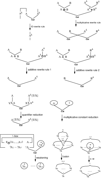
Fig. 9: the rewrite rules in the LLL system

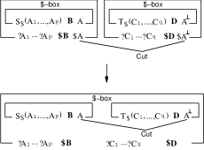
Fig. 10: neutral rewrite rule

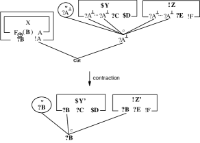
Fig. 11: contraction rewrite rule

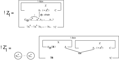
Fig. 12: The case where $Z_{\ell}$ has the non-fake $\oplus$-chain

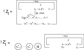
Fig. 13: The case where $Z_{\ell}$ has the fake $\oplus$-chain

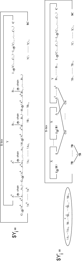
Fig. 14: The case where $Y_{i}$ has non-fake $\oplus$-chains

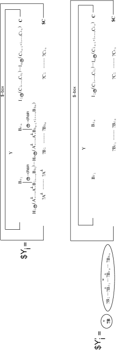
Fig. 15: The case where $Y_{i}$ does not have any non-fake $\oplus$-chains

Let us recall lazy cut elimination in [Gir96].

Definition 1

Let $L$ be a Cut-link in an additive proof net. When two premises of $L$ are $A$ and $A^{\bot}$, $L$ is ready if

1. $L$ has the weight $1$;

2. Both $A$ and $A^{\bot}$ are the conclusion of exactly one link.

For example, in Figure 16, the right cut is ready, but the left not. After the right cut is rewritten, the left become ready.

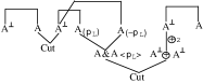
Fig. 16: An example of ready cuts and non-ready cuts

Lazy cut elimination is a reduction procedure in which only ready cuts are redexes (of course, in the contraction rewrite rule the above mentioned conditions must be satisfied). The definition also applies to our rewrite rules. So we use the definition. By $\to_{\mathop{\rm lazy}\nolimits}$ we denote one step reduction of lazy cut elimination.

Theorem 1

Let $\Theta_{1}$ be a simple proof net. If $\Theta_{1}\to_{\mathop{\rm lazy}\nolimits}\Theta_{2}$, then $\Theta_{2}$ is also a simple proof net.

• Induction on the construction of simple proof net $\Theta_{1}$ and an easy argument on permutations of links.    

Next, we relate lazy cut elimination of simple proof nets with that of Girard’s proof nets.

Proposition 1

One step of lazy cut elimination of simple proof nets can be simulated by several steps of that of Girard’s proof nets.

We do not present the proof because in order to prove this we must rephrase the full details of Girard’s proof nets. We just show the difference between them. The left cut of Figure 17 is a redex of Girard’s lazy cut elimination, but not of that of simple proof nets. In Girard’s lazy cut elimination, Figure 17 can be reduced to Figure 18. That does not happen to simple proof nets. Instead of that, in lazy cut elimination of simple proof nets the right cut of Figure 17 is ready and Figure 17 can be reduced to Figure 19. Then the residual left cut of Figure 19 become ready. In lazy cut elimination of simple proof nets, Figure 19 is reduced to Figure 20 by one-step. But in Girard’s lazy cut elimination this reduction takes two-steps. For example we need an intermediate proof net like Figure 21.

It is obvious that there is a proof net that is reduced to a cut-free form in Girard’s lazy cut elimination, but not in lazy cut elimination of simple proof nets. Hence, in this sense, our lazy cut elimination is weaker than that of Girard’s proof nets. But, when we execute Theorem 4, that is, compute polynomial bounded functions on binary integers in proof nets, our lazy cut eliminations and Girard’s always return the same result, since this is due to the following Girard’s theorem and our binary integer encoding in simple proof nets does not have any $\binampersand$-occurrences.

Theorem 2 ([Gir96])

Let $\Theta$ be a proof-net whose conclusions do not contain the connective $\binampersand$ and $\exists X.$ and without ready cut; then $\Theta$ is cut-free.

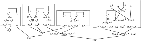
Fig. 17: an example that is a redex of Girard’ proof nets but not that of simple proof nets

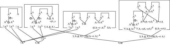
Fig. 18: a contractum of Girard’s proof nets

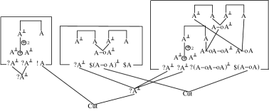
Fig. 19: an example that is a redex of simple proof nets

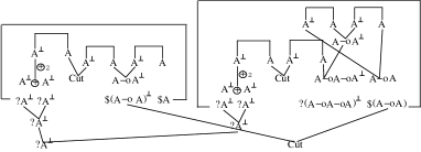
Fig. 20: a contractum of Figure 19

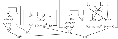
Fig. 21: an intermediate proof net

3 A Turing Machine Encoding

Let $M$ be a Turing machine and $k$ be the number of the states of $M$. Without loss of generality, we can assume that only $0$, $1$, and $\ast$ occur in the tape of $M$, where $\ast$ is the blank symbol of $M$.

We use

$${\bf bool^{k}}\equiv_{\mathop{\rm def}\nolimits}\forall X.\overbrace{X\binampersand(\cdots\binampersand(X\binampersand X)\cdots)}^{k}\mathop{-\circ}X$$

for the type of the states of $M$. In contrast to ${\bf bool^{k}}$ in [Gir98], ${\bf bool^{k}}$ in this paper does not include the neutral connective $\$$. Figure 22 shows an example of ${\bf bool^{k}}$ proofs. After $0$ or $1$ $\oplus_{1}$-link, $\oplus_{2}$-links follow $k-1$ or $i-1$ times.

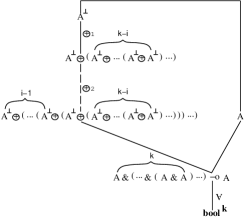
Fig. 22: an example of ${\bf bool^{k}}$ proofs

In addition we use

$${\bf config}\equiv_{\mathop{\rm def}\nolimits}\forall X.!(X\mathop{-\circ}X)\mathop{-\circ}!(X\mathop{-\circ}X)\mathop{-\circ}!(X\mathop{-\circ}X)\mathop{-\circ}\$(X\mathop{-\circ}X\mathop{-\circ}(X\otimes X)\otimes{\bf bool^{k}})$$

for the type of configurations of $M$. The type represents the current configuration of running $M$, that is, the 3-tuple of the left part of the current tape, the right part, and the current state. Figure 23 shows an example of ${\bf config}$ proofs. In the $\lambda$-notation, the example is $\lambda f_{0}.\lambda f_{1}.\lambda f_{\ast}.\lambda x.\lambda y.\langle f_{0}(f_{1}(x)),f_{\ast}(f_{1}(f_{0}(y))),b\rangle$, where $b$ is a ${\bf bool^{k}}$-value. Hence the example denotes configuration $\langle 10,\ast 10,b\rangle$.

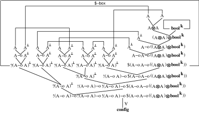
Fig. 23: an example of ${\bf config}$ proofs

For shorthand, we use ${\bf id}_{A}$ to represent $A\mathop{-\circ}A$. Then we write down the transition function of $M$ in Light Linear Logic, which is the main task of the paper. Figure 24 shows our encoding of the transition function, where ${\bf trpl}_{A}$ is an abbreviation of $({\bf bool^{4}}\binampersand 1)\otimes(({\bf id}_{A}\binampersand 1)\otimes A)$. The formula ${\bf trpl}_{A}$ is fed to the second-order variable that is bound by the $\forall$-link in an input proof of ${\bf config}$.

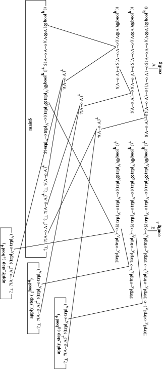
Fig. 24: transition function

Three proof nets apply_step($0^{\bf bool^{4}}$), apply_step($1^{\bf bool^{4}}$), and apply_step($\ast^{\bf bool^{4}}$) in Figure 24 are made up by giving a ${\bf bool^{4}}$ proof ($0$, $1$, or $\ast$) to step of Figure 25 (see Figure 26), where $0^{\bf bool^{4}}$, $1^{\bf bool^{4}}$, and $\ast^{\bf bool^{4}}$ are different normal proof net of ${\bf bool^{4}}$. $0^{\bf bool^{4}}$, $1^{\bf bool^{4}}$, and $\ast^{\bf bool^{4}}$ represent the symbols $0$, $1$, and $\ast$ on the tape of $M$. The main purpose of these apply_step($\Theta^{\bf bool^{4}}$) is to decompose the left or right part of the tape of a given configuration into data with type ${\bf trpl}_{A}=({\bf bool^{4}}\binampersand 1)\otimes(({\bf id}_{A}\binampersand 1)\otimes A)$, where both ${\bf bool^{4}}\binampersand 1$ and ${\bf id}_{A}\binampersand 1$ represent the top symbol of the left or right part of the tape and $A$ represents the rest except for the top symbol. The principle by which the encoding works is the same as that used in writing down the predecessor function. There is just one proof net of ${\bf bool^{4}}$ that are different from these three. Let the proof net be ${\tt empty}^{\bf bool^{4}}$. The proof net ${\tt empty}^{\bf bool^{4}}$ do not have any corresponding symbol on the tape of $M$: the proof net is used in apply_base of Figure 28 in order to make our encoding easy.

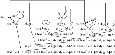
Fig. 25: step function

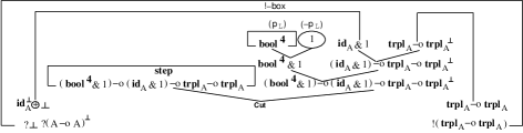
Fig. 26: apply_step

The proof net main$ in the $\$$-box in Figure 24 is shown in Figure 27.

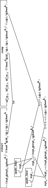
Fig. 27: main$

Proof net apply_base in Figure 27 are made up by giving a ${\bf bool^{4}}$ proof empty to base of Figure 28, where as we mentioned before, ${\tt empty}^{\bf bool^{4}}$ is a normal proof net of ${\bf bool^{4}}$, which is different from $0^{\bf bool^{4}}$, $1^{\bf bool^{4}}$, and $\ast^{\bf bool^{4}}$. The proof net apply_base is used in order to feed an initial value to apply_step($\Theta^{\bf bool^{4}}$).

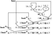
Fig. 28: base function and apply_base

Proof net extract in Figure 27 is shown in Figure 29. The intention of extract was to transform an input of the net $\langle\langle b_{1},\langle f_{1},a_{1}\rangle\rangle,\langle\langle b_{2},\langle f_{2},a_{2}\rangle\rangle,bk\rangle\rangle$ with type $({\bf bool^{4}}\binampersand 1)\otimes(({\bf id}_{A}\binampersand 1)\otimes A)\otimes(({\bf bool^{4}}\binampersand 1)\otimes(({\bf id}_{A}\binampersand 1)\otimes A)\otimes{\bf bool^{k}})$ into $\langle\langle\langle\langle b_{2},f_{1}\rangle,a_{1}\rangle,a_{2}\rangle,bk\rangle$ with type $((({\bf bool^{4}}\otimes{\bf id}_{A})\otimes A)\otimes A)\otimes{\bf bool^{k}}$. The top symbol of the left part of the current tape must be left with type ${\bf id}_{A}$ since this is used in order to be attached to the left or right part of the tape of the next configuration. The top symbol of the right part of the current tape, at which the head of $M$ currently points, must be left with type ${\bf bool^{4}}$ since this is used in order to choose one of select functions (which are defined later). Note that to do this one must use additive connectives and multiplicative constants.

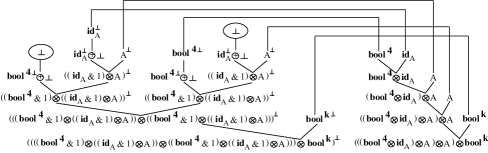
Fig. 29: extract function

Proof net comp in Figure 27 is shown in Figure 30, where

$${\bf shift}\equiv_{\mathop{\rm def}\nolimits}\forall X.(X\mathop{-\circ}X)\mathop{-\circ}X\mathop{-\circ}X\mathop{-\circ}((X\otimes X)\otimes{\bf bool^{k}})$$

and

$${\bf row}\equiv_{\mathop{\rm def}\nolimits}{\bf shift}\binampersand({\bf shift}\binampersand({\bf shift}\binampersand{\bf shift})).$$

The main purpose of extract is to transform an input of the net $\langle\langle\langle\langle b,f\rangle,a_{1}\rangle,a_{2}\rangle,bk\rangle$ with type $((({\bf bool^{4}}\otimes{\bf id}_{A})\otimes A)\otimes A)\otimes{\bf bool^{k}}$ into the next configuration $\langle\langle a_{3},a_{4}\rangle,bk^{\prime}\rangle$ with type $(A\otimes A)\otimes{\bf bool^{k}}$. Data $b$ with type ${\bf bool^{4}}$ and $bk$ with type ${\bf bool^{k}}$ in the input are used in order to choose one of select functions (which are defined later).

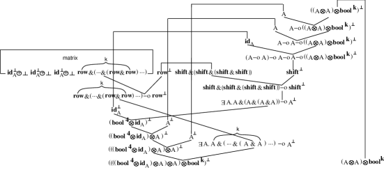
Fig. 30: comp

Proof net matrix in Figure 30 is shown in Figure 33, where $r_{1},\ldots,r_{k-1},r_{k}$ are proof nets that have the form of Figure 34. The main purpose of matrix is to retain $k$ proof nets of the form of Figure 34. Proof nets $s_{1},s_{2},s_{3},$ and $s_{4}$ in Figure 34 have the form of Figure 31 or Figure 32. We call such proof nets shift functions. Proof nets that have the form of Figure 31 represent left moves of the head of $M$. On the other hand proof nets that have the form of Figure 32 represent right moves of the head of $M$.

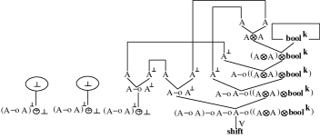
Fig. 31: an example of ${\bf shft}$ proofs (left move)

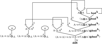
Fig. 32: an example of ${\bf shft}$ proofs (right move)

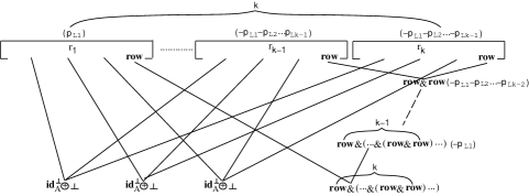
Fig. 33: matrix

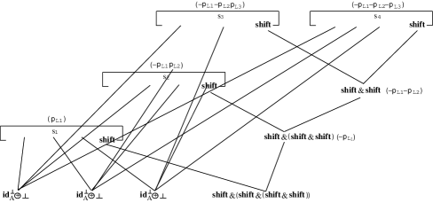
Fig. 34: row_net

From what precedes it is obvious that we can encode the transition function of $M$ into a proof net with conclusions $?\bot,{\bf config}^{\bot},{\bf config}$ of Light Linear Logic. By using the proof net, as shown in Appendix A, P-time Turing machines can be encoded. In other terms, we obtain the following theorem:

Theorem 3

Let ${\bf bint}$ be $\forall X.!(X\mathop{-\circ}X)\mathop{-\circ}!(X\mathop{-\circ}X)\mathop{-\circ}\$(X\mathop{-\circ}X)$. Let $M$ be a Turing machine with time bound of a polynomial with degree $k$. In Light Linear Logic $M$ can be represented by a proof net with conclusions $\bot^{k+4},{\bf bint}^{\bot},\$^{k+3}{\bf config}$.

Furthermore, we can strengthen the above theorem as follows:

Theorem 4

Let $f$ be a polynomial-time function with degree $k$. In Light Linear Logic $f$ can be represented by a proof net with conclusions $\bot^{k+6},{\bf bint}^{\bot},\$^{k+5}{\bf bint}$.

In order to prove the theorem, we need a proof net that transforms ${\bf config}$ into ${\bf bint}$. In Appendix B, we show a proof net that performs the translation.

4 Our Nondeterministic Extension of the Light Linear Logic System

In this section we consider a nondeterministic extension of the LLL system called the NDLLL system. In this extended system we introduce a new self-dual additive connective “nondeterministic with” $\blacktriangle$. Then the formulas of NDLLL are constructed by adding the following clause to that of LLL:

$$F=...|F\blacktriangle F$$

Since $\blacktriangle$ is a self-dual connective, the negation of the formula $A\blacktriangle B$ is defined as follows:

• $(A\blacktriangle B)^{\bot}\equiv_{\mathop{\rm def}\nolimits}A^{\bot}\blacktriangle B^{\bot}$

The link newly introduced in NDLLL is the form of Figure 35. Proof nets for the NDLLL system are inductively defined from the rules of Figure 2 and in the middle of Figure 35. In a simple proof net for NDLLL a unique eigenweight is assigned to each $\blacktriangle$-link occurrence in the same manner as that of $\binampersand$-link.
Finally the rewrite rules of NDLLL are that of LLL plus the nondeterministic rewrite rule of Figure 35. In the rewrite rule for $\blacktriangle$ any of the two contractums is nondeterministically selected. If the left contractum (resp. the right contractum) of Figure 35 is selected, then all the occurrences of both eigenweights for $A\blacktriangle B$ and $A^{\bot}\blacktriangle B^{\bot}$ are assigned to 1 (resp. 0). In the next section we explain a usage for the $\blacktriangle$.

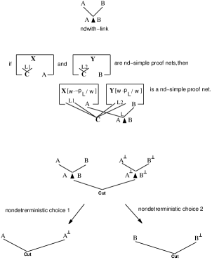
Fig. 35: Our nondeterministic extension of the LLL system

4.1 A Nondeterministic Turing Machine Encoding

Our usage of $\blacktriangle$-connective is to use $\blacktriangle$ in proof nets on datatypes like ${\bf bool}\equiv_{\mathop{\rm def}\nolimits}\forall X.X\binampersand X\mathop{-\circ}X$ which use the standard additive connectives $\binampersand$ and $\oplus$. As an example, we consider cut-elimination of Figure 36, where note that the sub-proof net with conclusion ${\bf bool}\mathop{-\circ}{\bf bool}$ of the right premise of Cut is constructed by using $\blacktriangle$. From Figure 36 to Figure 40 the standard lazy cut elimination procedure is performed. In Figure 40 the nondeterministic cut elimination procedure defined in previous section is performed. Figure 41 is one choice and Figure 42 the other choice.

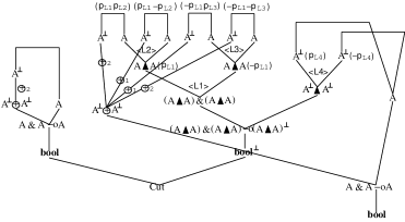
Fig. 36: An example: the starting point

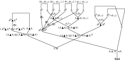
Fig. 37: An example: step 1

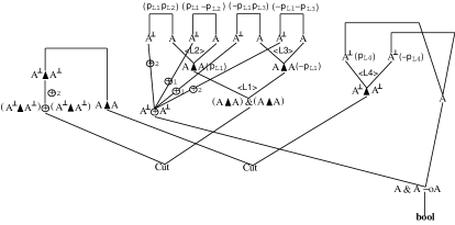
Fig. 38: An example: step 2

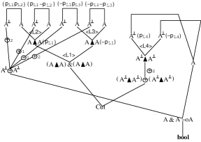
Fig. 39: An example: step 3

Fig. 40: An example: step 4

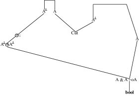
Fig. 41: An example: nondeterministic choice 1

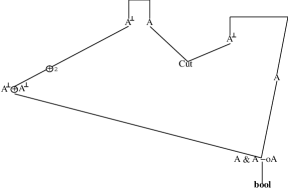
Fig. 42: An example: nondeterministic choice 2

An encoding of a nondeterministic Turing machine into NDLLL uses the same idea. The encoding is the same as that of a deterministic Turing machine into LLL except for comp of Figure 30. The comp proof net is replaced by the nd-comp of Figure 43, where

$${\bf ndrow}\equiv_{\mathop{\rm def}\nolimits}({\bf shift}\blacktriangle{\bf shift})\binampersand(({\bf shift}\blacktriangle{\bf shift})\binampersand(({\bf shift}\blacktriangle{\bf shift})\binampersand({\bf shift}\blacktriangle{\bf shift}))).$$

The idea is completely the same as that of the above example. The information about nondeterministic transitions of a nondeterministic Turing machine is stored in a proof of

$$\overbrace{{\bf ndrow}\binampersand(\cdots\binampersand({\bf ndrow}\binampersand{\bf ndrow}}^{k})\cdots).$$

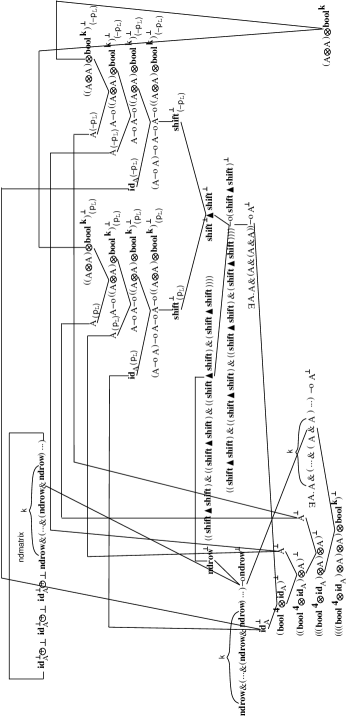
Fig. 43: nd-comp

By the completely same manner as Theorem 3 except for nd-comp the following theorem holds.

Theorem 5

Let $M$ be a nondeterministic Turing machine with time bound of a polynomial with degree $k$. In Nondeterministic Light Linear Logic $M$ can be represented by a proof net with conclusions $\bot^{k+4},{\bf bint}^{\bot},\$^{k+3}{\bf config}$.

Usually a nondeterministic Turing machine characterizes a language accepted by the machine. Without loss of generality, we can assume that nondeterministic Turing machine has two special state symbols ${\tt yes}$ and ${\tt no}$ which judge whether a word is accepted by the machine. Moreover we can prove the following theorem.

Theorem 6

Let $L\subseteq\{0,1\}^{\ast}$ be a language whose is accepted by a nondeterministic polynomial-time Turing machine $M$ with degree $k$. In Nondeterministic Light Linear Logic the characterization function of $L$ from $\{0,1\}$ to $\{0,1\}$ can be represented by a proof net with conclusions $\bot^{k+5},{\bf bint}^{\bot},\$^{k+4}{\bf bool}$.

In order to obtain such a proof net from the proof net with conclusions $\bot^{k+4},{\bf bint}^{\bot},\$^{k+3}{\bf config}$ constructed from Theorem 5, at first we construct a proof net which extracts a ${\bf bool^{k}}$ proof from a ${\bf config}$ proof. Figure 44 shows the proof net. Next we construct a proof net which maps a ${\bf bool^{k}}$ proof to a ${\bf bool}$ proof. The specification of proof net is that

1. if a given ${\bf bool^{k}}$ proof net represents ${\tt yes}$, then the return value is a ${\bf bool}$ proof net that represents ${\tt yes}$;

2. otherwise, the return value is a ${\bf bool}$ proof net that represents ${\tt no}$.

We can easily construct such a proof net.

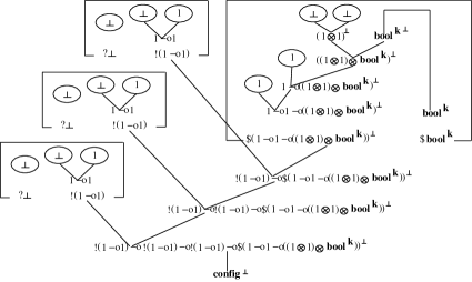
Fig. 44: config2boolk

4.2 Time Bound of Nondeterministic Light Linear Logic

Next we discuss the P-time bound of lazy cut elimination. We define the size of a link to be the number of the conclusions of the link. Moreover we define the size of a nd-simple proof net $\Theta$ (denoted by $\mathop{\rm size}\nolimits(\Theta)$ to be the sum of the sizes of the links in $\Theta$. The depth of $\Theta$ (denoted by $\mathop{\rm depth}\nolimits(\Theta)$) is defined to be the maxmal nesting number of the boxes ($!$-boxes or $\$$-boxes) in $\Theta$. As discussed in [Gir98], $\mathop{\rm size}\nolimits(\Theta)$ is quadratic w.r.t the encoded data generated from $\Theta$. When $\Theta_{1}\to_{\mathop{\rm lazy}\nolimits}\Theta_{2}$ by nondeterministic choice, it is obvious that the size of $\Theta_{2}$ is strictly less than that of $\Theta_{1}$. We suppose that $\Theta\to_{\mathop{\rm lazy}\nolimits}^{\ast}\Theta^{\prime}$, where $\to_{\mathop{\rm lazy}\nolimits}^{\ast}$ is the reflexive transitive closure of $\to_{\mathop{\rm lazy}\nolimits}$. From the above observation and the discussion in [Gir98] on the LLL system, the following proposition is obvious.

Proposition 2

In the NDLLL system, if $\Theta\to_{\mathop{\rm lazy}\nolimits}^{\ast}\Theta^{\prime}$, then the size of $\Theta^{\prime}$ is bounded by $\mathop{\rm size}\nolimits(\Theta)^{2^{\mathop{\rm depth}\nolimits(\Theta)}}$.

It is easy to see that on the above proposition we can lazily reduce $\Theta$ to $\Theta^{\prime}$ in a polynomial time w.r.t $\mathop{\rm size}\nolimits(\Theta)^{2^{\mathop{\rm depth}\nolimits(\Theta)}}$, because $\mathop{\rm size}\nolimits(\Theta)$ is quadratic w.r.t the encoded data generated from $\Theta$.

Proposition 3

In the NDLLL system, if $\Theta\to_{\mathop{\rm lazy}\nolimits}^{\ast}\Theta^{\prime}$, then $\Theta$ is reduced to $\Theta^{\prime}$ in a polynomial time w.r.t $\mathop{\rm size}\nolimits(\Theta)^{2^{\mathop{\rm depth}\nolimits(\Theta)}}$.

Let $M$ be a nondeterministic polynomial-time Turing machine with degree $k$. Then by Theorem 5 we can construct a nd-simple proof net $\Theta_{1}$ with conclusions $\bot^{k+4},{\bf bint}^{\bot},\$^{k+3}{\bf config}$. Then let $\Theta_{2}$ be a simple proof net with the conclusion ${\bf bint}$ representing a binary integer with length $n$. Then from Proposition 3 we can see the proof net constructed by connecting $\Theta_{1}$ and $\Theta_{2}$ via Cut-link is lazily and nondeterministically reduced to a normal form in a polynomial time w.r.t $n^{2^{k}}$.

5 Concluding Remarks

It seems possible that a P-time Turing machine encoding in Light Affine Logic is mechanically translated into that in Light Linear Logic. A given proof of the P-time Turing machine encoding in Light Affine Logic, we replace all the formula occurrences $A$ in the proof by $A\binampersand 1$ and then apply an extract function like Figure 29 to the resulting proof. But we did not adopt the method, since the simple transition makes a too redundant proof in Light Linear Logic. So we made some optimizations. For example, In [Rov99] $\forall X.X\otimes X\mathop{-\circ}X$ was used as the boolean type. The above mentioned translation makes $\forall X.((((X\binampersand 1)\otimes(X\binampersand 1))\binampersand 1)\mathop{-\circ}(X\binampersand 1))\binampersand 1$. The study to find optimal translations seems interesting.

Acknowledgements.    The author thanks Luca Roversi for discussions at his visit to University of Torino.

A Our encoding of Turing machines(continued)

For shorthand, we use $!^{k}A$ to represent $\overbrace{!(\cdots!(!}^{k}A)\cdots)$. We also use $?^{k}A\equiv_{\mathop{\rm def}\nolimits}\overbrace{?(\cdots?(?}^{k}A)\cdots)$ and $\$^{k}A\equiv_{\mathop{\rm def}\nolimits}\overbrace{\$(\cdots\$(\$}^{k}A)\cdots)$ In addition, we implicitly assume coercion for $\bot$. In other terms, we assume that by using a proof net with conclusions $?^{k_{1}}\bot,\ldots,?^{k_{p}}\bot,\Gamma$ we can construct a proof net with conclusions $?^{k}\bot,\Gamma$ provided $k\geq k_{1},\ldots,k_{p}$. This is done by using $p$ proof nets that have the forms of Figure 45, Cut-links, and one contraction-link.

Fig. 45: coercion of $\bot$

Unlike [Gir98], we do not use ${\bf int}\equiv_{\mathop{\rm def}\nolimits}\forall X.!(X\mathop{-\circ}X)\mathop{-\circ}\$(X\mathop{-\circ}X)$ for our Turing machine encoding: we only use ${\bf bint}\equiv_{\mathop{\rm def}\nolimits}\forall X.!(X\mathop{-\circ}X)\mathop{-\circ}!(X\mathop{-\circ}X)\mathop{-\circ}\$(X\mathop{-\circ}X)$ instead of ${\bf int}$ since we would like to reduce the number of proof nets appearing in this paper. It is possible to construct a Turing machine encoding from our transition function encoding by using ${\bf int}$. In the following we show three basic functions for ${\bf bint}$: two successor function and addition. Figure 46 and Figure 47 show two successor functions for ${\bf bint}$: we call these suc0 and suc1 respectively. Unlike ${\bf int}$, ${\bf bint}$ has two successor functions.

Fig. 46: suc0

Fig. 47: suc1

Figure 48 shows the analogue in ${\bf bint}$ to the addition in ${\bf int}$: we call the proof net badd. If we regard two inputs proofs of ${\bf bint}$ of the proof net as two lists which only have $0$ and $1$, then we can regard badd as a concatenation function of two inputs.

Fig. 48: badd

Figure 49 shows a proof net called bmul. In the figure, empty is a proof net of ${\bf bint}$ that does not have exponential-links except for two weakening-links with $?(A\mathop{-\circ}A)^{\bot}$. Let $\Theta_{1}$ be a ${\bf bint}$ proof that is supplied to ${\bf bint}^{\bot}$ port of bmul and $\Theta_{2}$ be a proof net with $!{\bf bint}$ as one of conclusions that is supplied to $?{\bf bint}^{\bot}$ port of bmul. Let $\ell$ be the length of $\Theta_{1}$. The evaluated result of bmul provided inputs $\Theta_{1}$ and $\Theta_{2}$ are given, is $\ell$ copies of $\Theta_{2}$. Let $m$ be the length of $\Theta_{2}$. The length of the result is $\ell\times m$. The proof net bmul is analogous to multiplication of ${\bf int}$.

Fig. 49: bmul

The proof net shown in Figure 50 transform a ${\bf bint}$ proof into a ${\bf config}$ proof that is a initial configuration of Turing machines. We call the proof net bint2config. By using bint2config and transition, our encoding of the transition function of $M$, we can construct the engine part of Turing machines shown in Figure 51. But it is not sufficient for a proof of Theorem 3: besides we need constructions for polynomial time bound. To do this, we prepare several proof nets.

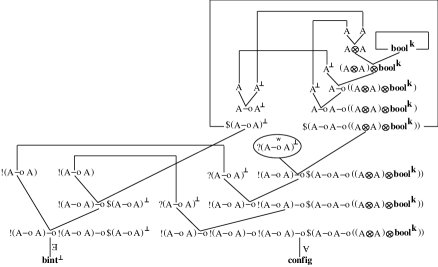
Fig. 50: bint2config

Fig. 51: tm_engine

The proof net ${\tt coer}^{p,q}$ of Figure 52 is the ${\bf bint}$ version of ${\bf int}$ coercion of [Gir98]. Then $p$ must be greater than $0$. This proof net is used in Figure 54 and Figure 56.

Fig. 52: ${\tt coer}^{p,q}$

The proof net k-contraction of Figure 53 is also the ${\bf bint}$ version of ${\bf int}$ contraction of [Gir98]. This proof net is used in Figure 54 and Figure 55.

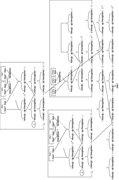
Fig. 53: k-contraction

The proof net in Figure 54 is used in Figure 55. This is basically $k$ compositions of bmul. The ${\bf bint}$ proof $c_{\mathop{\rm const}\nolimits}$ in Figure 54 is a constant that does not depend on the lengths of inputs of Turing machine $M$.

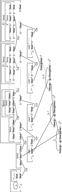
Fig. 54: k-composition of multiplications

The proof net kpolynomial of Figure 55 is our polynomial construction with degree $k$. Let $\Theta$ be a proof net of ${\bf bint}$ and $\ell$ be the length of $\Theta$. The evaluated result of kpolynomial provided an input $\Theta$ is given, is a nest of $\$$-boxes which has an inside proof net of ${\bf bint}$ with the length $c_{\mathop{\rm const}\nolimits}\times\ell^{k}$.

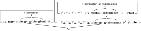
Fig. 55: kpolynomial

Finally we obtain our encoding of a Turing machine with polynomial time bound of Figure 56. This completes our proof of Theorem 3.

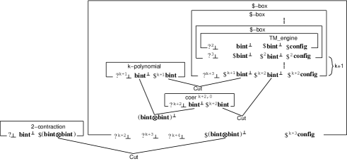
Fig. 56: TM

B A transformation from config proofs into bint proofs

At first we remark that when a given proof net with conclusion $\Gamma$, we can construct a proof net with ${\bf bool^{2}}^{\bot},\Gamma$ as shown in Figure 57. It is easy to extend the remark to the general ${\bf bool^{k}}$ case for $k\leq 2$.
Then based on the above remark, as a derived rule, we introduce ${\bf bool^{k}}$-axiom as shown in Figure 58 in order to keep figures as simple as possible.

Fig. 57: ${\bf bool^{2}}$-weakening

Fig. 58: ${\bf bool^{k}}$-axiom

In order to translate config proofs into bint proofs, we introduce an immediate type ${\bf tint}\equiv_{\mathop{\rm def}\nolimits}\forall X.!(X\mathop{-\circ}X)\mathop{-\circ}!(X\mathop{-\circ}X)\mathop{-\circ}!(X\mathop{-\circ}X)\mathop{-\circ}\$(X\mathop{-\circ}X)$.
Figure 59 shows our translator from config proofs into bint proofs. When a given config proof, at first we duplicate the proof by using 2-contraction-config proof net. A construction of 2-contraction-config proof net is not so easy as that of 2-contraction for bint. Appendix C is devoted to the construction.

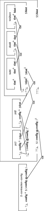
Fig. 59: config2bint

After that, each duplicated config proof net is projected into a tint proof by using prj1 or prj2 shown in Figure 60. The purpose of prj1 is to extract the left parts of configurations of Turing machines and similarly that of prj2 is to extract the right parts.
Proof net prj1 has proof net prj1sub shown in Figure 61 as a sub-proof net and prj2 has prj2sub shown in Figure 62. Proof net prj1 also has proof nets ${\tt tsuc0^{r}}$, ${\tt tsuc1^{r}}$, and ${\tt tsuc*^{r}}$ as sub-proof nets and prj2 has tsuc0, tsuc1, and tsuc*. Figure 63 and Figure 64 show proof net tsuc0 and ${\tt tsuc0^{r}}$ respectively. We omit tsuc1, tsuc*, ${\tt tsuc1^{r}}$, and ${\tt tsuc*^{r}}$, since the constructions of these proof nets are easy exercise. Note that in order to recover tapes correctly we need to reverse the left parts of tapes. Next we concatenate obtained two tint proofs by tadd of Figure 65.

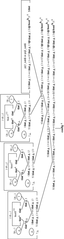
Fig. 60: prj1 or prj2

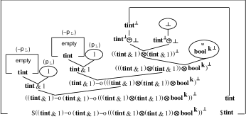
Fig. 61: prj1sub

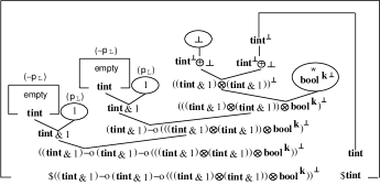
Fig. 62: prj2sub

Fig. 63: tsuc0

Fig. 64: ${\tt tsuc0^{r}}$

Fig. 65: tadd

We distinguish the two normal proofs of ${\bf bool^{2}}$. One is called ${\tt Pi_{01}}$. and the other ${\tt Pi_{\ast}}$ (see Figure 66). Next we apply distill of Figure 67 to the obtained tint proof. The construction of the proof net distill is inspired by that of strip term in [MO00]. The intention of the distill proof net is to keep occurrences of $0$ and $1$ until the first $\ast$ occurrence is reached. After that, the rest are discarded. Figure 68 shows three sub-proof nets distill_step_X (X=1,2, and $\ast$) of the distill proof net. Moreover, two sub-proof nets ${\tt distill\_step\_sub\_X_{L}}$ and ${\tt distill\_step\_sub\_X_{R}}$ of ${\tt distill\_step\_X}$ have the forms of Figure 69 or Figure 70. Table 1 shows the correspondence.
Figure 71 shows tint2bint proof. The intention is to remove $\ast$-entry.

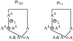
Fig. 66: ${\tt Pi_{01}}$ and ${\tt Pi_{\ast}}$

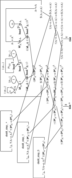
Fig. 67: distill

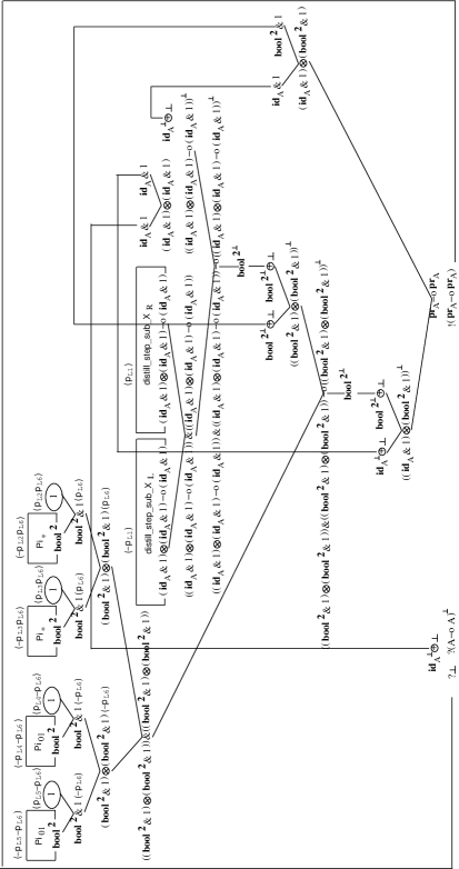
Fig. 68: distill_step_X

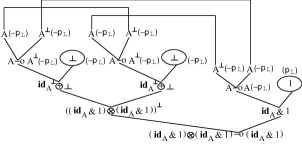
Fig. 69: distill_step_sub_join

Fig. 70: distill_step_sub_discard

	D=L	D=R
X=0	distill_step_sub_join	distill_step_sub_discard
X=1	distill_step_sub_join	distill_step_sub_discard
X=$\ast$	distill_step_sub_discard	distill_step_sub_discard

Table 1: ${\tt distill\_step\_sub\_X_{D}}$

Fig. 71: tint2bint

C Contraction on config

In this section we give how to construct 2-contraction-config proof net. In config2bint of Appendix B we do not need the ${\bf book^{k}}$-part of a given config proof. Hence in the construction of 2-contraction-config proof net we could discard ${\bf book^{k}}$-parts. But we give a general construction that duplicates ${\bf book^{k}}$-parts here. Figure 72 shows 2-contraction-config proof net. In this proof net,

1. when given a config proof net, pre_config_dup of Figure 73 outputs a quartet of config proof nets, where two config proofs are the same and only keep the left part and ${\bf book^{k}}$ of the input, and the rest, which are two config proofs, are also the same and only keep the right part and ${\bf book^{k}}$ of the input;

2. each configadd of Figure 80 concatenate two config proof nets in the quartet.

Type ${\bf dconfig_{2}^{k}}$ of proof net pre_config_dup is defined as follows:

$${\bf config_{2}^{k}}\equiv_{\mathop{\rm def}\nolimits}\overbrace{({\bf config}\otimes{\bf config})\binampersand(\cdots\binampersand(({\bf config}\otimes{\bf config})\binampersand({\bf config}\otimes{\bf config}))\cdots)}^{k}$$

$${\bf dconfig_{2}^{k}}\equiv_{\mathop{\rm def}\nolimits}{\bf config_{2}^{k}}\oplus{\bf config_{2}^{k}}$$

In pre_config_dup, at first, we make $4k$ config proofs. Then according to the ${\bf book^{k}}$-value of the input ${\bf config}$ proof, we choose 4 config proofs. That is why we use $k$-ary tuples by $\binampersand$-connectives in ${\bf config_{2}^{k}}$. In addition we need to distinguish the left part and the right part of the input ${\bf config}$ proof. That is why we use one $\oplus$-connective in ${\bf dconfig_{2}^{k}}$.
Figure 74 shows sub-proof net pre_config_dup_main of pre_config_dup. Note that as shown in Figure 75, we can duplicate ${\bf book^{2}}$ proof without using $\$$ (of course we can easily extend this construction to the ${\bf bool^{k}}$ case).
Proof nets ${\tt dconfig\_sucX}$ (where $X=1,2,\,$ and $\,\ast$) shown in Figure 77 occur in
pre_config_dup_main as sub-proof nets. Figure 78 and Figure 79 show proof nets suc0L and suc0R. We omit suc1L, suc1R, suc$\ast$L and suc$\ast$R since the constructions of these proof nets are easy exercise.

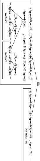
Fig. 72: 2-contraction-config

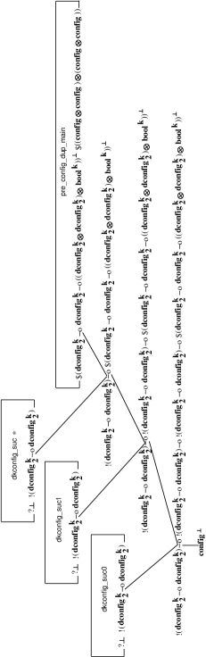
Fig. 73: pre_config_dup

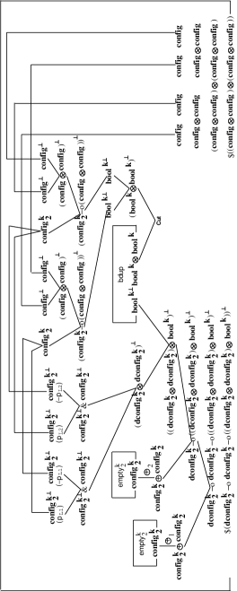
Fig. 74: pre_config_dup_main

Fig. 75: bdup

Fig. 76: ${\tt empty}^{k}_{2}$

Fig. 77: ${\tt dconfig\_sucX}$

Fig. 78: suc0L

Fig. 79: suc0R

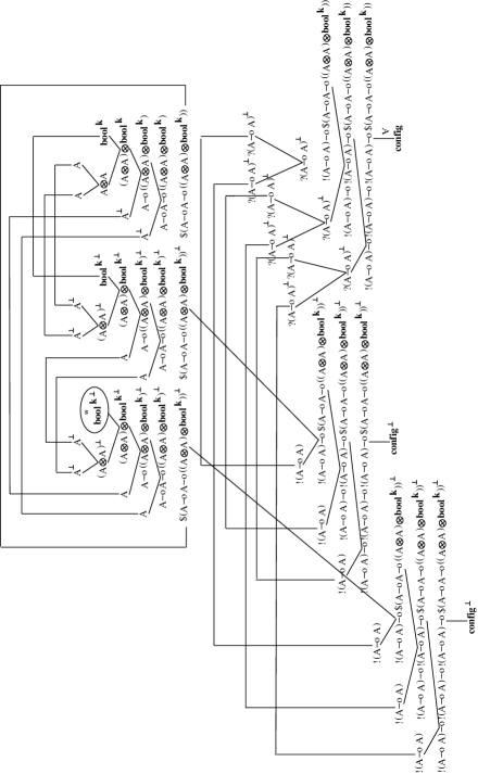
Fig. 80: configadd

Received 07/10/2003

Bibliography

- [AR02] Asperti, A. and Roversi, L. Intuitionistic Light Affine Logic. ACM Transactions on Computational Logic, 3 (1),1–39, 2002.
- [Asp98] Asperti, A. Light Affine Logic. In LICS’98, 1998.
- [DK97] Di Cosmo, R. and Kesner, D. Strong Normalization of Explicit Substitutions via Cut Elimination in Proof Nets. In LICS’97, 1997.
- [Gir87] Girard, J.-Y. Linear logic. Theoretical Computer Science, 50,1–102, 1987.
- [Gir95] Girard, J.-Y. Linear logic: its syntax and semantics. Advances in Linear Logic, London Mathematical Society Lecture Notes Series 222, 1995.
- [Gir96] Girard, J.-Y. (1996) Proof-nets: the parallel syntax for proof-theory. In Ursini and Agliano, editors, Logic and Algebra, New York, Marcel Dekker, 1996.
- [Gir98] Girard, J.-Y. Light Linear Logic. Information and Computation, 143, 175–204, 1998.
- [Mat96] Matsuoka, S. Nondeterministic Linear Logic. IPSJ SIGNotes PROgramming No.12, 1996.
- [MO00] Murawski, A. S. and Ong, C.-H. L. Can safe recursion be interpreted in light logic?. Available from Luke Ong’s home page (http://web.comlab.ox.ac.uk/oucl/work/luke.ong/), 2000.
- [Mau03] Maurel, F. Nondeterministic Light Logics and NP-Time. TLCA 2003, LNCS 2701, 2003.
- [Pap94] Papadimitriou, C. Computational Complexity, Addison Wesley, 1994.
- [Rov99] Roversi, L. A P-Time Completeness proof for light logics. In Ninth Annual Conference of the EACSL (CSL’99), Lecture Notes in Computer Science, 1683, 469–483, 1999.