Weak Typed Böhm Theorem on IMLL

Abstract

In the Böhm theorem workshop on Crete island, Zoran Petric called Statman’s “Typical Ambiguity theorem” typed Böhm theorem. Moreover, he gave a new proof of the theorem based on set-theoretical models of the simply typed lambda calculus.
In this paper, we study the linear version of the typed Böhm theorem on a fragment of Intuitionistic Linear Logic. We show that in the multiplicative fragment of intuitionistic linear logic without the multiplicative unit ${\bf 1}$ (for short IMLL) weak typed Böhm theorem holds. The system IMLL exactly corresponds to the linear lambda calculus without exponentials, additives and logical constants. The system IMLL also exactly corresponds to the free symmetric monoidal closed category without the unit object. As far as we know, our separation result is the first one with regard to these systems in a purely syntactical manner.

1 Introduction

In [DP01], Dosen and Petric called Statman’s “Typical Ambiguity theorem” [Sta83] typed Böhm theorem. Moreover, they gave a new proof of the theorem based on set-theoretical models of the simply typed lambda calculus.
In this paper, we study the linear version of the typed Böhm theorem on intuitionistic multiplicative Linear Logic without the multiplicative unit ${\bf 1}$ (for short IMLL). We consider the typed version of the following statement:

There are two different closed $\beta\eta$-normal terms $\underline{0}$ and $\underline{1}$ such that if $s$ and $t$ are closed untyped normal $\lambda$-terms, and $s\neq_{\beta\eta}t$ then, there is a context $C[]$ such that

$$C[s]=_{\beta\eta}\underline{0}\,\,\,\mbox{ and }\,\,\,C[t]=_{\beta\eta}\underline{1}$$

We call the statement weak untyped Böhm theorem. In this paper, we show that the typed version of weak Böhm theorem holds in IMLL.
The theorem is nontrivial because the system IMLL is rather weak in expressibility. Hence, a careful analysis on IMLL proof nets is needed. The system IMLL exactly corresponds to the linear lambda calculus without exponentials, additives and logical constants. A version of the linear lambda calculus can be found in [MO03]. The system IMLL also exactly corresponds to the free symmetric monoidal closed category without the unit object(see [MO03]). As far as we know, the result we prove in this paper is the first one with regard to these systems in a purely syntactical manner.
On the other hand, we call the following statement strong untyped Böhm theorem:

For any untyped $\lambda$-terms $a$ and $b$, if $s$ and $t$ are closed untyped normal $\lambda$-terms, and $s\neq_{\beta\eta}t$ then, there is a context $C[]$ such that

$$C[s]=_{\beta\eta}a\,\,\,\mbox{ and }\,\,\,C[t]=_{\beta\eta}b$$

We could not prove the typed version of the statement in the system IMLL. But so far we proved the typed version of the statement w.r.t a very limited fragment including additive connectives of Linear Logic (see Section 7). Also note that the weak statement and the strong statement are trivially equivalent in the untyped $\lambda K$-calculus (i.e., the usual $\lambda$-calculus) and in the simply typed $\lambda$-calculus (if type instantiation is allowed) because both systems allow unrestricted weakening.
Although currently we have not developed applications of the theorem, Statman’s typical ambiguity theorem has several applications in foundations of programming languages (for example [SP00]). Intuitionistic Linear Logic has become more important because game semantics is successful as a method giving fully abstract semantics for many programming languages and Intuitionistic Linear Logic can be seen as a foundation for game semantics. We hope that our result contributes to further analysis of proofs and further applications on Linear Logic.
Related works  Our work is obviously based on that of [Sta83] (see also
[Sta80, Sta82, SD92]). As we said before, however, our result can not be derived directly from that of [Sta83], mainly because of lack of unrestricted weakening in IMLL. It is also interesting that unlike ours, the separability result of [Sta83] cannot be obtained simply by substituting a type which has only two closed normal terms: a type which should be instantiated depends on the maximal number of occurrences of variables if you want to restrict the type to have only a finite number of closed terms, since the simply typed lambda calculus allows unrestricted contraction. Of course, you can choose a type which has infinitely many closed terms like the Church integer. But IMLL does not have such a type.
On the other hand, recently, some works [DP00, Jol00, TdF00, TdF03, LT04] other than [DP01] have been also done on similar topics to typed Böhm theorem. However, the system with which [Jol00] and [DP00, DP01] dealt is the simply typed lambda calculus or the free cartesian closed category, not IMLL. The works of [TdF00, TdF03, LT04] are technically completely different from ours.
The structure of the paper  Section 2 and 3 give a definition of IMLL proof nets and an equality on them. Section 4 and 5 give a proof of weak typed Böhm theorem on the implicational fragment of IMLL (for short IIMLL). Section 6 describes a reduction of an unequation of IMLL proof nets to that of IIMLL proof nets. By the reduction we complete a proof of weak typed Böhm theorem on IMLL. Section 7 discusses extensions of our result to IMLL with the multiplicative constant 1, MLL, and IMLL with additives.

2 The IMLL systems

In this section, we present intuitionistic multiplicative proof nets. We also call these IMLL proof nets.

Definition 1

(MLL formulas) MLL formulas (or simply formulas) (F) is inductively constructed from atomic formulas (P) and logical connectives:

• $P=p$

• $F=P\,|\,F\otimes F\,|\,F\bindnasrepma F$.

In this paper, we only consider MLL formulas with the only one propositional variable $p$. All the results in this paper can be easily extended to the general case with denumerable propositional variables, since we just substitute $p$ for these propositional variables.

Definition 2

(IMLL formulas) An IMLL formula is a pair $\langle A,pl\rangle$ where A is an MLL formula and pl is an element of $\{+,-\}$, where $+$ and $-$ are called Danos-Regnier polarities. A formula $\langle A,pl\rangle$ is written as $A^{pl}$. A formula with $+$ (resp. $-$) polarity is called $+$-formula or positive formula (resp. $-$-formula or negative formula).

Figure 1 shows the links we use in this paper. In Figure 1,

1. In ID-link, $A^{+}$ and $A^{-}$ are called conclusions of the link.

2. In Cut-link, $A^{+}$ and $A^{-}$ are called premises of the link.

3. In $\otimes^{-}$-link (resp. $\bindnasrepma^{+}$-link) $A^{+}$ (resp. $A^{-}$) is called the left premise, $B^{-}$ (resp. $B^{+}$) the right premise and ${A\otimes B}^{-}$ (resp. ${A\bindnasrepma B}^{+}$) the conclusion of the link.

4. In $\otimes^{+}$-link (respectively $\bindnasrepma^{-}$-link), $A^{+}$ (resp. $A^{-}$) is called the left premise, $B^{+}$ (resp. $B^{-}$) the right premise and ${A\otimes B}^{+}$ (resp. ${A\bindnasrepma B}^{-}$) the conclusion of the link.

Figure 1: the links we use in this paper

Figure 2 shows that IMLL proof nets are defined inductively, where ${\bf C}^{-}$ and ${\bf D}^{-}$ are a list of $-$-formulas. If $\Theta$ is an IMLL proof net and $\Theta$ is defined without using clauses (4) and (6), then we say that $\Theta$ is an IIMLL proof net. In the definition of IMLL proof nets, we permit ’crossings’ of links, because the IMLL system has an exchange rule. A typical example of such a crossing is that of Figure 20. In an IMLL proof net $\Theta$, a formula occurrence $A$ is a conclusion of $\Theta$ if $A$ is not a premise of a link.

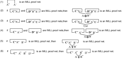
Figure 2: the definition of IMLL proof nets

Next we give the graph-theoretic characterization of IMLL proof nets, following [Gir96], because we use this in the proof of Lemma 3. The characterization was firstly proved in [Gir87] and an improvement was given in [DR89]. First we define IMLL proof structures. Figure 3 shows that IMLL proof structures are defined inductively, where C and D are a list whose element is a $-$-formula or a $+$-formula. Note that the rules from (1) to (6) can be regarded to be generalized ones of that of IMLL proof nets. So, the set of the IMLL proof nets is a subset of the set of the IMLL proof structures. For example, Figure 4 shows two examples of typical IMLL proof structures that are not IMLL proof nets.
In order to characterize IMLL proof nets among IMLL proof structures, we introduce Danos-Regnier graphs. Let $\Theta$ be an IMLL proof structure. We assume that we are given a function $S$ from the set of the occurrences of $\bindnasrepma$-links in $\Theta$ to $\{0,1\}$. Such a function is called a switching function for $\Theta$. Then the Danos-Regnier graph $\Theta_{S}$ for $\Theta$ and $S$ is a undirected graph such that

1. the nodes are all the formula occurrences in $\Theta$, and

2. the edges are generated by the rules of Figure 5.

Theorem 1 ([Gir87] and [DR89])

An IMLL proof structure $\Theta$ is an IMLL proof net iff for each switching function $S$ for $\Theta$, the Danos-Regnier graph $\Theta_{S}$ is acyclic and connected.

A meaning of the theorem is that even though we obtain an IMLL proof structure from an illegal derivation as a derivation of IMLL proof nets, if the proof structure satisfies the criterion of the theorem, then we obtain a legal derivation of IMLL proof nets for the IMLL proof structure, i.e., the IMLL proof structure is an IMLL proof net. Figure 6 shows the situation: the left derivation of Figure 6 is an illegal derivation of IMLL proof nets. But since the derived IMLL proof structure satisfies the criterion of the theorem, the IMLL proof structure is an IMLL proof net and we obtain the right derivation of Figure 6 for the IMLL proof net.

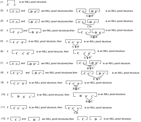
Figure 3: the definition of IMLL proof structures

Figure 4: two examples of IMLL proof structures

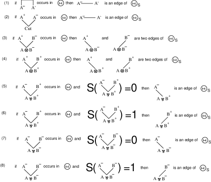
Figure 5: the rules for the generation of the edges of a Danos-Regnier graph $\Theta_{S}$

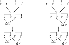
Figure 6: an illegal derivation and a legal derivation of the same IMLL proof net

Next we define reduction on IMLL proof nets. Figure 7 shows the rewrite rules we use in this paper. The ID and multiplicative rewrite rules are usual ones. The multiplicative $\eta$-expansion is the usual $\eta$-expansion in Linear Logic. We denote the reduction relation defined by these five rewrite rules by $\to^{\ast}$. The one step reduction of $\to^{\ast}$ is denoted by $\to$. In the following subsection we show that strong normalizability and confluence w.r.t $\to$ holds. Hence without mention, we identify an IMLL proof net with the normalized net.

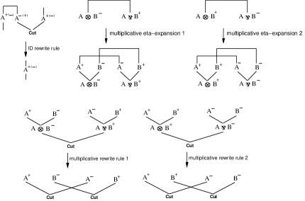
Figure 7: the rewrite rules we use in this paper

Abbreviations

In the following we use an abbreviation using linear implication $\mathop{-\circ}$ instead of $\bindnasrepma$ in order to relate our IMLL formulas to usual IMLL formulas in the linear lambda calculus (for example, in [MO03]).

1. $\mathop{\rm abb}\nolimits(A^{+})={\mathop{\rm sabb}\nolimits(A^{+})}^{+}$     $\mathop{\rm abb}\nolimits(A^{-})={\mathop{\rm sabb}\nolimits(A^{-})}^{-}$

2. $\mathop{\rm sabb}\nolimits({p}^{-})=\mathop{\rm sabb}\nolimits({p}^{+})=p$

3. $\mathop{\rm sabb}\nolimits({A\otimes B}^{-})=\mathop{\rm sabb}\nolimits(A^{+})\mathop{-\circ}\mathop{\rm sabb}\nolimits(B^{-})$     $\mathop{\rm sabb}\nolimits({A\bindnasrepma B}^{+})=\mathop{\rm sabb}\nolimits(A^{-})\mathop{-\circ}\mathop{\rm sabb}\nolimits(B^{+})$

4. $\mathop{\rm sabb}\nolimits({A\otimes B}^{+})=\mathop{\rm sabb}\nolimits(A^{+})\otimes\mathop{\rm sabb}\nolimits(B^{+})$     $\mathop{\rm sabb}\nolimits({A\bindnasrepma B}^{-})=\mathop{\rm sabb}\nolimits(A^{-})\otimes\mathop{\rm sabb}\nolimits(B^{-})$

For example, $\mathop{\rm abb}\nolimits({p\bindnasrepma(((p\otimes p)\bindnasrepma(p\otimes p))\bindnasrepma p)}^{+})$ is ${p\mathop{-\circ}(((p\mathop{-\circ}p)\otimes(p\mathop{-\circ}p))\mathop{-\circ}p)}^{+}$. We identify an IMLL formula $A^{\epsilon}$ with $\mathop{\rm abb}\nolimits(A^{\epsilon})$, where $\epsilon=+$ or $-$. The notation is confusing a little bit: for example, $\mathop{\rm abb}\nolimits({p\bindnasrepma p}^{-})={p\otimes p}^{-}$. This is due to the mismatch between the proof-nets notation and the linear lambda calculus notation. However, from surrounding contexts, i.e., from whether $\bindnasrepma$ or $\mathop{-\circ}$ is used, we can easily judge which notation is adopted.

2.1 Strong normalizability and confluence on the IMLL system

We believe that these two theorems are folklore. We just give the following proofs by a request for an anonymous referee. The strong normalizability is almost trivial. The confluence on IMLL is more complicated because in the IMLL with the multiplicative $\eta$-expansion one-step confluence does not hold unlike the IMLL without the rewrite rule. But we do not think that the proofs that we give here are difficult to understand. If you have no doubt about the strong normalizability and confluence on the IMLL system, you can skip this subsection.

Definition 3 (the SN size of an ID-link and the SN size of a Cut-link)

The SN size of an ID-link is the size of a conclusion, that is, the number of the occurrences of logical connectives in the premise. Note that the choice between a conclusion and the other conclusion is indifferent. Also note that the SN size of an ID-link with two atomic formulas as the conclusions is 0. The SN size of a Cut-link is the size of a premise plus 1. With regard to the SN size of a Cut link, the same remark about the choice between a premise and the other premise as that of an ID-link is also applied. Also note that the SN size of a Cut-link with two atomic formulas as the premises is 1.

Definition 4 (the SN size of an IMLL proof net)

The SN size of an IMLL proof net $\Theta$ is the sum of the SN sizes of all the occurrences of Cut-links and ID-links in $\Theta$.

Proposition 1 (Strong normalizability on the IMLL system)

Let $\Theta$ be an IMLL proof net. $\Theta$ is strong normalizing.

Proof.    Let $\Theta\to\Theta^{\prime}$. Then in any case where $\Theta$ reduces to $\Theta^{\prime}$ by a rule in Figure 7, we can easily see the SN size of $\Theta^{\prime}$ is less than that of $\Theta$. $\Box$

For example, the SN size of $\Theta_{1}$ in Figure 8 is 9. Then $\Theta_{1}\to\Theta_{2}$ by the ID rewrite rule, where $\Theta_{2}$ is the IMLL proof net of Figure 9. The SN size of $\Theta_{2}$ is 0. On the other hand $\Theta_{1}\to\Theta_{3}$ by the multiplicative $\eta$-expansion 1, where $\Theta_{3}$ is the IMLL proof net of Figure 10. The SN size of $\Theta_{3}$ is 8.

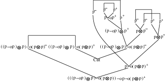
Figure 8: an example of IMLL proof nets with Cut-links $\Theta_{1}$

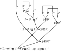
Figure 9: the IMLL proof net $\Theta_{2}$ obtained from $\Theta_{1}$ by the ID rewrite rule

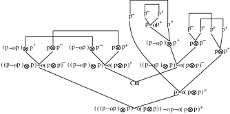
Figure 10: the IMLL proof net $\Theta_{3}$ obtained from $\Theta_{1}$ by the multiplicative $\eta$-expansion 1

Next, we consider the confluence on the IMLL system.
Figure 8, Figure 9, and Figure 10 show a counterexample of one-step confluence in the IMLL system with the multiplicative $\eta$-expansion, since $\Theta_{3}$ of Figure 10 can not reach $\Theta_{2}$ of Figure 9 exactly by one-step. Nevertheless, applying the multiplicative $\eta$-expansion three times to $\Theta_{3}$, we can obtain $\Theta_{4}$ and applying the multiplicative rewrite rule four times and the ID rewrite rule on atomic formulas five times to $\Theta_{4}$ of Figure 11, we can obtain $\Theta_{2}$.
We also give another example. Figure 12, Figure 13, and Figure 14 also show a counterexample of one-step confluence in the IMLL system with the multiplicative $\eta$-expansion, since $\Theta^{\prime}_{3}$ of Figure 14 can not reach $\Theta^{\prime}_{2}$ of Figure 13 exactly by one-step. Although we can obtain $\Theta^{\prime}_{2}$ from $\Theta^{\prime}_{3}$ by applying the multiplicative rewrite rule two times and the ID rewrite rule two times, we can also obtain $\Theta^{\prime}_{2}$ from $\Theta^{\prime}_{3}$, first obtaining $\Theta^{\prime}_{4}$ of Figure 15 from $\Theta^{\prime}_{3}$ by the multiplicative $\eta$-expansion three times and second applying the multiplicative rule six times and the ID rule ten times.
In the following we formalize the intuition.

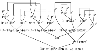
Figure 11: the IMLL proof net $\Theta_{4}$ obtained from $\Theta_{3}$ by applying the multiplicative $\eta$-expansion three time

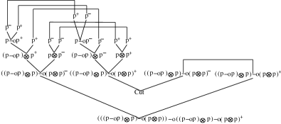
Figure 12: another example of IMLL proof nets with Cut-links $\Theta^{\prime}_{1}$

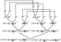
Figure 13: the IMLL proof net $\Theta^{\prime}_{2}$ obtained from $\Theta^{\prime}_{1}$ by the ID rewrite rule

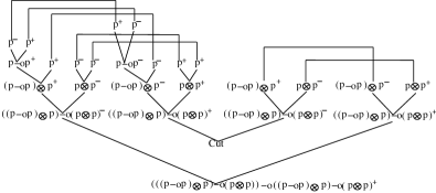
Figure 14: the IMLL proof net $\Theta^{\prime}_{3}$ obtained from $\Theta^{\prime}_{1}$ by the multiplicative $\eta$-expansion 1

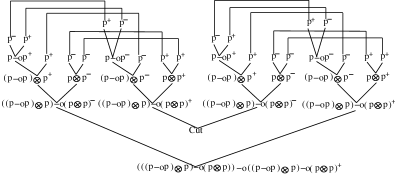
Figure 15: the IMLL proof net $\Theta^{\prime}_{4}$ obtained from $\Theta^{\prime}_{3}$ by applying the multiplicative $\eta$-expansion three time

Definition 5 (the maximal $\eta$-expansion of an ID-link)

Let $\Theta$ be the IMLL proof net consisting of exactly one ID-link with $A^{+}$ and $A^{-}$ as the conclusions. The maximal $\eta$-expansion of $\Theta$ is the IMLL proof net exactly with $A^{+}$ and $A^{-}$ as the conclusions that does not have any ID-links except ID-links with only atomic conclusions obtained from $\Theta$ by applying multiplicative $\eta$-expansion rules maximally. We denote the $\eta$-expansion of $\Theta$ by $\eta$-expand($A^{+},A^{-}$).

Lemma 1

Let $\Pi$ be an IMLL proof net with $A^{+}$ (respectively $A^{-}$) as a conclusion. Then we let $\Theta$ be the IMLL proof net connecting $\Pi$ and $\eta$-expand($A^{+},A^{-}$) by a Cut-link with $A^{+}$ (respectively $A^{-}$) on $\Pi$ and $A^{-}$ (respectively $A^{+}$) on $\eta$-expand($A^{+},A^{-}$) as the premises. Then there is an IMLL proof net $\Pi^{\prime}$ such that $\Pi\to^{\ast}\Pi^{\prime}$ and $\Theta\to^{\ast}\Pi^{\prime}$, where $\Pi^{\prime}$ is an IMLL proof net obtained from $\Pi$ by applying the multiplicative $\eta$-expansion to some (possibly zero) subformula occurrences of $A^{+}$ (resp. $A^{-}$) of $\Pi$.

Proof.    We prove this lemma by induction on $A^{+}$ (resp. $A^{-}$). We only consider $A^{+}$. The case of $A^{-}$ is similar.

1. The base step: the case where $A^{+}$ is an atomic formula $p^{+}$.
   Then $\eta$-expand($A^{+},A^{-}$) is an IMLL proof net consisting exactly one ID-link with $p^{+},p^{-}$ as the conclusions. Then we can easily see that $\Theta\to\Pi$ by ID rewrite rule. So, it is OK to let $\Pi^{\prime}$ be $\Pi$.

2. The induction step: the case where $A^{+}$ is not an atomic formula.

   1. the case where $A^{+}$ on $\Pi$ is a conclusion of an ID-link:
      Let $\Pi^{\prime}$ be the IMLL proof net obtained from $\Pi$ by replacing the ID-link with $\eta$-expand($A^{+},A^{-}$). Then $\Pi\to^{\ast}\Pi^{\prime}$. Moreover it is easily see to $\Theta\to\Pi^{\prime}$ by the ID rewrite rule.

   2. the case where $A^{+}$ on $\Pi$ is not a conclusion of an ID-link:

      1. the case where $A^{+}$ is a conclusion of $\bindnasrepma$-link:
         Then $A^{+}$ must have the form ${A_{1}\mathop{-\circ}A_{2}}^{+}$. Let $\Theta^{\prime}$ be the IMLL proof net such that $\Theta\to\Theta^{\prime}$ by the multiplicative rewrite rule 1. Then the graph $\Theta^{\prime\prime}$ obtained from $\Theta^{\prime}$ by removing $\bindnasrepma$-link with the conclusion ${A_{1}\mathop{-\circ}A_{2}}^{+}$ is a subproof net of $\Theta^{\prime}$. Then $\Theta^{\prime\prime}$ can be regarded as an IMLL proof net obtained from an IMLL proof net and $\eta$-expand($A_{1}^{+},A_{1}^{-}$) by connecting a Cut-link. Let $\Pi_{1}$ be the IMLL proof net obtained from $\Theta^{\prime\prime}$ by removing $\eta$-expand($A_{1}^{+},A_{1}^{-}$) and its associated Cut-link. By inductive hypothesis, we can obtain an IMLL proof net $\Pi^{\prime}_{1}$ such that $\Pi_{1}\to^{\ast}\Pi^{\prime}_{1}$ and $\Theta^{\prime}\to^{\ast}\Pi^{\prime}_{1}$, where $\Pi^{\prime}_{1}$ is obtained from $\Pi_{1}$ by applying the multiplicative $\eta$-expansion to some subformula occurrences of $A_{1}^{-}$ of $\Pi_{1}$. Again $\Pi^{\prime}_{1}$ can be regarded as an IMLL proof net obtained from an IMLL proof net and $\eta$-expand($A_{2}^{+},A_{2}^{-}$) by connecting a Cut-link. Let $\Pi_{2}$ be the IMLL proof net obtained from $\Pi^{\prime}_{1}$ by removing $\eta$-expand($A_{2}^{+},A_{2}^{-}$) and its associated Cut-link. By inductive hypothesis again, we can obtain an IMLL proof net $\Pi^{\prime}_{2}$ such that $\Pi_{2}\to^{\ast}\Pi^{\prime}_{2}$ and $\Pi^{\prime}_{1}\to^{\ast}\Pi^{\prime}_{2}$, where $\Pi^{\prime}_{2}$ is obtained from $\Pi_{2}$ by applying the multiplicative $\eta$-expansion to some subformula occurrences of $A_{2}^{+}$ of $\Pi_{1}$. Finally let the IMLL proof net obtained from $\Pi^{\prime}_{2}$ by adding $\bindnasrepma$-link with the conclusion ${A_{1}\mathop{-\circ}A_{2}}^{+}$ be $\Pi^{\prime}$. It can be easily seen that $\Theta\to^{\ast}\Pi^{\prime}$, $\Pi\to^{\ast}\Pi^{\prime}$, and $\Pi^{\prime}$ is obtained from $\Pi$ by applying the multiplicative $\eta$-expansion to some subformula occurrences of ${A_{1}\mathop{-\circ}A_{2}}^{+}$ of $\Pi$.

      2. the case where $A^{+}$ is a conclusion of $\otimes$-link:
         Then $A^{+}$ must have the form ${A_{1}\otimes A_{2}}^{+}$. Let $\Theta^{\prime}$ be the IMLL proof net such that $\Theta\to\Theta^{\prime}$ by the multiplicative rewrite rule 2. On the other hand there is an IMLL subproof net $\Pi_{1}$ (resp. $\Pi_{2}$) of $\Pi$ (and also of $\Theta^{\prime}$) such that $\Pi_{1}$ (resp. $\Pi_{2}$) is the maximal subproof net of $\Pi$ among the subproof nets with with a conclusion $A_{1}^{+}$ (resp. $A_{2}^{+}$). Let the IMLL proof net obtained by connecting $\Pi_{1}$ (resp. $\Pi_{2}$) and $\eta$-expand($A_{1}^{+},A_{1}^{-}$) (resp. $\eta$-expand($A_{2}^{+},A_{2}^{-}$)) by a Cut-link be $\Theta_{1}$ (resp. $\Theta_{2}$). $\Theta_{1}$ and $\Theta_{2}$ is also an IMLL subproof net of $\Theta^{\prime}$. By applying inductive hypothesis to $\Theta_{1}$ (resp. $\Theta_{2}$) and $\Pi_{1}$ (resp. $\Pi_{2}$), we obtain $\Pi^{\prime}_{1}$ (resp. $\Pi^{\prime}_{2}$) from $\Pi_{1}$ (resp. $\Pi_{2}$) by some $\eta$-expansions such that $\Pi_{1}\to^{\ast}\Pi^{\prime}_{1}$ (resp. $\Pi_{2}\to^{\ast}\Pi^{\prime}_{2}$) and $\Theta_{1}\to^{\ast}\Pi^{\prime}_{1}$ (resp. $\Theta_{2}\to^{\ast}\Pi^{\prime}_{2}$). The IMLL proof net obtained from $\Theta^{\prime}$ by replacing $\Theta_{1}$ and $\Theta_{2}$ by $\Pi^{\prime}_{1}$ and $\Pi^{\prime}_{2}$ is an IMLL proof net obtained from $\Pi$ by applying the multiplicative $\eta$-expansion to some subformula occurrences of ${A_{1}\otimes A_{2}}^{+}$ of $\Pi$.

$\Box$

Lemma 2 (Weak Confluence)

In the IMLL system we assume that $\Theta\to\Theta_{1}$ and $\Theta\to\Theta_{2}$. Then there is an IMLL proof net $\Theta_{3}$ such that $\Theta_{1}\to^{\ast}\Theta_{3}$ and $\Theta_{2}\to^{\ast}\Theta_{3}$.

Proof.    The problematic cases are four critical pairs in Figure 16. Let $\Theta_{1}$ be the left contractum in the pairs and $\Theta_{2}$ be the right contractum. Then we let $\Theta^{\prime}_{1}$ be the IMLL proof net obtained from $\Theta_{1}$ by applying the multiplicative $\eta$-expansion to $\Theta_{1}$ until there are no any ID-links with non-atomic conclusions. Note that $\Theta_{1}\to^{\ast}\Theta_{1}$. Next we apply Lemma 1 to $\Theta^{\prime}_{1}$. Then we can find $\Theta_{3}$ such that $\Theta_{2}\to^{\ast}\Theta_{3}$. Hence $\Theta^{\prime}_{1}\to^{\ast}\Theta_{3}$. $\Box$

Proposition 2 (Confluence)

The IMLL system is confluent.

Proof.    From Proposition 1 and Lemma 2 by Newman’s Lemma. $\Box$

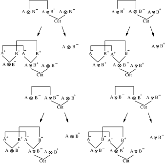
Figure 16: all the critical pairs

3 An equality on closed IMLL proof nets

In this section, we define an equality on closed IMLL proof nets.

Definition 6

An IMLL proof net $\Theta$ is closed if $\Theta$ has exactly one conclusion.

Next we consider the forms of normal IMLL proof nets. Let $\Theta$ be a normal IMLL proof net with the positive conclusion $A^{+}$ and the other conclusions $B_{1}^{-},\cdots,B_{n}^{-}$.

We consider the unique abstract syntax forest $T(A^{+}),T(B_{1}^{-}),\cdots,T(B_{n}^{-})$ determined by $A^{+},B_{1}^{-},\cdots,B_{n}^{-}$, where $T(A^{+})$ (resp. $T(B_{i}^{-})$ $\,(1\leq i\leq n)$) is the unique abstract syntax tree determined by $A^{+}$ (resp. $B_{i}^{-}$ $\,(1\leq i\leq n)$). For example, when let $A^{+}$ be ${p\mathop{-\circ}(p\otimes p)\mathop{-\circ}((p\mathop{-\circ}p\otimes p)\otimes(p\otimes p))}^{+}$, Figure 17 is the abstract syntax tree $T(A^{+})$.
Then we define a set ${\bf P}_{\Theta}$ of alternating sequences of nodes of the forest $T(A^{+}),T(B_{1}^{-}),\cdots,T(B_{n}^{-})$ and $\{{\bf L},{\bf R},{\bf ID}\}$ as follows:

1. $A^{+}\in{\bf P}_{\Theta}$;

2. If $s,{A_{1}\otimes A_{2}}^{+}\in{\bf P}_{\Theta}$, where $s$ is an alternating sequence, then $s,{A_{1}\otimes A_{2}}^{+},{\bf L},A_{1}^{+}\in{\bf P}_{\Theta}$ and $s,{A_{1}\otimes A_{2}}^{+},{\bf R},A_{2}^{+}\in{\bf P}_{\Theta}$;

3. If $s,{A_{1}\mathop{-\circ}A_{2}}^{+}\in{\bf P}_{\Theta}$, then $s,{A_{1}\mathop{-\circ}A_{2}}^{+},{\bf R},A_{2}^{+}\in{\bf P}_{\Theta}$;

4. If $s,p^{+}\in{\bf P}_{\Theta}$, then $s,p^{+},{\bf ID},p^{-}\in{\bf P}_{\Theta}$;

5. If $s,{A^{\prime}}^{-}\in{\bf P}_{\Theta}$ and ${A^{\prime}}^{-}$ is the right premise of a $\otimes^{-}$-link $L$, then $s,{A^{\prime}}^{-},{\bf R},{{A^{\prime\prime}}\otimes{A^{\prime}}}^{-}\in{\bf P}_{\Theta}$, where ${{A^{\prime\prime}}\otimes{A^{\prime}}}^{-}$ is the conclusion of $L$;

6. If $s,{A^{\prime}}^{-}\in{\bf P}_{\Theta}$ and ${A^{\prime}}^{-}$ is the left premise of a $\bindnasrepma^{-}$-link $L$, then $s,{A^{\prime}}^{-},{\bf L},{{A^{\prime}}\bindnasrepma{A^{\prime\prime}}}^{-}\in{\bf P}_{\Theta}$, where ${{A^{\prime}}\bindnasrepma{A^{\prime\prime}}}^{-}$ is the conclusion of $L$;

7. If $s,{A^{\prime}}^{-}\in{\bf P}_{\Theta}$ and ${A^{\prime}}^{-}$ is the right premise of a $\bindnasrepma^{-}$-link $L$, then $s,{A^{\prime}}^{-},{\bf R},{{A^{\prime\prime}}\bindnasrepma{A^{\prime}}}^{-}\in{\bf P}_{\Theta}$, where ${{A^{\prime\prime}}\bindnasrepma{A^{\prime}}}^{-}$ is the conclusion of $L$.

We say that $s,B^{-}\in{\bf P}_{\Theta}$ is a main path of $\Theta$, if $B^{-}$ is neither a premise of $\otimes^{-}$-link nor $\bindnasrepma^{-}$-link in $\Theta$. Then we call $B^{-}$ the head of the main path. Note that if $\Theta$ is an IIMLL proof net, then $\Theta$ has exactly one main path. If the positive conclusion of a subproof net of $\Theta$ is the left premise of a $\otimes^{-}$-link in a main path, then we call the subproof net a direct subproof net of $\Theta$.
For example, Figure 18 shows a closed IMLL proof net of ${p\mathop{-\circ}(p\otimes p)\mathop{-\circ}((p\mathop{-\circ}p\otimes p)\otimes(p\otimes p))}^{+}$, where we give abbreviations to some formula occurrences. There are exactly four main paths in the IMLL proof net:

1. $A^{+},{\bf R},A_{1}^{+},{\bf R},A_{2}^{+},{\bf L},A_{3}^{+},{\bf R},{p\otimes p}^{+},{\bf L},p^{+},{\bf ID},p^{-}$

2. $A^{+},{\bf R},A_{1}^{+},{\bf R},A_{2}^{+},{\bf L},A_{3}^{+},{\bf R},{p\otimes p}^{+},{\bf R},p^{+},{\bf ID},p^{-},{\bf R},{p\otimes p}^{-}$

3. $A^{+},{\bf R},A_{1}^{+},{\bf R},A_{2}^{+},{\bf R},{p\otimes p}^{+},{\bf L},p^{+},{\bf ID},p^{-},{\bf L},{p\otimes p}^{-}$

4. $A^{+},{\bf R},A_{1}^{+},{\bf R},A_{2}^{+},{\bf R},{p\otimes p}^{+},{\bf R},p^{+},{\bf ID},p^{-}$

The head of the path (3) is ${p\otimes p}^{-}$. Note that there is no direct subproof net of the IMLL proof net.

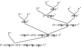
Figure 17: the abstract syntax tree of ${p\mathop{-\circ}(p\otimes p)\mathop{-\circ}((p\mathop{-\circ}p\otimes p)\otimes(p\otimes p))}^{+}$

Figure 18: a closed IMLL proof net of ${p\mathop{-\circ}(p\otimes p)\mathop{-\circ}((p\mathop{-\circ}p\otimes p)\otimes(p\otimes p))}^{+}$

Next, we define an equality on normal IMLL proof nets. Since we define IMLL proof nets inductively, it seems a reasonable definition that two proof nets are equal, if these are the same w.r.t forms and orders of applied rules in Figure 2. But if we defined an equality in this way, then there would be two different IMLL proof nets with the form of Figure 19, since there are two orders of applied rules in order to define the IMLL proof net. Because this is unreasonable, we define an equality in the following way.

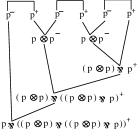
Figure 19: an IMLL proof net

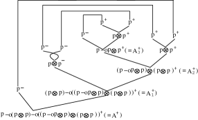
Figure 20: another closed IMLL proof net of ${p\mathop{-\circ}(p\otimes p)\mathop{-\circ}((p\mathop{-\circ}p\otimes p)\otimes(p\otimes p))}^{+}$

Definition 7 (an equality on normal IMLL proof nets)

Let $\Theta_{1}$ and $\Theta_{2}$ be two normal IMLL proof nets with the same positive conclusion. Then $\Theta_{1}=\Theta_{2}$ if

1. For each main path of $\Theta_{1}$ there is completely the same main path in $\Theta_{2}$. Moreover there is no any path in $\Theta_{2}$ other than these corresponding paths, i.e., there is a bijection from the set of the main paths of $\Theta_{1}$ to that of $\Theta_{2}$, which can be regarded as an identity map and

2. The head of a main path in $\Theta_{1}$ is a premise of a $\bindnasrepma^{+}$-link $L^{\prime}$ iff the corresponding head of $\Theta_{2}$ is also a premise of the $\bindnasrepma^{+}$-link $L^{\prime\prime}$ with the same position as $L^{\prime}$ and

3. If a direct subproof net of $\Theta_{1}$ is $\Theta^{\prime}$ and the corresponding subproof net of $\Theta_{2}$ is $\Theta^{\prime\prime}$, then $\Theta^{\prime}=\Theta^{\prime\prime}$ and

4. A head of a subproof net of $\Theta_{1}$ is a premise of a $\bindnasrepma^{+}$-link $L^{\prime}$ in a main path of $\Theta_{1}$ iff that of the corresponding subproof net of $\Theta_{2}$ is also a premise of the $\bindnasrepma^{+}$-link $L^{\prime\prime}$ with the same position as $L^{\prime}$.

For example, the IIMLL proof net of Figure 18 (let the net be $\Theta_{1}$) and that of Figure 20 (let the net be $\Theta_{2}$) are two IMLL proof nets with the same conclusion. But $\Theta_{1}\neq\Theta_{2}$, because there is no corresponding path in $\Theta_{2}$ to the path $A^{+},{\bf R},A_{1}^{+},{\bf R},A_{2}^{+},{\bf R},{p\otimes p}^{+},{\bf L},p^{+},{\bf ID},p^{-},{\bf L},{p\otimes p}^{-}$ in $\Theta_{1}$.
If the structure of proof nets is forgotten and collapses to the usual lambda calculus (see [Gir98]), our equality corresponds to the union of the usual $\beta\eta$-equality and the equivalence up to bijective replacement of free variables. But also note that our equality is not that of proof nets as graphs: for example, if we consider graphs whose nodes are links and whose edges are formulas (i.e., Danos-Regnier style’s proof-nets, see [DR95]), those of Figure 18 and Figure 20 are equal, because such graphs have no information about whether a premise of a link is left or right. On the other hand, it has a subtle point to extend our equality to the fragment including the multiplicative constant ${\bf 1}$: the topic will be given elsewhere.

4 Third-order reduction on IIMLL proof nets

In this section and the next section we only consider IIMLL proof nets. We assume that we are given two closed IIMLL proof nets $\Theta_{1}$ and $\Theta_{2}$ with the same conclusion such that $\Theta_{1}\neq\Theta_{2}$. In this section we show that we can find a context $C[]$ such that $C[\Theta_{1}]$ and $C[\Theta_{2}]$ have different normal forms and orders less than 4-th order.

Definition 8 (hole axioms)

A hole axiom with the positive conclusion $A^{+}$ is a link with the form shown by Figure 21.

Figure 21: one-hole axiom link

Definition 9 (extended IIMLL proof nets and one-hole contexts)

Extended IIMLL proof nets are inductively defined by using the rules of Figure 2 except for clauses (4) and (6) and that of Figure 22. A one-hole context (for short context) is an extended IIMLL proof net with exactly one one-hole axiom.

We use $C[],C_{0}[],C_{1}[],\ldots$ to denote one-hole contexts.

Remark.    Unlike [Bar84], there is no capture of free variables with regard to our notion of contexts, since we are working on closed proof nets.

Figure 22: extended IIMLL proof nets

Definition 10

Let $\Theta$ be an IIMLL proof net with the positive conclusion $A^{+}$ and $C[]$ be a one-hole context with the one-hole axiom $A^{+}$. Then $C[\Theta]$ is an IIMLL proof net obtained from $C[]$ by replacing one-hole axiom $A^{+}$ by $\Theta$.

Definition 11 (depth)

The depth of an IIMLL proof net $\Theta$ (denoted by $\mathop{\rm depth}\nolimits(\Theta)$) is inductively defined as follows:

1. If the main path of $\Theta$ does not include $\otimes^{-}$-links, then $\mathop{\rm depth}\nolimits(\Theta)$ is $1$.

2. Otherwise, when all the direct subproof nets of $\Theta$ are $\Theta_{1},\ldots,\Theta_{m}$, $\mathop{\rm depth}\nolimits(\Theta)$ is $\mathop{\rm max}\nolimits\{\mathop{\rm depth}\nolimits(\Theta_{1}),\ldots,\mathop{\rm depth}\nolimits(\Theta_{m})\}+1$.

The depth of a positive formula occurrence $A^{+}$ in $\Theta$ is $\mathop{\rm depth}\nolimits(\Theta)-\mathop{\rm depth}\nolimits(\Theta^{\prime})+1$, where $\Theta^{\prime}$ is the subproof net of $\Theta$ which is the least among subproof nets including $A^{+}$.

Definition 12 (the order of a positive IIMLL formula)

The order of an IIMLL formula $A^{+}$, denoted by $\mathop{\rm order}\nolimits(A^{+})$ is inductively as follows:

1. If $A^{+}$ is an atomic formula $p^{+}$ then $\mathop{\rm order}\nolimits(A^{+})$ is $1$.

2. If $A^{+}$ is ${A_{1}\mathop{-\circ}\ldots\mathop{-\circ}A_{n}\mathop{-\circ}p}^{+}$, then $\mathop{\rm order}\nolimits(A^{+})$ is

   $$\mathop{\rm max}\nolimits\{\mathop{\rm order}\nolimits(A_{1}^{+}),\ldots,\mathop{\rm order}\nolimits(A_{n}^{+})\}+1.$$

We define the order of a closed IIMLL proof net $\Theta$ as the order of the positive conclusion.

Definition 13 (the measure w.r.t linear implication)

Let $\Theta$ be an IIMLL proof net. The measure of $\Theta$ w.r.t linear implication denoted by $\mathop{\rm measure}\nolimits_{\mathop{-\circ}}(\Theta)$ is the sum of depths of all the positive formula occurrences of $\Theta$.

Lemma 3

Let $\Theta$ be an IIMLL proof net with the positive conclusion

$${A_{n}\mathop{-\circ}\ldots\mathop{-\circ}(B_{m}\mathop{-\circ}\ldots\mathop{-\circ}(C_{2}\mathop{-\circ}C_{1})\mathop{-\circ}\ldots\mathop{-\circ}B_{1}\mathop{-\circ}p)\mathop{-\circ}\ldots\mathop{-\circ}A_{1}\mathop{-\circ}p}^{+}$$

and the form shown in Figure 23. Then there is an IIMLL proof net with the positive conclusion

$${C_{2}\mathop{-\circ}A_{n}\mathop{-\circ}\ldots\mathop{-\circ}(B_{m}\mathop{-\circ}\ldots\mathop{-\circ}C_{1}\mathop{-\circ}\ldots\mathop{-\circ}B_{1}\mathop{-\circ}p)\mathop{-\circ}\ldots\mathop{-\circ}A_{1}\mathop{-\circ}p}^{+}.$$

Proof.    The proof structure of Figure 24 obtained from Figure 23 by manipulating some links is also an IIMLL proof net (the invisible part of $\Theta$ is never touched), because all the Danos-Regnier graphs of the IMLL proof structure of Figure 24 can be regarded as a subset of that of Figure 23 in the following way:

• In the $\bindnasrepma$-link with the conclusion ${C_{2}\mathop{-\circ}A_{n}\mathop{-\circ}\ldots\mathop{-\circ}(B_{m}\mathop{-\circ}\ldots\mathop{-\circ}C_{1}\mathop{-\circ}\ldots\mathop{-\circ}B_{1}\mathop{-\circ}p)\mathop{-\circ}\ldots\mathop{-\circ}A_{1}\mathop{-\circ}p}^{+}$, if $C_{2}^{-}$ is chosen, then identify $C_{2}^{-}$ with the conclusion of the $\bindnasrepma$-link;

• otherwise, identify the other premise with the conclusion of the $\bindnasrepma$-link.

If the proof structure of Figure 24 were not an IMLL proof net, that is, did not satisfy the criterion of Theorem 1, then $\Theta$ would not be an IMLL proof net by Theorem 1. This is a contradiction. $\Box$

Figure 23: An IIMLL proof net before reduced

Figure 24: The IIMLL proof net after reduced

Proposition 3

Let $\Theta_{1}$ and $\Theta_{2}$ be two closed IIMLL proof nets with the same positive conclusion and an order greater than 3 such that $\Theta_{1}\neq\Theta_{2}$. Then there is a context $C[]$ such that $\mathop{\rm measure}\nolimits_{\mathop{-\circ}}(\Theta_{1})>\mathop{\rm measure}\nolimits_{\mathop{-\circ}}(C[\Theta_{1}])$, $\mathop{\rm measure}\nolimits_{\mathop{-\circ}}(\Theta_{2})>\mathop{\rm measure}\nolimits_{\mathop{-\circ}}(C[\Theta_{2}])$, and $C[\Theta_{1}]\neq C[\Theta_{2}]$.

Proof.    Since $\Theta_{1}$ has an order greater than 3, the positive conclusion of $\Theta_{1}$ has the form

$${A_{n}\mathop{-\circ}\ldots\mathop{-\circ}(B_{m}\mathop{-\circ}\ldots\mathop{-\circ}B_{k+1}\mathop{-\circ}(C_{2}\mathop{-\circ}C_{1})\mathop{-\circ}B_{k-1}\mathop{-\circ}\ldots\mathop{-\circ}B_{1}\mathop{-\circ}p)\mathop{-\circ}\ldots\mathop{-\circ}A_{1}\mathop{-\circ}p}^{+}$$

for some $k$ ($1\leq k\leq m$).

On the other hand, there is an IIMLL proof net that is $\eta$-expansion of ID-link with the conclusion

$${A_{n}\mathop{-\circ}\ldots\mathop{-\circ}(B_{m}\mathop{-\circ}\ldots\mathop{-\circ}B_{k+1}\mathop{-\circ}(C_{2}\mathop{-\circ}C_{1})\mathop{-\circ}B_{k-1}\mathop{-\circ}\ldots\mathop{-\circ}B_{1}\mathop{-\circ}p)\mathop{-\circ}\ldots\mathop{-\circ}A_{1}\mathop{-\circ}p}^{-}$$

and

$${A_{n}\mathop{-\circ}\ldots\mathop{-\circ}(B_{m}\mathop{-\circ}\ldots\mathop{-\circ}B_{k+1}\mathop{-\circ}(C_{2}\mathop{-\circ}C_{1})\mathop{-\circ}B_{k-1}\mathop{-\circ}\ldots\mathop{-\circ}B_{1}\mathop{-\circ}p)\mathop{-\circ}\ldots\mathop{-\circ}A_{1}\mathop{-\circ}p}^{+}.$$

Then by Lemma 3 we can obtain an IIMLL proof net $\Pi$ whose conclusions are exactly

$${A_{n}\mathop{-\circ}\ldots\mathop{-\circ}(B_{m}\mathop{-\circ}\ldots\mathop{-\circ}B_{k+1}\mathop{-\circ}(C_{2}\mathop{-\circ}C_{1})\mathop{-\circ}B_{k-1}\mathop{-\circ}\ldots\mathop{-\circ}B_{1}\mathop{-\circ}p)\mathop{-\circ}\ldots\mathop{-\circ}A_{1}\mathop{-\circ}p}^{-}$$

and

$${C_{2}\mathop{-\circ}A_{n}\mathop{-\circ}\ldots\mathop{-\circ}(B_{m}\mathop{-\circ}\ldots\mathop{-\circ}B_{k+1}\mathop{-\circ}C_{1}\mathop{-\circ}B_{k-1}\mathop{-\circ}\ldots\mathop{-\circ}B_{1}\mathop{-\circ}p)\mathop{-\circ}\ldots\mathop{-\circ}A_{1}\mathop{-\circ}p}^{+}.$$

Then let $C[]$ be the context obtained from $\Pi$ by connecting $\Pi$’s negative conclusion and one-hole axiom via Cut-link. Then the number of the positive formula occurrences of $\Theta_{1}$ is equal to that of $C[\Theta_{1}]$. The positive formula occurrence ${C_{1}\mathop{-\circ}C_{2}}^{+}$ occurs in $\Theta_{1}$ and depth $2$, but not in $C[\Theta_{1}]$, while the positive formula occurrence

$${C_{2}\mathop{-\circ}A_{n}\mathop{-\circ}\ldots\mathop{-\circ}(B_{m}\mathop{-\circ}\ldots\mathop{-\circ}B_{k+1}\mathop{-\circ}C_{1}\mathop{-\circ}B_{k-1}\mathop{-\circ}\ldots\mathop{-\circ}B_{1}\mathop{-\circ}p)\mathop{-\circ}\ldots\mathop{-\circ}A_{1}\mathop{-\circ}p}^{+}$$

occurs in $C[\Theta_{1}]$ and has depth $1$, but not in $\Theta_{1}$. The other formula occurrences in $\Theta_{1}$ are the same as that of $C[\Theta_{1}]$. So, it is obvious that $\mathop{\rm measure}\nolimits_{\mathop{-\circ}}(\Theta_{1})>\mathop{\rm measure}\nolimits_{\mathop{-\circ}}(C[\Theta_{1}]).$

Note that in Proposition 3 the construction of $C[]$ only depends on the selection of a positive subformula occurrence of $\Theta_{1}$. Since $\Theta_{2}$ has a closed IIMLL proof net with the same positive conclusion of $\Theta_{1}$, we can easily see that $\mathop{\rm measure}\nolimits_{\mathop{-\circ}}(\Theta_{2})>\mathop{\rm measure}\nolimits_{\mathop{-\circ}}(C[\Theta_{2}])$.

Next in order to prove $C[\Theta_{1}]\neq C[\Theta_{2}]$, we consider the following cases:

1. the case where the $\bindnasrepma^{+}$-link of $\Theta_{1}$ and that of $\Theta_{2}$ to be manipulated by $C[]$ does not contribute to the unequality of $\Theta_{1}$ and $\Theta_{2}$:
   It is obvious $C[\Theta_{1}]\neq C[\Theta_{2}]$ since $C[]$ does not influence the rest.

2. the case where the $\bindnasrepma^{+}$-link of $\Theta_{1}$ and that of $\Theta_{2}$ to be manipulated by $C[]$ contributes to the unequality of $\Theta_{1}$ and $\Theta_{2}$:
   Then, the negative premise of the $\bindnasrepma^{+}$-link in $\Theta_{1}$ differs from that in $\Theta_{2}$ (as occurrences). Since the position in $C[\Theta_{1}]$ of the manipulated $\bindnasrepma^{+}$-link by $C[]$ is the same as that in $C[\Theta_{2}]$ and the position in $C[\Theta_{1}]$ of the premise of the $\bindnasrepma^{+}$-link differs that in $C[\Theta_{2}]$, it is obvious $C[\Theta_{1}]\neq C[\Theta_{2}]$. $\Box$

Example 1

Let $\Theta_{1}$ be the IIMLL proof net shown in the left side of Figure 25. Then $\mathop{\rm measure}\nolimits_{\mathop{-\circ}}(\Theta_{1})=10$. From Proposition 3 we obtain the context shown in Figure 26. By applying the context to $\Theta_{1}$ and normalizing the resulting net, we obtain the IIMLL proof net $\Theta_{2}$ shown in the right side of Figure 25. Then $\mathop{\rm measure}\nolimits_{\mathop{-\circ}}(\Theta_{2})=9$.

Figure 25: An IIMLL proof net before reduced and the IIMLL proof net after reduced

Figure 26: A context

Corollary 1

Let $\Theta_{1}$ and $\Theta_{2}$ be closed IIMLL proof nets with the same positive conclusion and an order greater than 3 such that $\Theta_{1}\neq\Theta_{2}$. Then there is a context $C[]$ such that $C[\Theta_{1}]\neq C[\Theta_{2}]$ and both have an order less than 4.

Proof.    By Proposition 3 we find a natural number $n$ ($n>0$) and a sequence of contexts $C_{1}[],C_{2}[],\ldots,C_{n}[]$ such that $C_{1}[C_{2}[\ldots C_{n}[\Theta_{1}]\ldots]]\neq C_{1}[C_{2}[\ldots C_{n}[\Theta_{2}]\ldots]]$ and both have an order less than 4. Then it is obvious that there is a context $C[]$ such that $C[\Theta]=C_{1}[C_{2}[\ldots C_{n}[\Theta]\ldots]]$ for any IIMLL proof net $\Theta$ with the same positive conclusion as $\Theta_{1}$ and $\Theta_{2}$. $\Box$

5 Value separation in third-order IIMLL proof nets

We assume that we are given two different normal IIMLL proof nets $\Theta_{1}$ and $\Theta_{2}$ with the same conclusion and with an order less than 4. However, we can not perform a separation directly. We need type instantiation.

Definition 14 (Type instantiation)

Let $\Theta$ be an IIMLL proof net and $A$ be an MLL formula. The type instantiated proof net $\Theta[A/p]$ of $\Theta$ w.r.t $A$ is an IIMLL proof net obtained from $\Theta$ by replacing each atomic formula occurrence $p$ by $A$.

In the following, given two closed IIMLL proof nets $\Theta_{1}$ and $\Theta_{2}$ with the same conclusion and with an order less than 4 such that $\Theta_{1}\neq\Theta_{2}$, we consider two type instantiated proof nets $\Theta_{1}[{\scriptstyle p\mathop{-\circ}(p\mathop{-\circ}p)\mathop{-\circ}(p\mathop{-\circ}p)\mathop{-\circ}p}/p]$ and $\Theta_{2}[{\scriptstyle p\mathop{-\circ}(p\mathop{-\circ}p)\mathop{-\circ}(p\mathop{-\circ}p)\mathop{-\circ}p}/p]$.

5.1 The definable functions on $p\mathop{-\circ}(p\mathop{-\circ}p)\mathop{-\circ}(p\mathop{-\circ}p)\mathop{-\circ}p$

Figure 27 shows the two closed normal proof nets on $p\mathop{-\circ}(p\mathop{-\circ}p)\mathop{-\circ}(p\mathop{-\circ}p)\mathop{-\circ}p$. We call the left proof net $\underline{0}$ and the right one $\underline{1}$. We discuss the definable functions on $\{\underline{0},\underline{1}\}$ in proof nets.

Figure 27: the two normal forms on $p\mathop{-\circ}(p\mathop{-\circ}p)\mathop{-\circ}(p\mathop{-\circ}p)\mathop{-\circ}p$

There are 20 closed normal proof nets of ${\scriptstyle(p\mathop{-\circ}(p\mathop{-\circ}p)\mathop{-\circ}(p\mathop{-\circ}p)\mathop{-\circ}p)\mathop{-\circ}(p\mathop{-\circ}(p\mathop{-\circ}p)\mathop{-\circ}(p\mathop{-\circ}p)\mathop{-\circ}p)}$. Then we can easily see that all the one-argument functions on $\{\underline{0},\underline{1}\}$ are definable by these proof nets. Table 1 shows these definable functions. As to two-argument functions, there are 112 closed normal proof nets of
${\scriptstyle(p\mathop{-\circ}(p\mathop{-\circ}p)\mathop{-\circ}(p\mathop{-\circ}p)\mathop{-\circ}p)\mathop{-\circ}(p\mathop{-\circ}(p\mathop{-\circ}p)\mathop{-\circ}(p\mathop{-\circ}p)\mathop{-\circ}p)\mathop{-\circ}(p\mathop{-\circ}(p\mathop{-\circ}p)\mathop{-\circ}(p\mathop{-\circ}p)\mathop{-\circ}p)}$. For example, Figure 28 shows such a proof net. The 112 proof nets define six two-argument functions on $\{\underline{0},\underline{1}\}$. Table 2 shows these six functions. In general, for any $n\,(n\geq 1)$, all the closed normal proof nets on

$${\scriptstyle\overbrace{\scriptstyle(p\mathop{-\circ}(p\mathop{-\circ}p)\mathop{-\circ}(p\mathop{-\circ}p)\mathop{-\circ}p)\mathop{-\circ}\ldots\mathop{-\circ}(p\mathop{-\circ}(p\mathop{-\circ}p)\mathop{-\circ}(p\mathop{-\circ}p)\mathop{-\circ}p)}^{n}\mathop{-\circ}(p\mathop{-\circ}(p\mathop{-\circ}p)\mathop{-\circ}(p\mathop{-\circ}p)\mathop{-\circ}p)}$$

define $2n+2$ functions. We can define

1. two constant functions that always return $\underline{0}$ or $\underline{1}$,

2. $n$ projection functions, which return the value of an argument directly, and

3. $n$ functions that are the negation of a projection function.

On the other hand, the number of all the $n$-argument functions on $\{\underline{0},\underline{1}\}$ is $2^{2^{n}}$. Although we only have very limited number of definable functions, nevertheless we can establish a separation result.

Remark.    In the following discussions, we identify an IIMLL formula with an another IIMLL formula that is different only up to a permutation: for example, $p\mathop{-\circ}(p\mathop{-\circ}p)\mathop{-\circ}(p\mathop{-\circ}p)\mathop{-\circ}p$ and $(p\mathop{-\circ}p)\mathop{-\circ}p\mathop{-\circ}(p\mathop{-\circ}p)\mathop{-\circ}p$. If we restrict IIMLL formulas to IIMLL formulas with an order less than 4 and only with occurrences of only one atomic formula $p$, we find that there are only two IIMLL formulas that have exactly two closed normal IIMLL proof nets, that is, $p\mathop{-\circ}(p\mathop{-\circ}p)\mathop{-\circ}(p\mathop{-\circ}p)\mathop{-\circ}p$ and $p\mathop{-\circ}p\mathop{-\circ}(p\mathop{-\circ}p\mathop{-\circ}p)\mathop{-\circ}p$. But unlike $p\mathop{-\circ}(p\mathop{-\circ}p)\mathop{-\circ}(p\mathop{-\circ}p)\mathop{-\circ}p$, we can not obtain our separation result by instantiating $p\mathop{-\circ}p\mathop{-\circ}(p\mathop{-\circ}p\mathop{-\circ}p)\mathop{-\circ}p$ for a propositional variable: Only two functions are definable by closed IIMLL proof nets of ${\scriptstyle(p\mathop{-\circ}p\mathop{-\circ}(p\mathop{-\circ}p\mathop{-\circ}p)\mathop{-\circ}p)\mathop{-\circ}(p\mathop{-\circ}p\mathop{-\circ}(p\mathop{-\circ}p\mathop{-\circ}p)\mathop{-\circ}p)}$, that is, $e_{3}$ and $e_{4}$ of Table 1. We can not define the two constant functions $e_{1}$ and $e_{2}$. Without these constant functions, we can not separate two closed proof nets of Figure 27 by instantiating $p\mathop{-\circ}p\mathop{-\circ}(p\mathop{-\circ}p\mathop{-\circ}p)\mathop{-\circ}p$ for $p$. That is, for any context $C[]$ with ${p\mathop{-\circ}p\mathop{-\circ}(p\mathop{-\circ}p\mathop{-\circ}p)\mathop{-\circ}p}^{+}$ as the conclusion, $C[\underline{0}[{\scriptstyle p\mathop{-\circ}p\mathop{-\circ}(p\mathop{-\circ}p\mathop{-\circ}p)\mathop{-\circ}p}/p]]=C[\underline{1}[{\scriptstyle p\mathop{-\circ}p\mathop{-\circ}(p\mathop{-\circ}p\mathop{-\circ}p)\mathop{-\circ}p}/p]]$. This is a justification of our choice of $p\mathop{-\circ}(p\mathop{-\circ}p)\mathop{-\circ}(p\mathop{-\circ}p)\mathop{-\circ}p$.

Figure 28: a normal form on $\scriptstyle{(p\mathop{-\circ}(p\mathop{-\circ}p)\mathop{-\circ}(p\mathop{-\circ}p)\mathop{-\circ}p)\mathop{-\circ}(p\mathop{-\circ}(p\mathop{-\circ}p)\mathop{-\circ}(p\mathop{-\circ}p)\mathop{-\circ}p)\mathop{-\circ}(p\mathop{-\circ}(p\mathop{-\circ}p)\mathop{-\circ}(p\mathop{-\circ}p)\mathop{-\circ}p)}$

$e_{1}(\underline{0})=\underline{0}$	$e_{2}(\underline{0})=\underline{1}$	$e_{3}(\underline{0})=\underline{0}$	$e_{4}(\underline{0})=\underline{1}$
$e_{1}(\underline{1})=\underline{0}$	$e_{2}(\underline{1})=\underline{1}$	$e_{3}(\underline{1})=\underline{1}$	$e_{4}(\underline{1})=\underline{0}$

Table 1: all the definable functions on ${\scriptstyle(p\mathop{-\circ}(p\mathop{-\circ}p)\mathop{-\circ}(p\mathop{-\circ}p)\mathop{-\circ}p)\mathop{-\circ}(p\mathop{-\circ}(p\mathop{-\circ}p)\mathop{-\circ}(p\mathop{-\circ}p)\mathop{-\circ}p)}$

$f_{1}(\underline{0},\underline{0})=\underline{0}$	$f_{2}(\underline{0},\underline{0})=\underline{1}$	$f_{3}(\underline{0},\underline{0})=\underline{0}$
$f_{1}(\underline{1},\underline{0})=\underline{0}$	$f_{2}(\underline{1},\underline{0})=\underline{1}$	$f_{3}(\underline{1},\underline{0})=\underline{0}$
$f_{1}(\underline{0},\underline{1})=\underline{0}$	$f_{2}(\underline{0},\underline{1})=\underline{1}$	$f_{3}(\underline{0},\underline{1})=\underline{1}$
$f_{1}(\underline{1},\underline{1})=\underline{0}$	$f_{2}(\underline{1},\underline{1})=\underline{1}$	$f_{3}(\underline{1},\underline{1})=\underline{1}$
$f_{4}(\underline{0},\underline{0})=\underline{1}$	$f_{5}(\underline{0},\underline{0})=\underline{0}$	$f_{6}(\underline{0},\underline{0})=\underline{1}$
$f_{4}(\underline{1},\underline{0})=\underline{1}$	$f_{5}(\underline{1},\underline{0})=\underline{1}$	$f_{6}(\underline{1},\underline{0})=\underline{0}$
$f_{4}(\underline{0},\underline{1})=\underline{0}$	$f_{5}(\underline{0},\underline{1})=\underline{0}$	$f_{6}(\underline{0},\underline{1})=\underline{1}$
$f_{4}(\underline{1},\underline{1})=\underline{0}$	$f_{5}(\underline{1},\underline{1})=\underline{1}$	$f_{6}(\underline{1},\underline{1})=\underline{0}$

Table 2: all the definable functions by 112 closed normal proof nets on ${\scriptstyle(p\mathop{-\circ}(p\mathop{-\circ}p)\mathop{-\circ}(p\mathop{-\circ}p)\mathop{-\circ}p)\mathop{-\circ}(p\mathop{-\circ}(p\mathop{-\circ}p)\mathop{-\circ}(p\mathop{-\circ}p)\mathop{-\circ}p)\mathop{-\circ}(p\mathop{-\circ}(p\mathop{-\circ}p)\mathop{-\circ}(p\mathop{-\circ}p)\mathop{-\circ}p)}$

5.2 Separation

The main purpose of the subsection is to prove the following theorem.

Theorem 2

Let $\Theta_{1}$ and $\Theta_{2}$ be IIMLL proof nets with the same conclusion and with an order less than 4 such that $\Theta_{1}\neq\Theta_{2}$. Then there is a context $C[]$ such that
$C[\Theta_{1}[{\scriptstyle p\mathop{-\circ}(p\mathop{-\circ}p)\mathop{-\circ}(p\mathop{-\circ}p)\mathop{-\circ}p}/p]]=\underline{0}$ and $C[\Theta_{2}[{\scriptstyle p\mathop{-\circ}(p\mathop{-\circ}p)\mathop{-\circ}(p\mathop{-\circ}p)\mathop{-\circ}p}/p]]=\underline{1}$.

In order to prove the theorem, we need some preparations.
At first we remark that given a closed normal IIMLL proof net $\Theta$ with an order less than 4, we can associate a composition $F$ of second order variables $G_{1},\ldots G_{m}$, where each $G_{i}$ ($1\leq i\leq m$) occurs in $F$ linearly and corresponds to a second order negative formula occurrence in the conclusion of $\Theta$ and, the way that $G_{1},\ldots,G_{m}$ compose is determined by the structure of $\Theta$ (we can easily define $F$ inductively on the depth of $\Theta$).
Let $A^{-}$ be a second order negative IIMLL formula, that is, $A$ has the form $\overbrace{p\mathop{-\circ}\cdots\mathop{-\circ}p}^{n}\mathop{-\circ}p$. Then we define $\mathop{\rm arity}\nolimits(A)$ as $n$.

Proposition 4

Let $\Theta$ be a normal closed IIMLL proof net with an order less than 4, $A_{1}^{-},\ldots,A_{m}^{-}$ be the second order negative formula occurrences in the conclusion of $\Theta$, and $n$ be the number of all the occurrences of $p^{-}$ in the conclusion of $\Theta$. Moreover, let $g_{1},\ldots,g_{m}$ be functions such that each $g_{i}\,(1\leq i\leq m)$ is definable by a closed proof net on

$$\scriptstyle{\overbrace{\scriptstyle(p\mathop{-\circ}(p\mathop{-\circ}p)\mathop{-\circ}(p\mathop{-\circ}p)\mathop{-\circ}p)\mathop{-\circ}\ldots\mathop{-\circ}(p\mathop{-\circ}(p\mathop{-\circ}p)\mathop{-\circ}(p\mathop{-\circ}p)\mathop{-\circ}p)}^{\mathop{\rm arity}\nolimits(A_{i})}\mathop{-\circ}(p\mathop{-\circ}(p\mathop{-\circ}p)\mathop{-\circ}(p\mathop{-\circ}p)\mathop{-\circ}p)},$$

$c_{1},\ldots,c_{n}$ be a sequence of $\{\underline{0},\underline{1}\}$, and $f$ be the linear composition of $g_{1},\ldots,g_{m}$ corresponding to $\Theta$. Then there is a context $C[]$ such that $C[\Theta[{\scriptstyle p\mathop{-\circ}(p\mathop{-\circ}p)\mathop{-\circ}(p\mathop{-\circ}p)\mathop{-\circ}p}/p]]\to^{\ast}c$ iff $f(c_{1},\ldots,c_{n})=c$, where $c$ is an element of $\{\underline{0},\underline{1}\}$.

Proof.    The conclusion of $\Theta[{\scriptstyle p\mathop{-\circ}(p\mathop{-\circ}p)\mathop{-\circ}(p\mathop{-\circ}p)\mathop{-\circ}p}/p]$ has the form

$B_{k}\mathop{-\circ}\cdots\mathop{-\circ}B_{1}\mathop{-\circ}(p\mathop{-\circ}(p\mathop{-\circ}p)\mathop{-\circ}(p\mathop{-\circ}p)\mathop{-\circ}p)$. Moreover, each $B_{i}\,(1\leq i\leq k)$ has a closed IIMLL proof net $\Theta_{i}$ with the conclusion $B_{i}^{+}$ corresponding to any of $g_{1},\ldots,g_{m}$ or $c_{1},\ldots c_{n}$. Then we can construct an context $C[]$ shown in Figure 29. $\Box$

Figure 29: a context

We note that the construction of $C[]$ only depends on the conclusion on $\Theta$, not on $\Theta$ itself.

Proof of Theorem 2.   We know by Proposition 4 that we can identify a context $C[]$ with an assignment of definable functions on $\{\underline{0},\underline{1}\}$ and values in $\{\underline{0},\underline{1}\}$ to the two linear compositions $F_{1}$ and $F_{2}$ corresponding to $\Theta_{1}$ and $\Theta_{2}$. Since the conclusion of $\Theta_{1}$ is the same as that of $\Theta_{2}$, $F_{1}$ and $F_{2}$ are different expressions such that

1. each variable $x_{j}\,(1\leq j\leq n)$ occurs linearly in both $F_{1}$ and $F_{2}$ and

2. each second order variable $G_{i}\,(1\leq i\leq m)$ also occurs linearly in both $F_{1}$ and $F_{2}$.

We consider the two cases depending on the way $\Theta_{1}$ and $\Theta_{2}$ differ:

1. the case where there are $i\,(1\leq i\leq m)$ and $j_{1}$ and $j_{2}\,(1\leq j_{1},j_{2}\leq n)$ such that $G_{i}(\ldots,x_{j_{1}},\ldots)$ occurs in $F_{1}$ and $G_{i}(\ldots,x_{j_{2}},\ldots)$ occurs in $F_{2}$ and $j_{1}\neq j_{2}$, where $x_{j_{1}}$ and $x_{j_{2}}$ have the same position in $G_{i}$:
   Then, there is $G_{i^{\prime}}$ with the least depth among such $G_{i}$’s. Note that the expression $F_{1}$ (resp. $F_{2}$) can be regarded as a tree and the path from $G_{i^{\prime}}$ to the root of $F_{1}$ is the same as that of $F_{2}$. To each $G_{k}$ occurrence in the path we assign the projection function w.r.t the argument selected by the path. To other $G_{k^{\prime}}$ we assign the constant function that always returns $\underline{0}$. In addition, we assign $\underline{0}$ (resp. $\underline{1}$) to $x_{j_{1}}$ (resp. $x_{j_{2}}$). To other $x_{k}$ we assign $\underline{0}$. Then it is obvious that by the assignment $F_{1}$ (resp. $F_{2}$) returns $\underline{0}$ (resp. $\underline{1}$).

2. otherwise:
   There is $i\,(1\leq i\leq m)$ such that the position of $G_{i}$ in $F_{1}$ differs from that of $F_{2}$. Then, there is $G_{i^{\prime}}$ with the least depth among such $G_{i}$’s in $F_{1}$ or $F_{2}$. Without loss of generality, we can assume that $G_{i^{\prime}}$ in $F_{1}$ has the least depth. Then to $G_{i^{\prime}}$ we assign the constant function that always returns $\underline{1}$. Again note that the expression $F_{1}$ (resp. $F_{2}$) can be regarded as a tree and the path from immediately outer $G_{\ell}$ of $G_{i^{\prime}}$ to the root of $F_{1}$ is the same as that of $F_{2}$. To each $G_{k}$ occurrence in the path we assign the projection function w.r.t the argument selected by the path. To other $G_{k^{\prime}}$ we assign the constant function that always returns $\underline{0}$. To any $x_{k}$ we assign $\underline{0}$. Then it is obvious that by the assignment $F_{1}$ (resp. $F_{2}$) returns $\underline{1}$ (resp. $\underline{0}$). $\Box$

Corollary 2 (Weak Typed Böhm Theorem on IIMLL)

Let $\Theta_{1}$ and $\Theta_{2}$ be IIMLL proof nets with the same conclusion such that $\Theta_{1}\neq\Theta_{2}$. Then there is a context $C[]$ such that $C[\Theta_{1}[{\scriptstyle p\mathop{-\circ}(p\mathop{-\circ}p)\mathop{-\circ}(p\mathop{-\circ}p)\mathop{-\circ}p}/p]]=\underline{0}$ and $C[\Theta_{2}[{\scriptstyle p\mathop{-\circ}(p\mathop{-\circ}p)\mathop{-\circ}(p\mathop{-\circ}p)\mathop{-\circ}p}/p]]=\underline{1}$.

Proof.    By Corollary 1 and Theorem 2. $\Box$

In the following we explain the proof of Theorem 2 by two examples.

Example 2

We explain the case (1) of the proof of Theorem 2, using Figure 30. Let $\Theta_{1}$ (resp. $\Theta_{2}$) be the left (resp. right) IIMLL proof net of Figure 30. The expression $F_{1}$ (resp. $F_{2}$) corresponding to $\Theta_{1}$ (resp. $\Theta_{2}$) is $G_{1}(G_{2}(x_{5},G_{4}(x_{4},x_{3})),G_{3}(x_{2},x_{1}))$ (resp. $G_{1}(G_{2}(x_{5},G_{4}(x_{1},x_{3})),G_{3}(x_{2},x_{4}))$). Then we pay attention to the second argument of $G_{3}$, that is, $x_{1}$ of $F_{1}$ and $x_{4}$ of $F_{2}$, because the argument in $F_{1}$ is not the same as that of $F_{2}$ and $G_{3}$ has the least depth among such second order variables. Following the proof, we let the context $C[]$ be the corresponding to the assignment [$x_{1}=\underline{0}$, $x_{2}=\underline{0}$, $x_{3}=\underline{0}$, $x_{3}=\underline{0}$, $x_{4}=\underline{1}$, $x_{5}=\underline{0}$, $G_{1}=f_{3}$, $G_{2}=f_{1}$, $G_{3}=f_{3}$, $G_{4}=f_{1}$] (see Table 2). Then $C[\Theta_{1}]\to^{\ast}\underline{0}$ and $C[\Theta_{2}]\to^{\ast}\underline{1}$.

Example 3

We explain the case (2) of the proof of Theorem 2, using Figure 31 and Figure 32. Let $\Theta_{1}$ (resp. $\Theta_{2}$) be the IIMLL proof net of Figure 31 (resp. Figure 32). The expression $F_{1}$ (resp. $F_{2}$) corresponding to $\Theta_{1}$ (resp. $\Theta_{2}$) is
$G_{1}(H_{3}(x_{4}),G_{2}(H_{2}(H_{1}(x_{3})),G_{3}(x_{2},x_{1})))$ (resp. $G_{1}(H_{3}(x_{4}),G_{2}(H_{2}(G_{3}(x_{2},x_{1})),H_{1}(x_{3})))$). Then we pay attention to the $G_{3}$ and $H_{1}$ that have the position in the second argument of $G_{2}$ in $F_{1}$ and $F_{2}$ respectively, because the second argument of $G_{2}$ in $F_{1}$ are not the same as that of $F_{2}$ and $G_{2}$ has the least depth among such second order variables. Following the proof, we let the context $C[]$ be the corresponding to the assignment [$x_{1}=\underline{0}$, $x_{2}=\underline{0}$, $x_{3}=\underline{0}$, $x_{4}=\underline{0}$, $G_{1}=f_{3}$, $G_{2}=f_{3}$, $G_{3}=f_{1}$, $H_{1}=e_{2}$, $H_{2}=e_{1}$, $H_{3}=e_{1}$ ] (see Table 1 and Table 2). Then $C[\Theta_{1}]\to^{\ast}\underline{0}$ and $C[\Theta_{2}]\to^{\ast}\underline{1}$.

Figure 30: an example of the case (1) of the proof of Theorem 2

Figure 31: an example of the case (2) of the proof of Theorem 2

Figure 32: an example of the case (2) of the proof of Theorem 2

6 An extension to the IMLL case

At first we define a special form of third-order IMLL formulas.

Definition 15 (simple third-order IMLL formulas)

An IMLL formula $A$ is simple if $A$ has the form $\displaystyle B_{1}\mathop{-\circ}\cdots\mathop{-\circ}B_{e}\mathop{-\circ}\overbrace{p\otimes\cdots\otimes p}^{d}\,\,(c\geq 0,d\geq 1,e\geq 0)$, where
$\displaystyle B_{i}=\overbrace{p\otimes\cdots\otimes p}^{k_{1}}\mathop{-\circ}\cdots\mathop{-\circ}\overbrace{p\otimes\cdots\otimes p}^{k_{\ell_{i}}}\mathop{-\circ}\overbrace{p\otimes\cdots\otimes p}^{m_{i}}\,\,(k_{j}\geq 0,1\leq j\leq\ell_{i},\ell_{i}\geq 1,m_{i}\geq 1,1\leq i\leq e)$.

Proposition 5

Let $\Theta_{1}$ and $\Theta_{2}$ be closed IMLL proof nets with the same positive conclusion such that $\Theta_{1}\neq\Theta_{2}$. Then there is a context $C[]$ such that $C[\Theta_{1}]\neq C[\Theta_{2}]$ and the positive conclusion of closed IMLL proof nets $C[\Theta_{1}]$ and $C[\Theta_{2}]$ is simple.

Proof.    Basically the same method as that of Corollary 1. $\Box$

For example, the same conclusion of two IMLL proof nets of Figure 18 and Figure 20 is not simple. By giving an appropriate context, we can transform these IMLL proof nets to two IMLL proof nets with a simple formula as the conclusion in Figure 33.

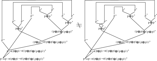
Figure 33: two different IMLL proof nets

Proposition 6

Let $\Theta_{1}$ and $\Theta_{2}$ be closed IMLL proof nets with the same positive simple conclusion such that $\Theta_{1}\neq\Theta_{2}$. Then there is a context $C[]$ such that $C[\Theta_{1}]\neq C[\Theta_{2}]$ and the positive conclusion of closed IIMLL proof nets $C[\Theta_{1}]$ and $C[\Theta_{2}]$ has an order less than 4.

Proof.    Let the positive simple conclusion of $\Theta_{1}$ and $\Theta_{2}$ be $A^{+}$ in Definition 15. Then it is obvious to be able to construct an IMLL proof net which has conclusions $A^{-}$ and $\displaystyle\overbrace{p\mathop{-\circ}\cdots\mathop{-\circ}p}^{\sum^{e}_{i=1}(m_{i}-1)}\mathop{-\circ}C_{1}\mathop{-\circ}\cdots\mathop{-\circ}C_{e}\mathop{-\circ}(\overbrace{p\mathop{-\circ}\cdots\mathop{-\circ}p}^{d}\mathop{-\circ}p)\mathop{-\circ}{p}^{+}$, where $\displaystyle C_{i}=\overbrace{p\mathop{-\circ}\cdots\mathop{-\circ}p}^{\sum_{j=1}^{\ell_{i}}k_{j}}\mathop{-\circ}p\,\,(1\leq i\leq e)$. It is also obvious to be able to construct a context $C[]$ such that $C[\Theta_{1}]\neq C[\Theta_{2}]$ and the positive conclusion of $C[\Theta_{1}]$ and $C[\Theta_{2}]$ is an intended IIMLL formula. $\Box$

For example, there is an IMLL proof net exactly with ${p_{4}\mathop{-\circ}p_{1}\mathop{-\circ}(p_{2}\otimes p_{3})\mathop{-\circ}((p_{5}\otimes p_{6})\otimes(p_{7}\otimes p_{8}))}^{-}$ and ${p_{2}\mathop{-\circ}p_{4}\mathop{-\circ}p_{1}\mathop{-\circ}p_{3}\mathop{-\circ}(p_{5}\mathop{-\circ}p_{6}\mathop{-\circ}p_{7}\mathop{-\circ}p_{8}\mathop{-\circ}p_{0})\mathop{-\circ}p_{0}}^{+}$ as the conclusions, where the indices of the atomic formula $p$ represent the pairings of ID-links. From the IMLL proof net, we can construct a context that transforms two IMLL proof nets of Figure 33 to two IIMLL proof nets of Figure 34.

Figure 34: two different IIMLL proof nets

From Proposition 5, Proposition 6, and Theorem 2, we obtain the following corollary.

Corollary 3 (Weak Typed Böhm Theorem on IMLL)

Let $\Theta_{1}$ and $\Theta_{2}$ be IMLL proof nets with the same conclusion such that $\Theta_{1}\neq\Theta_{2}$. Then there is a context $C[]$ such that $C[\Theta_{1}[{\scriptstyle p\mathop{-\circ}(p\mathop{-\circ}p)\mathop{-\circ}(p\mathop{-\circ}p)\mathop{-\circ}p}/p]]=\underline{0}$ and $C[\Theta_{2}[{\scriptstyle p\mathop{-\circ}(p\mathop{-\circ}p)\mathop{-\circ}(p\mathop{-\circ}p)\mathop{-\circ}p}/p]]=\underline{1}$.

7 Concluding remarks

Our result is easily extendable to IMLL with the multiplicative unit 1 under a reasonable equality on the extended system, because the multiplicative unit can be considered as a degenerated IMLL formula. For example ${\bf 1}^{+}$ has just one closed proof net and the closed proof nets on ${{\bf 1}\mathop{-\circ}p\mathop{-\circ}(p\mathop{-\circ}p)\mathop{-\circ}(p\mathop{-\circ}p)\mathop{-\circ}p}^{+}$ have almost the same behaviour as that of ${p\mathop{-\circ}(p\mathop{-\circ}p)\mathop{-\circ}(p\mathop{-\circ}p)\mathop{-\circ}p}^{+}$. However, our separation result w.r.t IMLL with 1 is stated as follows:

Let $\Theta_{1}$ and $\Theta_{2}$ be closed IMLL with 1 proof nets with the same positive conclusion such that $\Theta_{1}\neq\Theta_{2}$. Then there is a context $C[]$ such that $C[\Theta_{1}]$ and $C[\Theta_{2}]$ are closed proof nets of ${{\bf 1}\mathop{-\circ}{\bf 1}}^{+}$ and $C[\Theta_{1}]\neq C[\Theta_{2}]$.

There are two closed normal proof nets of ${{\bf 1}\mathop{-\circ}{\bf 1}}^{+}$: one consists of exactly three links (an axiom link for ${\bf 1}^{+}$, a weakening link for ${\bf 1}^{-}$, and a $\bindnasrepma$-link). Let the proof net be $\underline{{\tt ff}}_{{{\bf 1}\mathop{-\circ}{\bf 1}}^{+}}$. The other consists of exactly two links (an ID-link with ${\bf 1}^{-}$ and ${\bf 1}^{+}$ and a $\bindnasrepma$-link). Let the proof net be $\underline{{\tt tt}}_{{{\bf 1}\mathop{-\circ}{\bf 1}}^{+}}$. The proof is similar to that of IMLL without 1.
However in a symmetric monoidal closed category (SMCC, for example, see [MO03]), $\underline{{\tt ff}}_{{{\bf 1}\mathop{-\circ}{\bf 1}}^{+}}$ and $\underline{{\tt tt}}_{{{\bf 1}\mathop{-\circ}{\bf 1}}^{+}}$ are interpreted into the same arrow $id_{I}$, where $I$ is the multiplicative unit of a SMCC. To avoid such an identification, it is possible to relax conditions of SMCC: one is to remove the axiom $l_{I}=r_{I}$. The other is that we do not assume $I$ is isomorphic to $I\otimes I$; just we assume $I$ is a retract of $I\otimes I$, that is, we remove two axioms $l_{A};{l_{A}}^{-1}=id_{I\otimes A}$ and $r_{A};{r_{A}}^{-1}=id_{A\otimes I}$. The relaxation is quite natural: for example, without these axioms we can derive important equations like $\alpha_{I,A,B};l_{A\otimes B}=l_{A}\otimes id_{B}$. In the relaxed SMCC, proof nets of IMLL with 1 can be an internal language.
On the other hand, our result cannot be extended to classical multiplicative Linear Logic (for short MLL) directly, because all MLL proof nets cannot be polarized by IMLL polarity. For example, the MLL proof net of Figure 35 cannot be transformed to an IMLL proof net by type instantiation.
As an another direction, fragments including additive connectives may be studied. Currently it is proved that our method can be applied to a restricted fragment of intuitionistic multiplicative additive linear logic. The restriction is as follows:

1. With-formulas must positively occur only as $A\binampersand A$;

2. Plus-formulas must negatively occur only as $A\oplus A$.

Moreover we can also prove the strong statement of typed Böhm theorem w.r.t the fragment. Our ongoing work is to eliminate the restriction.

Figure 35: A counterexample

Appendix A A classification

In this appendix we classify the closed normal IIMLL proof nets of
${\scriptstyle\overbrace{\scriptstyle(p\mathop{-\circ}(p\mathop{-\circ}p)\mathop{-\circ}(p\mathop{-\circ}p)\mathop{-\circ}p)\mathop{-\circ}\ldots\mathop{-\circ}(p\mathop{-\circ}(p\mathop{-\circ}p)\mathop{-\circ}(p\mathop{-\circ}p)\mathop{-\circ}p)}^{n}\mathop{-\circ}(p\mathop{-\circ}(p\mathop{-\circ}p)\mathop{-\circ}(p\mathop{-\circ}p)\mathop{-\circ}p)}$. First we introduce a linear $\lambda$-term assignment system to normal IIMLL proof nets, since it is easier to discuss the classification in terms of $\beta\eta$-long normal linear $\lambda$-terms than in terms of normal IIMLL proof nets. Figure 36 shows the term assignment system. It is easy to see that all the assigned terms are linear and $\beta\eta$-long normal, because to each ID-link with atomic conclusions a different variable is assigned and the first argument in an application term introduced in rule (2) is always a variable.

Figure 36: A linear $\lambda$-term-assignment system

Second we consider the closed normal linear $\lambda$-terms assigned to ${p\mathop{-\circ}(p\mathop{-\circ}p)\mathop{-\circ}(p\mathop{-\circ}p)\mathop{-\circ}p}$. While the linear $\lambda$-term $\lambda x.\lambda f.\lambda g.g(fx)$ corresponds to the IIMLL proof net $\underline{0}$, $\lambda x.\lambda f.\lambda g.f(gx)$ corresponds to $\underline{1}$.

A.1 The closed normal terms on ${\scriptstyle(p\mathop{-\circ}(p\mathop{-\circ}p)\mathop{-\circ}(p\mathop{-\circ}p)\mathop{-\circ}p)\mathop{-\circ}(p\mathop{-\circ}(p\mathop{-\circ}p)\mathop{-\circ}(p\mathop{-\circ}p)\mathop{-\circ}p)}$

Next we classify the closed $\beta\eta$-long normal terms of
${\scriptstyle(p\mathop{-\circ}(p\mathop{-\circ}p)\mathop{-\circ}(p\mathop{-\circ}p)\mathop{-\circ}p)\mathop{-\circ}(p\mathop{-\circ}(p\mathop{-\circ}p)\mathop{-\circ}(p\mathop{-\circ}p)\mathop{-\circ}p)}$ as a preliminary step. Since the closed $\beta\eta$-long normal terms on the formula have always the form $\lambda F.\lambda x.\lambda f.\lambda g.t$, we only write down the body $t$ instead of writing down the whole term in the following.
We classify them according to the surrounding contexts of $f$ and $g$.

1. The case where $\lambda y.f(gy)$ or $\lambda y.g(fy)$ occurs as a subterm:
   (1) $Fx(\lambda y_{1}.y_{1})(\lambda y_{2}.f(gy_{2}))$ and (2) $Fx(\lambda y_{1}.y_{1})(\lambda y_{2}.g(fy_{2}))$ and
   (3) $Fx(\lambda y_{1}.f(gy_{1}))(\lambda y_{2}.y_{2})$ and (4) $Fx(\lambda y_{1}.g(fy_{1}))(\lambda y_{2}.y_{2})$

2. The case where both $\lambda y.fy$ and $\lambda y.gy$ occur as a subterm:
   (5) $Fx(\lambda y_{1}.fy_{1})(\lambda y_{2}.gy_{2})$ and (6) $Fx(\lambda y_{1}.gy_{1})(\lambda y_{2}.fy_{2})$
   While the first term denotes the identity function on $\{\underline{0},\underline{1}\}$, the second term the negation. The terms of the other cases are a constant function on $\{\underline{0},\underline{1}\}$. Note that in order for a term to denote a non-constant function, in the term, $f$ and $g$ must occur in the second argument and the third argument of $F$ separately, because for $F$, $\lambda x.\lambda f.\lambda g.g(fx)$ or $\lambda x.\lambda f.\lambda g.f(gx)$ is substituted.

3. The case where $\lambda y.fy$ (respectively $\lambda y.gy$) occurs as a subterm, but $\lambda y.gy$ (respectively $\lambda y.fy$) does not:
   (7) $f(Fx(\lambda y_{1}.y_{1})(\lambda y_{2}.gy_{2}))$ and (8) $g(Fx(\lambda y_{1}.y_{1})(\lambda y_{2}.fy_{2}))$ and
   (9) $f(Fx(\lambda y_{1}.gy_{1})(\lambda y_{2}.y_{2}))$ and (10) $g(Fx(\lambda y_{1}.fy_{1})(\lambda y_{2}.y_{2}))$ and
   (11) $F(fx)(\lambda y_{1}.y_{1})(\lambda y_{2}.gy_{2})$ and (12) $F(gx)(\lambda y_{1}.y_{1})(\lambda y_{2}.fy_{2})$ and
   (13) $F(fx)(\lambda y_{1}.gy_{1})(\lambda y_{2}.y_{2})$ and (14) $F(gx)(\lambda y_{1}.fy_{1})(\lambda y_{2}.y_{2})$.

4. The case where neither $\lambda y.f(gy)$, $\lambda y.g(fy)$, $\lambda y.fy$, nor $\lambda y.gy$ occurs as a subterm:
   (15) $f(g(Fx(\lambda y_{1}.y_{1})(\lambda y_{2}.y_{2})))$ and (16) $g(f(Fx(\lambda y_{1}.y_{1})(\lambda y_{2}.y_{2})))$ and
   (17) $f(F(gx)(\lambda y_{1}.y_{1})(\lambda y_{2}.y_{2}))$ and (18) $g(F(fx)(\lambda y_{1}.y_{1})(\lambda y_{2}.y_{2}))$ and
   (19) $F(f(gx))(\lambda y_{1}.y_{1})(\lambda y_{2}.y_{2})$ and (20) $F(g(fx))(\lambda y_{1}.y_{1})(\lambda y_{2}.y_{2})$

A.2 The general case

Finally, we classify the closed normal terms of
${\scriptstyle\overbrace{\scriptstyle(p\mathop{-\circ}(p\mathop{-\circ}p)\mathop{-\circ}(p\mathop{-\circ}p)\mathop{-\circ}p)\mathop{-\circ}\ldots\mathop{-\circ}(p\mathop{-\circ}(p\mathop{-\circ}p)\mathop{-\circ}(p\mathop{-\circ}p)\mathop{-\circ}p)}^{n}\mathop{-\circ}(p\mathop{-\circ}(p\mathop{-\circ}p)\mathop{-\circ}(p\mathop{-\circ}p)\mathop{-\circ}p)}$. Since the closed $\beta\eta$-long normal terms on the formula has always the form $\lambda F_{1}.\cdots\lambda F_{n}.\lambda x.\lambda f.\lambda g.t$, we only write down the body $t$ instead of writing down the whole term in the following.
The classification proceeds in the same fashion as that of the previous subsection:

1. The case where $\lambda y.f(gy)$ or $\lambda y.g(fy)$ occurs as a subterm:
   In this case, $t$ has the form

   $$F_{1}(\cdots(F_{n-1}(F_{n}\,\,x\,\,t_{2n-1}t_{2n})t_{2n-3}t_{2n-2})\cdots)t_{1}t_{2}$$

   or a permutation on $\{F_{1},\ldots,F_{n}\}$ of the form, where $t_{i}\,(1\leq i\leq 2n)$ is $\lambda y.f(gy)$, $\lambda y.g(fy)$ or $\lambda y.y$, but any of $\lambda y.f(gy)$ and $\lambda y.g(fy)$ exclusively occurs once. The total number of such terms is $n!\times 2\times 2n$.

2. The case where both $\lambda y.fy$ and $\lambda y.gy$ occur as a subterm:
   In this case, $t$ has the form

   $$F_{1}(\cdots(F_{n-1}(F_{n}\,\,x\,\,t_{2n-1}t_{2n})t_{2n-3}t_{2n-2})\cdots)t_{1}t_{2}$$

   or a permutation on $\{F_{1},\ldots,F_{n}\}$ of the form, where $t_{i}\,(1\leq i\leq 2n)$ is $\lambda y.fy$, $\lambda y.gy$ or $\lambda y.y$, and both $\lambda y.fy$ and $\lambda y.gy$ occur exactly once. The total number of such terms is $n!\times 2\times{\scriptstyle{2n}}C_{2}=n!\times 2\times\sum^{2n-1}_{k=1}k=n!\times 2\times(2n^{2}-n)$. Among such terms the total number of the terms in which there is an $i\,(1\leq i\leq n)$ such that both the second argument and the third argument of $F_{i}$ are exactly $\lambda y.fy$ or $\lambda y.gy$ is $n!\times 2\times n$. Only such limited terms are a non-constant function, i.e., a projection or the negation of such a projection. Other terms of the case and the terms of the other cases are a constant function.

3. The case where $\lambda y.fy$ (respectively $\lambda y.gy$) occurs as a subterm, but $\lambda y.gy$ (respectively $\lambda y.fy$) does not:
   In this case, $t$ has the form

   $$h_{1}(F_{1}(h_{2}(F_{2}(\cdots(h_{n-1}(F_{n-1}(h_{n}(F_{n}(h_{n+1}x)t_{2n-1}t_{2n}))t_{2n-3}t_{2n-2}))\cdots)t_{3}t_{4}))t_{2}t_{1})$$

   or a permutation on $\{F_{1},\ldots,F_{n}\}$ of the form, where $h_{i}\,(1\leq i\leq n+1)$ is empty or $g$ (resp. $f$), and $g$ (resp. $f$) occurs exactly once. Moreover $t_{j}\,(1\leq j\leq 2n)$ is $\lambda y.y$ or $\lambda y.fy$ (resp. $\lambda y.gy$) and $\lambda y.fy$ (resp. $\lambda y.gy$) occurs exactly once. The total number of such terms is $n!\times 2\times((n+1)\times 2n)$.

4. The case where neither $\lambda y.f(gy)$, $\lambda y.g(fy)$, $\lambda y.fy$, nor $\lambda y.gy$ occurs as a subterm:
   In this case, $t$ has the form

   $$h_{1}(F_{1}(h_{2}(F_{2}(\cdots(h_{n-1}(F_{n-1}(h_{n}(F_{n}(h_{n+1}x)t_{2n-1}t_{2n}))t_{2n-3}t_{2n-2}))\cdots)t_{3}t_{4}))t_{2}t_{1})$$

   or a permutation on $\{F_{1},\ldots,F_{n}\}$ of the form, where $h_{i}\,(1\leq i\leq n+1)$ is empty, $f$, $g$, $f(g[])$, or $g(f[])$, and both $f$ and $g$ occur exactly once. Moreover $t_{j}\,(1\leq i\leq 2n)$ is always $\lambda y.y$. The total number of such terms is $n!\times 2\times\sum^{n+1}_{k=1}k=n!\times(n^{2}+3n+2)$.

References

- [Bar84] H. Barendregt. The Lambda Calculus: Its Syntax and Semantics, North Holland,1984.
- [DP00] Kosta Dosen and Zoran Petric. The Maximality of the Typed Lambda Calculus and of Cartesian Closed Categories. Publications de l’Institut Mathematique, 68(82), pp. 1-19, 2000.
- [DP01] Kosta Dosen and Zoran Petric. The Typed Bohm Theorem. Electronic Notes in Theoretical Computer Science, vol. 50, no. 2, Elsevier Science Publishers, 2001.
- [DR89] Vincent Danos and Laurent Regnier. The structure of multiplicatives. Archive for Mathematical Logic, 28:181-203, 1989.
- [DR95] Vincent Danos and Laurent Regnier. Proof-nets and Hilbert space. In J.-Y. Girard, Y. Lafont, and L. Regnier, editors, Advances in Linear Logic, pages 307-328. Cambridge University Press, 1995.
- [Gir87] J.-Y. Girard. Linear Logic. Theoretical Computer Science, 50:1-102, 1987.
- [Gir96] J.-Y. Girard. Proof-nets: the parallel syntax for proof-theory. In Ursini and Agliano, editors, Logic and Algebra, New York, Marcel Dekker, 1996.
- [Gir98] J.-Y. Girard. Light Linear Logic. Information and Computation, 143, 175–204, 1998.
- [Jol00] T. Joly. Codages, séparabilité et représentation de fonctions dans divers lambda-calculs typés. Thèse de doctorat, Université Paris VII, Jan. 2000.
- [LT04] O. Laurent and L. Tortora de Falco. Slicing polarized additive normalization. In T. Ehrhard,J.-Y. Girard,P. Ruet and P. Scott eds, Linear Logic in Computer Science, pp. 247-282, Cambridge University Press, 2004.
- [MO03] A.S. Murawski and C.-H.L. Ong. Exhausting strategies, joker games and full completeness for IMLL with Unit. Theoretical Computer Science, 294:269-305, 2003.
- [SP00] A. Simpson and G. Plotkin Complete axioms for categorical fixedpoint operators. LICS’2000, pp 30-41, 2000.
- [SD92] R. Statman and G. Dowek. On Statman’s Finite Completeness Theorem. Technical Report CMU-CS-92-152, Carnegie Mellon University, 1992.
- [Sta80] R. Statman. On the existence of closed terms in the typed lambda-calculus I. In Hindley, J. R. and Seldin, J. P. eds, To H. B. Curry Essays on Combinatory Logic, Lambda Calculus and Formalism, pp. 511-534, Academic Press, 1980.
- [Sta82] R. Statman. Completeness, Invariance and lambda-Definability. The Journal of Symbolic Logic, 47:17-26, 1982.
- [Sta83] R. Statman. -definable functionals and -conversion. Arch. math. Logik, 23:21-26. 1983.
- [TdF00] L. Tortora de Falco. Réseaux, cohérence et expériences obsessionnelles. Thèse de doctorat, Université Paris VII, Jan. 2000.
- [TdF03] L. Tortora de Falco. Obsessional experiments for Linear Logic Proof-nets. Mathematical Structures in Computer Science, 13:799-855,2003.