Life Above Threshold:
From List Decoding to Area Theorem and MSE

Life Above Threshold:
From List Decoding to Area Theorem and MSE

Cyril Méasson and Rüdiger Urbanke

EPFL, I&C
CH-1015 Lausanne, Switzerland
e-mail: cyril.measson@epfl.ch
ruediger.urbanke@epfl.ch

Andrea Montanari

LPTENS (UMR 8549, CNRS et ENS)
24, rue Lhomond, 75231
Paris CEDEX 05, France
e-mail: montanar@lpt.ens.fr

Tom Richardson

Flarion Technologies
Bedminster, NJ, USA-07921
e-mail: richardson@flarion.com

Abstract — We consider communication over memoryless channels using low-density parity-check code ensembles above the iterative (belief propagation) threshold. What is the computational complexity of decoding (i.e., of reconstructing all  the typical input codewords for a given channel output) in this regime? We define an algorithm accomplishing this task and analyze its typical performance. The behavior of the new algorithm can be expressed in purely information-theoretical terms. Its analysis provides an alternative proof of the area theorem for the binary erasure channel. Finally, we explain how the area theorem is generalized to arbitrary memoryless channels. We note that the recently discovered relation between mutual information and minimal square error is an instance of the area theorem in the setting of Gaussian channels.

I. Introduction

The analysis of iterative coding systems has been extremely effective in determining the conditions for successful communication. The single most important prediction in this context is the existence of a threshold noise level below which the bit error rate vanishes (as the blocklength and the number of iterations diverge). The threshold can be computed for a large variety of code ensembles using density evolution.

On the other hand, understanding the behavior of these systems above threshold is largely an open issue. Since in this regime the bit error rate remains bounded away from zero, one may wonder about the motivation for such an investigation. We can think of three possible answers: $(i)$ It is intellectually frustrating to have an “half-complete” theory of iterative decoding. Moreover this theory has poor connections with classical issues such as the behavior of the same codes under maximum likelihood (ML) decoding. $(ii)$ Loopy belief propagation has stimulated a considerable interest as a general-purpose inference algorithm for graphical models. However, there are very few applications where its effectiveness can be analyzed mathematically. Decoding below threshold is probably the most prominent of such examples and one may hope to build upon this success. $(iii)$ There are communication contexts in which one is is interested in reproducing some information within a pre-established tolerance, rather than exactly. There are indications that iterative methods can play an important role also in such contexts. If this is the case, one will necessarily operate in the above-threshold regime.

Consider, for the sake of simplicity, communication over a memoryless channel using random elements from a standard low-density parity-check (LDPC) code ensemble. Assume moreover that the noise level is greater than the threshold one. There are two natural theoretical problems one can address in this regime: (A) How many channel inputs correspond to a given typical output? (B) How hard is to reconstruct all of them? Answering question (A) amounts to computing the conditional entropy $H(X_{1}^{n}|Y_{1}^{n})$ of the channel input given the output (here $n$ is the blocklength). We expect this entropy to become of order $O(n)$ at large enough noise. We call the minimum noise level for this to be the case, the ML threshold. ML decoding is bound to fail above this threshold.

The second question is apparently far from Information Theory and in any case very difficult to answer. The naive expectation would be that reconstructing all the typical codewords becomes harder as their conditional entropy gets larger.

In this paper we report some recent progress on both of the questions outlined above. In Secs. Life Above Threshold: From List Decoding to Area Theorem and MSE and Life Above Threshold: From List Decoding to Area Theorem and MSE we reconsider the binary erasure channel (BEC). We define a natural extension of the belief propagation decoder which reconstruct all the codewords compatible with a given channel output. The new algorithm (‘Maxwell decoder’) thus performs a ‘complete’ list decoding, and is based on the general message-passing philosophy. Below the iterative threshold, it coincides with belief propagation decoding and its complexity is linear in the blocklength. Above the iterative threshold, its complexity becomes exponential. Its behavior can be analyzed precisely, and provides answers both questions (A) and (B) above (within this circumscribed context). Surprisingly, the resulting picture is most easily conveyed using a well-known information theoretic characterization of the code: the ${\sf EXIT}$ curve. As a byproduct, we obtain an alternative proof of the area theorem for the BEC.

The connection between the ${\sf EXIT}$ curve and Maxwell decoder is not a peculiarity of the binary erasure channel, and has instead a rather fundamental origin. The algorithm progressively reduces the uncertainty on the transmitted bits. This can be regarded as an effective change of the noise level of the communication channel. The ${\sf EXIT}$ curve describe the response of the bits (i.e., the change of the bit uncertainty) to a change in the noise level. The area theorem is obtained when integrating this response: the total bit uncertainty at maximal noise level (the code rate) is thus given by an integral of the ${\sf EXIT}$ curve.

In Sec. Life Above Threshold: From List Decoding to Area Theorem and MSE, we explain how to generalize these ideas to arbitrary memoryless channels. In particular, we define a generalized ${\sf EXIT}$ function ${\sf GEXIT}$, which has the same important properties of the usual one. We show that an area theorem holds for such a function, implying, among other things, an upper bound on the ML threshold. ${\sf GEXIT}$ reduces to ${\sf EXIT}$ for the BEC and to the minimal mean-square error (${\sf MMSE}$) for additive Gaussian channels.

II. Area Theorem for the Binary Erasure Channel

Consider a degree distribution pair $(\lambda,\rho)$ and ensembles ${\rm LDPC}(n,\lambda,\rho)$ of increasing length $n$. Figure 1 shows a typical asymptotic ${\sf EXIT}$ function. Its main characteristics (for a regular ensemble with left degree at least 3) are as follows: The function is zero below the ML threshold $\epsilon_{\rm{ML}}$. It jumps at $\epsilon_{\rm{ML}}$ to a non-zero value and continues then smoothly until it reaches one for $\epsilon=1$. The area under the ${\sf EXIT}$ curve equals the rate of the code, see [5]. Compare this to the equivalent function of the iterative (IT) decoder which is also shown in Fig. 1. It is easy to check that this curve is given in parametric form by

$$\left(\frac{x}{\lambda(1-\rho(1-x))},\Lambda(1-\rho(1-x))\right),$$ (1)

where $x$ signifies the erasure probability of left-to-right messages. Equation (1) can be derived from the fixed-point equation $\epsilon\lambda(1-\rho(1-x))-x=0$. We express $\epsilon$ as $\epsilon(x)=\frac{x}{\lambda(1-\rho(1-x))}$ and notice that the average probability that a bit is still erased (ignoring the observation of the bit itself) at the fixed point is equal to $\Lambda(1-\rho(1-x))$. Note that the iterative curve is the trace of this parametric equation for $x$ starting at $x=1$ until $x=x_{\rm{IT}}$. This is the critical point and $\epsilon(x_{\rm{IT}})=\epsilon_{\rm{IT}}$. Summarizing, the iterative ${\sf EXIT}$ curve is zero up to the iterative threshold $\epsilon_{\rm{IT}}$. It then jumps to a non-zero value and also continues smoothly until it reaches one at $\epsilon=1$. Multiple jumps are possible in some irregular ensembles, but we shall neglect this possibility here.

The following two curious relationships between these two curves were shown in [1]. First, the IT and the ML curve coincide above $\epsilon_{\rm{ML}}$. Second, the ML curve can be constructed from the iterative curve in the following way. If we draw the IT curve as parametrized in Eq. (1) not only for $x\geq x_{\rm{IT}}$ but also for $0\leq x\leq x_{\rm{IT}}$ we get the curve shown in the right picture of Fig. 1. Notice that the branch $0\leq x\leq x_{\rm{IT}}$ describes an unstable fixed point under iterative decoding. Moreover the fraction of erased messages $x$ decreases along this branch when the erasure probability is increased. Finally it satisfies $x>\epsilon$. Because of these peculiar features, it is usually considered as “spurious”.

To determine the ML threshold take a straight vertical line at $\epsilon=\epsilon_{\rm{IT}}$ and shift it to the right until the area which lies to the left of this straight line and is enclosed by the line and the iterative curve is equal to the area which lies to the right of the line and is enclosed by the line and the iterative curve (these areas are indicated in dark gray in the picture). This unique point determines the ML threshold. The ML ${\sf EXIT}$ curve is now the curve which is zero to the left of the threshold and equals the iterative curve to the right of this threshold. In other words, the ML threshold is determined by a balance between two areas.

Figure 1: Left: The ${\sf EXIT}$ curve of the ML decoder for the degree distribution pair $(\lambda(x)=x^{2},\rho(x)=x^{5})$. The curve is zero until $\epsilon^{\rm{ML}}$ at which point it jumps. It then continuous smoothly until it reaches one at $\epsilon=1$. Also shown is the equivalent curve under iterative decoding. Right: The full iterative ${\sf EXIT}$ curve including the “spurious branch”. This corresponds to an unstable fixed point $x>\epsilon$. The ML threshold is determined by the balance of the two dark gray areas.

III. Maxwell Decoder

The balance condition described above, cf. Fig. 1, is strongly reminiscent of the so-called ‘Maxwell construction’ in statistical mechanics [8]. This allows, for instance, to determine the location of a liquid-gas phase transition, by balancing two areas in the pressure-volume phase diagram. The Maxwell construction is derived by considering a reversible transformation between the liquid and vapor phases. The balance condition follows from the observation that the net work exchange along such a transformation must vanish at the phase transition point.

Inspired by the statistical mechanics analogy, we shall explain the balance condition determining the ML threshold by analyzing an algorithm which moves from the non zero-entropy branch to the zero-entropy branch of the ${\sf EXIT}$ curve. To this end we construct a fictitious decoder, which for obvious reasons we name the Maxwell decoder. Instead of explaining the balance between the areas as shown in Fig. 1 we will explain the balance of the two areas shown in Fig. 2. Note that these two areas differ from the previous ones only by a common term so that the condition for balance stays unchanged.

Figure 2: ${\sf EXIT}$ curve for the $(x^{2},x^{5})$ ensemble. Dark gray: the two areas whose balance is proved by the analysis of the Maxwell decoder. Left: Total number of guesses made by a decoder starting at $\epsilon_{\rm ML}$ (divided by the blocklength). Right: Total number of contradictions encountered (divided by the blocklength).

Let us now introduce the decoder: Given the received word which was transmitted over the BEC$(\epsilon)$, the decoder proceeds iteratively as does the standard message passing decoder. At any time the iterative decoding process gets stuck in a non-empty stopping set the decoder randomly chooses a position $i\in[n]$. If this position is not known yet the decoder splits any running copy of the decoding process into two, one which proceed with the decoding process by assuming that $x_{i}={\tt 0}$ and one which proceeds by assuming that $x_{i}={\tt 1}$. This splitting procedure is repeated any time the decoder gets stuck and we say that the decoder guesses a bit. During the decoding it can happen that contradictions occur, i.e., that a variable node receives inconsistent messages. Any copy of the decoding process which contains such contradictions terminates. From the above description it follows that at any given point of the decoding process there are $2^{h(\ell)}$ copies alive, where $h(\ell)$ is a natural number which evolves with time $\ell$. Eventually, each surviving copies will has determined all the erased bits, and outputs the corresponding word of size $n$. It is hopefully clear from the above description that the final list of surviving copies is in one-to-one correspondence with the list of codewords that are compatible with the received message. In other words, the Maxwell decoder performs a complete list decoding of received message.

In Fig. 3 we depict an instance of the decoding process is shown from the perspective of the various simultaneous copies. The initial phase coincides with standard message passing: a single copy of the process decodes a bit at a time. After three steps, belief propagation gets stuck in stopping set and several steps of guessing follow. During this phase $h(\ell)$ (the associated entropy, i.e., the $\log_{2}$ of the number of simultaneously running copies) increases. After this guessing phase, the standard message passing phase resumes. More and more copies will terminate due to inconsistent messages (incorrect guesses). At the end, only one copy survives, which shows that the example has a unique ML solution.

Figure 3: Maxwell decoder applied to a simple example when the all-zero codeword is decoded.

In Fig. 4 we plot the entropy $h(\ell)$ as a function of the number of iterations for several code and channel realizations (here we consider a $(3,6)$ ensemble with blocklength $n=10^{4}$ and erasure probability $\epsilon=0.47$). It can be shown that the rescaled entropy $h(\ell)/n$ concentrates around a finite limiting value if we take the large blocklength limit $n\to\infty$, with $\ell/n$ fixed. Moreover the limiting curve can be computed exactly. Here we limit ourselves to outline the connection with the various areas highlighted in Fig. 2 and to explain why these areas should be in balance at the ML threshold. To simplify matters consider only channel parameters $\epsilon$ with $\epsilon\geq\epsilon_{\rm{IT}}$. We claim that the total number of guesses one has to venture during the guessing phase of the algorithm is equal to the dark gray area shown in the left picture of Fig. 2, i.e., it is equal to the integral under the iterative curve from $\epsilon_{\rm IT}$ up to $\epsilon$.

The effect of the guesses is to bring the effective erasure probability down from $\epsilon$ to $\epsilon_{\rm{IT}}$. At this point the standard message passing decoder can resume. The guesses are now resolved in the following manner. Assume that at some point in time there is a variable node which has $d$ connected check nodes of degree one. The corresponding incoming messages have to be consistent. This gives rise to $d-1$ constraints, or in other words, only a fraction $2^{d-1}$ of the running copies survive. It can now be shown that the total number of such constraints which are imposed is equal to the area in the left picture of Fig. 2. At the ML threshold all guesses have to be resolved at the end of the decoding process. This implies that the total number of required guesses has to equal the total number of resolved guesses which implies an equality of the areas as promised!

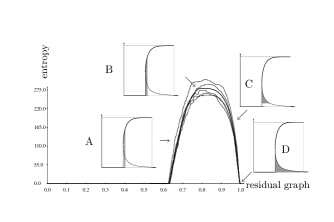
Figure 4: Entropy of the Maxwell decoder (logarithm of the number of running copies) as a function of the number of determined bits. We plot the results for several channel and code realizations (here for a $(3,6)$ ensemble with blocklength $n=10^{4}$ and $\epsilon=0.47$) together with the analytical asymptotic curve. In the inset: how the asymptotic curve can be constructed form the ${\sf EXIT}$ function.

Notice that the Maxwell decoder plays the same role as a reversible transformation in thermodynamics.

IV. General Channel

Three important lessons can be learned from the BEC example treated in the previous Sections. First of all: the ${\sf EXIT}$ curve gives the change in conditional entropy of the transmitted message when the channel noise level is incremented by an infinitesimal amount. Second: in a search algorithm reconstructing all the typical input codewords, this change has to be compensated for by an increase of the algorithm entropy. This is the fundamental reason of the equality between the area under the stable branch of the ${\sf EXIT}$ curve and the number of guesses made by the Maxwell decoder. Third: the fact that the iterative ${\sf EXIT}$ curve extends below the maximum-likelihood one implies that the corresponding additional guesses must be eventually resolved. The unstable branch of the ${\sf EXIT}$ curves yield the number of contradictions found in this resolution stage.

The first step towards a generalization of this scenario for an arbitrary memoryless channel consist in finding the appropriate generalization of the ${\sf EXIT}$ curve. We obtain such a generalization by enforcing the first of the above properties. For the sake of definiteness, we assume both the input and output alphabets to be finite and denote by $Q(y|x)$, $x\in{\cal X}$, $y\in{\cal Y}$ the transition probability. Formulae for continuous alphabets are easily obtained by substituting integrals $\int\!dx$, $\int\!dy$, to sums $\sum_{x}$, $\sum_{y}$. We moreover denote by $w$ a generic noise-level parameter and assume $Q(y|x)$ to be differentiable with respect to $w$. In analytical calculations, it is convenient to distinguish the noise levels for each channel use $w_{i}$, $i\in[n]$. The time-invariant channel is recovered by setting $w_{1}=\dots=w_{n}=w$ Finally, we denote by $\underline{X}\equiv X_{1}^{n}$ the channel input and $\underline{Y}\equiv Y_{1}^{n}$ the channel output. Our definition of a generalized ${\sf EXIT}$ curve is

$${\sf GEXIT}\equiv\frac{1}{n}\frac{d\phantom{w}}{dw}H(\underline{X}|\underline{Y})\,.$$ (2)

Notice that ${\sf GEXIT}$ satisfies the area theorem by construction: our purpose is to get a manageable expression for it. It is convenient to think of the above differentiation as acting on each channel separately

$${\sf GEXIT}=\frac{1}{n}\sum_{i=1}^{n}\frac{d\phantom{w}}{dw_{i}}H(\underline{X}|\underline{Y})\equiv\frac{1}{n}\sum_{i=1}^{n}{\sf GEXIT}_{i}\,,$$ (3)

with ${\sf GEXIT}_{i}$ defined as the derivative with respect to $w_{i}$. In order to compute ${\sf GEXIT}_{i}$, it is convenient to isolate the contribution of $X_{i}$ to the conditional entropy. If we denote by $Z_{i}$ the extrinsic information at $i$, and use the shorthands $\underline{X}^{[i]}\equiv(X_{j}\,:\,j\in[n]\backslash i)$, $\underline{Y}^{[i]}\equiv(Y_{j}\,:\,j\in[n]\backslash i)$, we get

$$H(\underline{X}|\underline{Y})=H(X_{i}|Z_{i},Y_{i})+H(\underline{X}^{[i]}|X_{i},\underline{Y}^{[i]})\,.$$ (4)

This is obtained by a standard application of the entropy chain rule

$$H(\underline{X}|\underline{Y}) = H(X_{i}|\underline{Y})+H(\underline{X}^{[i]}|X_{i},\underline{Y})$$

$$= H(X_{i}|\underline{Y},Z_{i})+H(\underline{X}^{[i]}|X_{i},\underline{Y}^{[i]})$$

$$= H(X_{i}|Y_{i},\underline{Y}^{[i]},Z_{i})+H(\underline{X}^{[i]}|X_{i},\underline{Y}^{[i]})$$

$$= H(X_{i}|Y_{i},Z_{i})+H(\underline{X}^{[i]}|X_{i},\underline{Y}^{[i]})\,.$$

We remark at this point that only the first term of the decomposition (4) depends upon the channel at position $i$. Therefore

$${\sf GEXIT}_{i}=\frac{d\phantom{w}}{dw_{i}}H(X_{i}|Z_{i},Y_{i})\,.$$ (5)

It is convenient to obtain a more explicit expression for the above formula. To this end we write

$$H(X_{i}|Z_{i},Y_{i}) = -\sum_{x_{i},y_{i},z_{i}}P(z_{i})P(x_{i}|z_{i})Q(y_{i}|x_{i})\cdot$$

$$\phantom{\sum_{x_{i},y_{i},z_{i}}}\cdot\log\left\{\frac{P(x_{i}|z_{i})Q(y_{i}|x_{i})}{\sum_{x_{i}^{\prime}\in{\cal X}}P(x^{\prime}_{i}|z_{i})Q(y_{i}|x^{\prime}_{i})}\right\}\,.$$

The dependence of $H(X_{i}|Z_{i},Y_{i})$ upon the channel at position $i$ is completely explicit and we can differentiate. The terms obtained by differentiating with respect to the channel inside the log vanish. For instance, when differentiating with respect to the $Q(y_{i}|x_{i})$ at the numerator, we get

$$-\sum_{x_{i},y_{i},z_{i}}P(z_{i})P(x_{i}|z_{i})\frac{d\phantom{w}}{dw_{i}}Q(y_{i}|x_{i})$$

$$= -\sum_{x_{i},z_{i}}P(z_{i})P(x_{i}|z_{i})\frac{d\phantom{w}}{dw_{i}}\sum_{y_{i}}Q(y_{i}|x_{i})=0\,.$$

We thus proved the following

Theorem 1

With the above definitions

$${\sf GEXIT}_{i} = \sum_{x_{i},y_{i},z_{i}}P(x_{i})P(z_{i}|x_{i})Q^{\prime}(y_{i}|x_{i})\cdot$$

$$\phantom{\sum_{x_{i},y_{i},z_{i}}}\cdot\log\left\{\sum_{x^{\prime}_{i}}\frac{P(x^{\prime}_{i}|z_{i})Q(y_{i}|x^{\prime}_{i})}{P(x_{i}|z_{i})Q(y_{i}|x_{i})}\right\}\,,$$

where we denoted by $Q^{\prime}(y|x)$ the derivative of the channel transition probability with respect to the noise level $w$.

The interest of the above result is that it encapsulates all our ignorance about the code behavior into the distribution of extrinsic information $P(z_{i})$. This is in turn the natural object appearing in message passing algorithms and in density evolution analysis. In order to fully appreciate the meaning of Eq. (1), it is convenient to consider a couple of more specific examples.

Linear Codes over BMS Channels

We assume the code to be linear and to be used over a binary-input memoryless output-symmetric (BMS) channel. We furthermore denote the channel input by ${\cal X}=\{{\tt 0},{\tt 1}\}$. This is the most common setting in the analysis of iterative coding systems. Exploiting the channel symmetry we can fix $x_{i}={\tt 0}$ in Eq. (1) and get

$${\sf GEXIT}_{i}=\sum_{y_{i},z_{i}}P_{0}(z_{i})Q^{\prime}(y_{i}|x_{i})\log\left\{1+\frac{P({\tt 1}|z_{i})Q(y_{i}|{\tt 1})}{P({\tt 0}|z_{i})Q(y_{i}|{\tt 0})}\right\}\,,$$

where we defined $P_{0}(z_{i})$ to be the distribution of the extrinsic information at $i$ under the condition that the all-zero codeword has been transmitted. Recall that $Z_{i}$ is a function of $\underline{Y}^{[i]}$ and $P_{0}(z_{i})$ is the distribution induced on $Z_{i}$ by the distribution of $\underline{Y}^{[i]}$.

It is convenient to encode the extrinsic information $z_{i}$ as an extrinsic log-likelihood ratio $l_{i}\equiv\log[P({\tt 0}|z_{i})/P({\tt 1}|z_{i})]$. Analogously, we define $L_{Q}(y)\equiv\log[Q(y|{\tt 0})/Q(y|{\tt 1})]$. Finally, we denote by ${\sf a}^{(i)}(l)$ the density of $l_{i}$ with respect to the Lebesgue measure. We thus get the following handy expression

Corollary 1

For a linear code over a BMS channel

$${\sf GEXIT}_{i}=\int_{-\infty}^{+\infty}\!\!{\sf a}^{(i)}(l)\;k_{L}(l)\;dl\,,$$ (9)

where we introduced the ${\sf GEXIT}$ kernel

$$k_{L}(l)\equiv\sum_{y}Q^{\prime}(y|{\tt 0})\log(1+e^{-L_{Q}(y)-l})\,.$$ (10)

It is worth recalling that the usual ${\sf EXIT}$ curve has a similar expression. In fact

$${\sf EXIT}_{i}=\int_{-\infty}^{+\infty}\!\!{\sf a}^{(i)}(l)\;\tilde{k}_{L}(l)\;dl\,,$$ (11)

with the channel-independent ${\sf EXIT}$ kernel $\tilde{k}_{L}(l)\equiv\log(1+e^{-l})$. Finally, we notice that it is possible to use alternative encodings for the extrinsic information. One important possibility is to work in the so-called ‘difference domain’ $z=\tanh(l/2)$. The new kernel will be given by $k_{D}(z)\equiv k_{L}(2\tanh^{-1}(z))$. It is moreover possible to exploit the symmetry property of ${\sf a}^{(i)}(l)$ to get

$${\sf GEXIT}_{i}=\int_{0}^{+\infty}\!\!{\sf a}^{(i)}(l)\;k_{|L|}(l)\;dl\,,$$ (12)

where $k_{|L|}(l)=k_{L}(l)+e^{-l}k_{L}(l)$. Analogously, one can consider an ‘absolute difference’ kernel $k_{|D|}(z)$.

Let us work out a couple of examples. In order to compare the different cases, it is useful to define a unified convention for the noise level parameter $w$. We choose $w$ to be the channel entropy, or, in other words, one minus the channel capacity: $w=1-{\tt C}(Q)$ (in bits).

For the BEC we have ${\cal Y}=\{{\tt 0},{\tt 1},\ast\}$ and the transition probabilities read $Q({\tt 0}|{\tt 0})=1-\epsilon$, $Q(\ast|{\tt 0})=\epsilon$, $Q({\tt 1}|{\tt 0})=0$. Obviously $w=\epsilon$ and $Q^{\prime}({\tt 0}|{\tt 0})=-1$, $Q^{\prime}(\ast|{\tt 0})=1$, $Q^{\prime}({\tt 1}|{\tt 0})=0$. We get

$$k_{L}^{\rm BEC}(l)=\log(1+e^{-l})\,.$$ (13)

Therefore $k_{L}^{\rm BEC}(l)=\tilde{k}_{L}(l)$ and ${\sf GEXIT}_{i}={\sf EXIT}_{i}$. We thus recovered a well known result: the ${\sf EXIT}$ curve verifies the area theorem for the BEC.

Figure 5: Difference-domain kernels $k^{\rm BSC}_{D}$ and $\tilde{k}^{\rm BSC}_{D}$ for ${\sf GEXIT}$ and ${\sf EXIT}$ curves on the BSC. They should be multiplied by the extrinsic information distribution in the $D$-domain and integrated over $(-1,1)$. Left: flip probability $p=0.1$. Right: $p=0.3$

Figure 6: Absolute difference domain kernels $k^{\rm BSC}_{|D|}$ and $\tilde{k}^{\rm BSC}_{|D|}$ for ${\sf GEXIT}$ and ${\sf EXIT}$ curves on the BSC. They should be multiplied by the extrinsic information distribution in the $D$-domain and integrated over $[0,1)$. Left: flip probability $p=0.1$. Right: $p=0.3$

Consider now the BSC with flip probability $p$. Proceeding as above, we get

$$k_{L}^{\rm BSC}(l)=\frac{1}{\log(\frac{1-p}{p})}\left[\log(1+\frac{1-p}{p}\,e^{-l})-\log(1+\frac{p}{1-p}\,e^{-l})\right]\,,$$

In Figs. 5 and 6 we plot the ${\sf GEXIT}$ kernel in the difference and absolute difference domains, comparing it with the usual ${\sf EXIT}$ one. In Fig. 7 we plot the ${\sf EXIT}$ and ${\sf GEXIT}$ curves for a few regular LDPC ensembles over the BSC.

Figure 7: ${\sf GEXIT}$ (solid curves) versus ${\sf EXIT}$ (dashed curves) for several regular LDPC ensembles over the BSC.

From these examples it should be clear that computing the ${\sf GEXIT}$ curve is not harder than computing the ${\sf EXIT}$ one. The difference between these two curves is often quantitatively small (cf. for instance Fig. 7). Nevertheless such a difference is definitely different from zero and it is not hard to show that an area theorem cannot hold for the ${\sf EXIT}$ curve. Finally, several qualitative properties remain unchanged. In particular

Lemma 1

Given a density ${\sf a}(l)$ over the reals, let

$${\sf GEXIT}_{\rm BSC}({\sf a})\equiv\int_{-\infty}^{\infty}\!\!{\sf a}(l)\;k^{\rm BSC}_{L}(l)\;dl\,.$$ (15)

If the density ${\sf b}(l)$ is physically degraded with respect to ${\sf a}(l)$, then ${\sf GEXIT}_{\rm BSC}({\sf b})\geq{\sf GEXIT}_{\rm BSC}({\sf a})$.

An important application of the above Lemma consists in approximating the correct extrinsic LLR densities with the site-averaged belief propagation density. This yields an upper bound on the ${\sf GEXIT}$ curve:

$${\sf GEXIT} = \frac{1}{n}\sum_{i=1}^{n}{\sf GEXIT}_{i}$$

$$= {\sf GEXIT}_{\rm BSC}\left(\frac{1}{n}\sum_{i=1}^{n}{\sf a}^{(i)}\right)$$

$$\leq {\sf GEXIT}_{\rm BSC}({\sf a}^{{\rm BP},k})\,.$$

where we denoted by ${\sf a}^{{\rm BP},k}$ the belief propagation density after $k$ iterations. We can now take the $n\to\infty$ limit and (afterwards) the $k\to\infty$ limit to get

$${\sf GEXIT}\leq{\sf GEXIT}_{\rm BSC}({\sf a}^{{\rm DE},*})$$

where ${\sf a}^{{\rm DE},*}$ is the density at the density evolution fixed point. We obtain therefore the following

Corollary 2

Consider communication over the BSC using LDPC$(n,\lambda,\rho)$ ensembles of rate $R$, and let $p_{\rm ML,\,DE}$ be defined by

$$R=\int_{p_{\rm ML,\,DE}}^{1}{\sf GEXIT}_{\rm BSC}({\sf a}^{{\rm DE},*})\,dp\,,$$ (16)

with ${\sf a}^{{\rm DE},*}$ the density at the density evolution fixed point at flip probability $p$. Let moreover $p_{\rm ML}$ be the maximum likelihood threshold defined as the smallest noise level such that the ensemble-averaged conditional entropy ${\mathbb{E}}H(\underline{X}|\underline{Y})$ is linear in the blocklength. Then

$$p_{\rm ML}\leq p_{\rm ML,\,DE}\,.$$ (17)

Example 1

For the $(3,6)$ ensemble and the BSC, the previous method gives $p_{\rm ML}\leq 0.101$.

Gaussian Channels

We assume ${\cal X}={\cal Y}={\mathbb{R}}$ and

$$Q(y|x)=\frac{1}{\sqrt{2\pi}}\;\exp\left\{-\frac{1}{2}(y-\sqrt{{\sf snr}}\,x)^{2}\right\}\,.$$ (18)

Notice that, in this case, $Q(y|x)$ should be interpreted as a density with respect to Lebesgue measure. An alternative formulation of the same channel model consists in saying that $Y=\sqrt{{\sf snr}}X+W$ with $W$ a standard Gaussian variable. It is also useful to define the minimal mean square error ${\sf MMSE}_{i}$ in estimating $X_{i}$ as follows

$${\sf MMSE}_{i}\equiv{\mathbb{E}}_{Y_{i}Z_{i}}\left\{{\mathbb{E}}_{X_{i}}[x^{2}_{i}|y_{i},z_{i}]-{\mathbb{E}}_{X_{i}}[x_{i}|y_{i},z_{i}]^{2}\right\}\,,$$ (19)

where ${\mathbb{E}}_{X,Y,\dots}$ denotes expectation with respect to the variables $\{X,Y,\dots\}$. Finally, we take the signal-to-noise ratio as the noise parameter entering in the definition of the ${\sf GEXIT}$ curve: $w={\sf snr}$. The reader will easily translate the results to other choices of $w$ by a change of variable.

As recently shown by Guo, Shamai and Verdu [9], the derivative with respect to the signal-to-noise ratio of the mutual information across a gaussian channel is related to the minimal mean-square error. Adapting their result to the present context, we immediately obtain the following

Corollary 3

For the additive Gaussian channel defined above, we have

$${\sf GEXIT}_{i}=-\frac{1}{2}\,{\sf MMSE}_{i}\,.$$ (20)

For greater convenience of the reader we briefly recall the derivation [9] of this result from the expression (1). In order to keep things simple, we shall consider here the case of a simple symbol with input density $P(x)$ transmitted uncoded through the channel. The generalization is immediate. We rewrite Eq. (1) in the single symbol case as

$${\sf GEXIT}=\int\!\!\!\int P(x)Q^{\prime}(y|x)\,\log\left[\int\!\frac{P(x^{\prime})Q(y|x^{\prime})}{P(x)Q(y|x)}dx^{\prime}\right]dx\;dy\,.$$

(21)

It is convenient to group at this point a couple of remarks which simplify the calculations. First

$$Q^{\prime}(y|x)=-\frac{x}{2\sqrt{{\sf snr}}}\frac{d\phantom{y}}{dy}Q(y|x)\,.$$ (22)

Second

$$\frac{1}{\sqrt{{\sf snr}}}\frac{d\phantom{y}}{dy}{\mathbb{E}}_{X}[x|y]={\mathbb{E}}_{X}[x^{2}|y]-{\mathbb{E}}_{X}[x|y]^{2}\,.$$ (23)

Both of these formulae are obtained through simple calculus. In order to prove Eq. (20) we use (22) in Eq. (21) and integrate by parts with respect to $y$. After re-ordering the various terms, we get

$${\sf GEXIT}=\frac{1}{2\sqrt{{\sf snr}}}\int\!\!\!\int{\mathbb{E}}_{X}[x|y]\,P(x)\,\frac{d\phantom{y}}{dy}Q(y|x)\;dx\;dy\,.$$ (24)

At this point we integrate by parts once more with respect to $y$ and use (23) to get the desired result.

Notice that the strikingly simple relation (20) was recently used in an iterative coding setting by Bhattad and Narayanan [10].

Acknowledgments

The work of A. Montanari was partially supported by the European Union under the project EVERGROW.

References

References

- [1] C. Méasson and R. Urbanke, “An upper-bound for the ML threshold of iterative coding systems over the BEC”, Proc. of the Allerton Conference on Communications, Control and Computing, Allerton House, Monticello, USA, October 1–3, 2003.
- [2] S. ten Brink, “Convergence behavior of iteratively decoded parallel concatenated codes”, IEEE Trans. on Communications, vol. 49, no. 10, October 2001.
- [3] M.G. Luby, M. Mitzenmacher, M.A. Shokrollahi and D.A. Spielman, “Efficient erasure correcting codes”, IEEE Trans. on Information Theory, vol. 47, no. 2, pp. 569–584, February 2001.
- [4] T.J. Richardson, M.A. Shokrollahi and R. Urbanke, “Design of capacity-approaching irregular low-density parity-check codes”, IEEE Trans. on Information Theory, vol. 47, no. 2, pp. 619–6 37, February 2001.
- [5] A. Ashikhmin, G. Kramer and S. ten Brink, “Code rate and the area under extrinsic information transfer curves”, Proc. of the 2002 ISIT, Lausanne, Switzerland, June 30–July 5, 2002.
- [6] S. Franz, M. Leone, A. Montanari and F. Ricci-Tersenghi, “The dynamic phase transition for decoding algorithms”, Phys. Rev. E 66, 046120, 2002.
- [7] A. Montanari, “Why ”practical” decoding algorithms are not as good as ”ideal” ones?”, DIMACS Workshop on Codes and Complexity, Rutgers University, Piscataway, USA, December 4–7, 2001.
- [8] C. Kittel and H. Kroemer, Thermal physics, Edition, W. H. Freeman and Co., New York, March, 1980.
- [9] D. Guo, S. Shamai and S. Verdu, “Mutual information and MMSE in Gaussian channels,” Proc. 2004 ISIT, Chicago, IL, USA, June 2004 p. 347.
- [10] K. Bhattad and K.R. Narayanan, “An MSE Based Transfer Chart for Analyzing Iterative Decoding”, Proc. of the A Allerton Conference on Communications, Control and Computing, Allerton House, Monticello, USA, September 29– October 3, 2004.