Automated Pattern Detection—
An Algorithm for Constructing Optimally
Synchronizing Multi-Regular Language Filters

Abstract

In the computational-mechanics structural analysis of one-dimensional cellular automata the following automata-theoretic analogue of the change-point problem from time series analysis arises: Given a string $\sigma$ and a collection $\{\mathcal{D}_{i}\}$ of finite automata, identify the regions of $\sigma$ that belong to each $\mathcal{D}_{i}$ and, in particular, the boundaries separating them. We present two methods for solving this multi-regular language filtering problem. The first, although providing the ideal solution, requires a stack, has a worst-case compute time that grows quadratically in $\sigma$’s length and conditions its output at any point on arbitrarily long windows of future input. The second method is to algorithmically construct a transducer that approximates the first algorithm. In contrast to the stack-based algorithm, however, the transducer requires only a finite amount of memory, runs in linear time, and gives immediate output for each letter read; it is, moreover, the best possible finite-state approximation with these three features.

I Introduction

Imagine you are confronted with an immense one-dimensional dataset in the form of a string $\sigma$ of letters from a finite alphabet $\Sigma$. Suppose moreover that you discover that vast expanses of $\sigma$ are regular in the sense that they are recognized by simple finite automata $\mathcal{D}_{1},\dots,\mathcal{D}_{n}$. You might wish to bleach out these regular substrings so that only the boundaries separating them remain, for this reduced presentation might illuminate $\sigma$’s more subtle, larger-scale structure.

This multi-regular language filtering problem is the automata-theoretic analogue of several, more statistical, problems that arise in a wide range of disciplines. Examples include estimating stationary epochs within time series (known as the change-point problem Zack83a ), distinguishing gene sequences and promoter regions from enveloping junk dna Bald01a , detecting phonemes in sampled speech Furu89a , and identifying regular segments within line-drawings Free74a , to mention a few.

The multi-regular language filtering problem arises directly in the computational-mechanics structural analysis of cellular automata Crut92c . There, finite automata recognizing temporally invariant sets of strings are identified and then filtered from space-time diagrams to reveal systems of particles whose interactions capture the essence of how a cellular automaton processes spatially distributed information.

We present two methods for solving the multi-regular language filtering problem. The first covers $\sigma$ with maximal substrings recognized by the automata $\{\mathcal{D}_{i}\}$. The interesting parts of $\sigma$ are then located where these segments overlap or abut. Although this approach provides the ideal solution to the problem, it unfortunately requires an arbitrarily deep stack to compute, has a worst-case compute time that grows quadratically in $\sigma$’s length, and conditions its output at any point on arbitrarily long windows of future input. As a result, this method becomes extremely expensive to compute for large data sets, including the expansive space-time diagrams that researchers of cellular automata often scrutinize.

The second method—and our primary focus—is to algorithmically construct a finite transducer that approximates the first, stack-based algorithm by printing sequences of labels $i$ over segments of $\sigma$ recognized by the automaton $\mathcal{D}_{i}$. When, at the end of such a segment, the transducer encounters a letter forbidden by the prevailing automaton $\mathcal{D}_{i}$, it prints special symbols until it resynchronizes to a new automaton $\mathcal{D}_{j}$. In this way, the transducer approximates the stack-based algorithm by jumping from one maximal substring to the next, printing a few special symbols in between. Since it does not jump to a new maximal substring until the preceding one ends, however, the transducer can miss the true beginning of any maximal substring that overlaps with the preceding one. Typically, the benefits of the finite transducer outweigh the occurrence of such errors.

In contrast with the stack-based algorithm it approximates, however, the transducer requires only a finite amount of memory, runs in linear time, and gives immediate output for each letter read—significant improvements for cellular automata structural analysis and, we suspect, for other applications as well. Put more precisely, the transducer is Lipschitz-continuous (with Lipschitz constant one) under the cylinder-set topology, whereas the stack-based algorithm, which conditions its output on arbitrarily long windows of future input, is generally not even continuous.

It is also worth noting that the transducers thus produced are the best possible approximations with these three features and are identical to those that researchers have historically constructed by hand. Our algorithm thus relieves researchers of the tedium of constructing ever more complicated transducers.

Cellular Automata

Before presenting our two filtering methods, we introduce cellular automata in order to highlight an important setting where the multi-regular language filtering problem arises, as well as to give some visual intuition to our approach.

Let $\Sigma$ be a discrete alphabet of $k$ symbols. A local update rule of radius $r$ is any function $\phi:\Sigma^{2r+1}\rightarrow\Sigma$. Given such a function, we can construct a global mapping of bi-infinite strings $\Phi:\Sigma^{\mathbb{Z}}\rightarrow\Sigma^{\mathbb{Z}}$, called a one-dimensional cellular automaton (ca), by setting:

$$\Phi(\sigma)_{i}:=\phi(\sigma_{i-r}\dots\sigma_{i}\dots\sigma_{i+r})~{},$$

where $\sigma_{i}$ denotes the $i$th letter of the string $\sigma$. Since the image under $\Phi$ of any period-$N$ bi-infinite string also has period $N$, it is common to regard $\Phi$ as a mapping of finite strings, $\Sigma^{N}\rightarrow\Sigma^{N}$. When regarded in this way, a ca is said to have periodic boundary conditions.

For $k$=2 and $r$=1, there are precisely 256 local update rules, and the resulting cas are called the elementary cas (or ecas). Wolfram Wolfram83 introduced a numbering scheme for them: Order the neighborhoods $\Sigma^{3}$ lexicographically and interpret the symbols $\{\phi(\eta):\eta\in\Sigma^{3}\}$ as the binary representation of an integer between 0 and 255.

Figure 1: A space-time diagram illustrating the typical behavior of eca 110. Black squares correspond to 1s, and white squares to 0s.

By interpreting a string’s letters as values assumed by the sites of a discrete lattice, a ca can be viewed as a spatially extended dynamical system—discrete in time, space, and local state. Its behavior as such is often illustrated through so-called space-time diagrams, in which the iterates $\{\Phi^{t}(\sigma^{0})\}_{t=0,1,2,\dots}$ of an initial string $\sigma^{0}$ are plotted as a function of time. Figure 1, for example, depicts eca 110 acting iteratively on an initial string of length $N=150$.

Due to their appealingly simple architecture, researchers have studied cas not only as abstract mathematical objects, but as models for physical, chemical, biological, and social phenomena such as fluid flow, galaxy formation, earthquakes, chemical pattern formation, biological morphogenesis, and vehicular traffic dynamics. Additionally, they have been used as parallel computing devices, both for the high-speed simulation of scientific models and for computational tasks such as image processing. More generally, cas have provided a simplified setting for studying the “emergence” of cooperative or collective behavior in complex systems. The literature for all these applications is vast and includes Refs. Burks70a ; FarmerEtAL84a ; FogelmanSoulieEtAl87 ; Gutowitz90a ; Kara94a ; Nage96a ; PARCELLA94 ; Crut98c ; Toffoli&Margolus87 ; Wolfram86a .

Computational-Mechanics Structural Analysis of Cas

The computational-mechanics Crutchfield&Young89 ; Crut98d structural analysis of a ca rests on the discovery of a “pattern basis”—a collection $\{\mathcal{D}_{i}\}$ of automata that describe the emergent structural components in the ca’s space-time behavior Crut93a ; Hans90a . Once such a pattern basis is found, conforming regions of space-time can be seen as background domains through which coherent structures not fitting the basis move. In this way, structural features set against the domains can be identified and analyzed.

Figure 2: (Left) Space-time diagram illustrating the typical behavior of eca 18—a ca exhibiting apparently random behavior, i.e., the set of length-$L$ spatial strings has a positive entropy density as $L\rightarrow\infty$. (Right) The same space-time diagram filtered with the regular domain $\mathcal{D}=\mathrm{sub}\left([0(0+1)]^{*}\right)$. (After Ref. Crut92a .)

More formally, Crutchfield and Hanson define a regular domain $\mathcal{D}$ to be a regular language (the collection of strings recognized by some finite automaton) that is:

1. temporally invariant—the ca maps $\mathcal{D}$ onto itself; that is, $\Phi^{n}[\mathcal{D}]=\mathcal{D}$ for some $n>0$ —and

2. spatially homogeneous—the same pattern can occur at any letter: the recurrent states in the minimal finite automaton recognizing $\mathcal{D}$ are strongly connected.

Once we discover a ca’s regular domains—either through visual inspection or by an automated induction method such as the $\epsilon$-machine reconstruction algorithm Crut92c —the corresponding space-time regions are, in a sense, understood. Given this level of discovered regularity, we bleach out the domain-conforming regions from space-time diagrams, leaving only “un-modeled” deviations, whose dynamics can then be studied. Sometimes, as is the case for the cas we exhibit here, these deviations resemble particles and, by studying the characteristics of these particle-like deviations—how they move and what happens when they collide, we hope to understand the ca’s (possibly hidden) computational capabilities.

Consider, for example, the apparently random behavior of eca 18, illustrated in Fig. 2. Although no coherent structures present themselves to the eye, computational-mechanics structural analysis lays bare particles hidden within its output: Filtering its space-time diagrams with the regular domain $\mathcal{D}=\mathrm{sub}([0(0+1)]^{*})$—where $\mathrm{sub}(\mathcal{L})$ denotes the regular language consisting of all subwords of strings belonging to the regular language $\mathcal{L}$—reveals a system of particles that follow random walks and pairwise annihilate whenever they touch Crut92a ; Eloranta94 ; Hans90a . Thus, by blurring the ca’s deterministic behavior on strings, we discover higher-level stochastic particle dynamics. Although this loss of deterministic detail may at first seem conceptually unsatisfying, the resulting view is more structurally detailed than the vague classification of eca 18 as “chaotic”.

Thus, discovering domains and filtering them from space-time diagrams is essential to understanding the information processing embedded within a ca’s output.

II Method 1—Filtering with a Stack

We now present the first method for solving the general multi-regular language filtering problem with which we began. Although the following method is perhaps the most thorough and easiest to describe, it requires an arbitrarily deep stack to compute. Its description will rest upon a few basic ideas from automata theory. (Please refer to the first few paragraphs of App. A, up to and including Lemma 2, where these preliminaries are reviewed.)

To filter a string $\sigma$, this method identifies the collection of its maximal substrings that the automata $\{\mathcal{D}_{i}\}$ accept. More formally, given a string $\sigma$, let $\sigma_{a,b}$ denote the substring $\sigma_{a}\sigma_{a+1}\cdots\sigma_{b}$ for $a,b\in\mathbb{Z}$. If $\sigma$ is bi-infinite, extend this notation so that $a=-\infty$ and $b=\infty$ denote the intuitive infinite substrings. Place a partial ordering $\prec$ on all such substrings by setting $\sigma_{a,b}\prec\sigma_{a^{\prime},b^{\prime}}$ if $a^{\prime}\leq a\leq b\leq b^{\prime}$. Then let $\mathcal{P}_{\mathrm{max}}(\{\mathcal{D}_{i}\},\sigma)$ denote the collection of maximal substrings $\sigma_{a,b}$ (with respect to $\prec$) that the $\{\mathcal{D}_{i}\}$ accept—or, in symbols, let:

$$\mathcal{P}_{\mathrm{max}}(\{\mathcal{D}_{i}\},\sigma):=\{\sigma_{a,b}\in\mathcal{P}:\ \sigma^{\prime}\in\mathcal{P}$$ there is no

$$\text{with $\sigma_{a,b}\prec\sigma^{\prime}$}\}~{},$$

where $\mathcal{P}:=\{\sigma_{a,b}:\text{$\mathcal{D}_{i}$ accepts $\sigma_{a,b}$ for some $i$}\}$.

The following algorithm can be used to compute $\mathcal{P}_{\mathrm{max}}(\{\mathcal{D}_{i}\},\sigma)$.

Algorithm 1.

Input: The automata $\mathcal{D}_{1},\dots,\mathcal{D}_{n}$ and the length-$N$ string $\sigma$.

	Let $\mathcal{A}:=\mathrm{Det}(\mathcal{D}_{1}\sqcup\cdots\sqcup\mathcal{D}_{n})$.
Let $s_{0}$ be $\mathcal{A}$’s unique start state.
Let $\mathbf{S}$ and $\mathbf{M}$ be empty stacks.
For $j=1\dots N$ do
Push $(s_{0},j)$ onto $\mathbf{S}$.
For each $(s,i)\in\mathbf{S}$ do
If there is a transition $(s,\sigma_{j},s^{\prime})\in T(\mathcal{A})$
then replace $(s,i)$ with $(s^{\prime},i)$ in $\mathbf{S}$.
Otherwise, remove $(s,i)$ from $\mathbf{S}$.
If, in addition, $(s,i)$ was at the bottom of $\mathbf{S}$
	then push the pair $(i,j-1)$ onto $\mathbf{M}$.
Let $(s_{f},i_{f})$ be the pair at the bottom of $\mathbf{S}$.
Push $(i_{f},N)$ onto $\mathbf{M}$.
Output: $\mathbf{M}$.

The following proposition is easily verified, and we state it without proof.

Proposition 1.

If $\sigma$ is a finite string and if $\mathbf{M}_{\sigma}$ is the output of the above algorithm when applied to $\sigma$, then $\mathcal{P}_{\mathrm{max}}(\{\mathcal{D}_{i}\},\sigma)=\{\sigma_{a,b}:(a,b)\in\mathbf{M}_{\sigma}\}$.

We summarize Prop. 1 by saying that Algorithm 1 solves the local filtering problem in the sense that it can compute $\mathcal{P}_{\mathrm{max}}(\{\mathcal{D}_{i}\},w)$ over a finite, contractible window $w$. (By contractible we mean that periodic boundary conditions along the boundary of $w$ are ignored.)

The global filtering problem, which takes into account periodic boundary conditions, is considerably more subtle. A somewhat pedantic example is filtering the bi-infinite string $0^{\mathbb{Z}}$ consisting entirely of $0$s with the language $\mathrm{sub}[(0^{m}1)^{*}]$. (Recall that $\mathrm{sub}(\mathcal{L})$ is our notation for the collection of substrings of strings belonging to $\mathcal{L}$.) The local approach applied to a finite length-$N$ window $0^{N}$, where $N<m$, will return $0^{N}$ itself as its single maximal substring; i.e., $\mathcal{P}_{\mathrm{max}}(\{\mathrm{sub}[(0^{m}1)^{*}]\},0^{N})=\{0^{N}\}$. In contrast, the global filter of $0^{\mathbb{Z}}$ will consist of heavily overlapping length-$m$ substrings beginning and ending at every position within $0^{\mathbb{Z}}$:

$$\mathcal{P}_{\mathrm{max}}(\{\mathrm{sub}[(0^{m}1)^{*}]\},0^{\mathbb{Z}})=\{0^{\mathbb{Z}}_{a+1}0^{\mathbb{Z}}_{a+2}\cdots 0^{\mathbb{Z}}_{a+m}:a\in\mathbb{Z}\}.$$

Fortunately, by examining sufficiently large finite windows, Algorithm 1 can also be used to solve this more subtle global filtering problem in the case of a bi-infinite string that is periodic. The following Lemma captures the essential observation.

Lemma 1.

Suppose $\sigma$ is a period-$N$ bi-infinite string. Then every maximal substring $\sigma_{a,b}\in\mathcal{P}_{\mathrm{max}}(\{\mathcal{D}_{i}\},\sigma)$ must have length $\leq m\cdot N$, where $m:=\max\{|S(\mathcal{D}_{i})|\}_{i}$, or else $\mathcal{P}_{\mathrm{max}}(\{\mathcal{D}_{i}\},\sigma)$ must consist of $\sigma_{-\infty,\infty}=\sigma$, alone.

Proof.

Our argument is a variation on the proof of the classical Pumping Lemma from automata theory. Suppose that $\sigma_{a,b}\in\mathcal{P}_{\mathrm{max}}(\{\mathcal{D}_{i}\},\sigma)$, $a$ and $b$ are finite, and $b-a+1>m\cdot N$. Then one of the domains, say $\mathcal{D}_{i}$, accepts $\sigma_{a,b}$. By definition, this means there is a sequence of transitions in $T(\mathcal{D}_{i})$ of the form $(s_{a},\sigma_{a},s_{a+1}),(s_{a+1},\sigma_{a+1},s_{a+2}),\dots,(s_{b},\sigma_{b},s_{b+1})$. Consider the sequence of pairs:

$$\{(s_{i},i\bmod N)\}_{i=a}^{b}\subset S(\mathcal{D}_{i})\times\mathbb{Z}_{N}.$$

Since:

$$b-a+1>m\cdot N\geq|S(\mathcal{D}_{i})\times\mathbb{Z}_{N}|,$$

the Pigeonhole Principle implies that this sequence must repeat—say $(s_{l},l\bmod N)=(s_{l^{\prime}},l^{\prime}\bmod N)$ for integers $l<l^{\prime}$. But then $\mathcal{D}_{i}$ must also accept any string of the form:

$$\sigma_{a}\sigma_{a+1}\cdots\sigma_{l}(\sigma_{l+1}\cdots\sigma_{l^{\prime}})^{*}\sigma_{l^{\prime}+1}\cdots\sigma_{b}.$$

Since $l\bmod N=l^{\prime}\bmod N$, such strings correspond to arbitrarily long substrings of the original bi-infinite string $\sigma$. As a result, $\sigma_{a,b}$ cannot be maximal. This contradiction implies that either (i) $a$ and $b$ are not both finite or (ii) $b-a+1\leq m\cdot N$. A straightforward generalization of our argument in fact shows that either (i) both $a$ and $b$ are infinite or (ii) $b-a+1\leq m\cdot N$. ∎

A consequence of Lemma 1 is that we can solve the global filtering problem by applying Algorithm 1 to a window of length $mN+1$.

Proposition 2.

Suppose $\sigma$ is a period-$N$ bi-infinite string and that $\mathbf{M}_{\sigma^{\prime}}$ is the output of Algorithm 1 when applied to the finite string $\sigma^{\prime}:=\sigma_{1}\sigma_{2}\cdots\sigma_{mN+1}$, where $m:=\max\{|S(\mathcal{D}_{i})|\}_{i}$. Then:

$$\mathcal{P}_{\mathrm{max}}(\{\mathcal{D}_{i}\},\sigma)=\{\sigma_{a+qN,b+qN}:(a,b)\in\mathbf{M}_{\sigma^{\prime}},q\in\mathbb{Z}\}~{},$$

unless $\mathbf{M}_{\sigma^{\prime}}$ consists of $(1,mN+1)$ alone, in which case $\mathcal{P}_{\mathrm{max}}(\{\mathcal{D}_{i}\},\sigma)=\{\sigma_{-\infty,\infty}=\sigma\}$.

The major drawback of Algorithm 1, however, is its worst-case compute time.

Proposition 3.

The worst-case performance of the stack-based filtering algorithm (Algorithm 1) has order $\mathcal{O}(N^{2})$, where $N$ is the length of the input string $\sigma$.

Proof.

For each $j=1\dots N$, the algorithm pushes a new pair $(s_{0},j)$ onto the stack $\mathbf{S}$ and then advances each pair on $\mathbf{S}$. In the case that $\mathcal{A}$ accepts the entire string $\sigma$, the algorithm will never remove any pairs from $\mathbf{S}$ and will thus advance a total of $\sum_{j=1}^{N}j=\tfrac{1}{2}N(N+1)$ pairs. The proposition follows since it is possible to advance each pair in constant time. ∎

III Method 2—Filtering with a Transducer

The second method—and our primary focus—is to algorithmically construct a finite transducer that approximates the stack-based Algorithm 1 by printing sequences of labels $i$ over segments of $\sigma$ recognized by the automaton $\mathcal{D}_{i}$. When, at the end of such a segment, the transducer encounters a letter forbidden by the prevailing automaton $\mathcal{D}_{i}$, it prints special symbols until it resynchronizes to a new automaton $\mathcal{D}_{j}$. The special symbols consist of labels for the kinds of domain-to-domain transition and $\lambda$, which indicates that classification is ambiguous.

In this way, the transducer approximates the stack-based algorithm by jumping from one maximal substring to the next, printing a few special symbols in between. Because it does not jump to a new maximal substring until the preceding one ends, however, the transducer can miss the true beginning of any maximal substring that overlaps with the preceding one. But if no more than two maximal substrings overlap at any given point of $\sigma$, then it is possible to combine the output of two transducers, one reading left-to-right and the other reading right-to-left, to obtain the same output as the stack-based algorithm.

These shortcomings are minor, and in exchange the transducer gains several significant advantages over the stack-based algorithm it approximates: It requires only a finite amount of memory, runs in linear time, and gives immediate output for each letter read.

Although finite transducers are generally considered less sophisticated than stack-based algorithms in the sense of computational complexity, the construction of this transducer is considerably more intricate than the preceding stack-based algorithm and is, in fact, our principal aim in the following.

Our approach will be to construct a transducer $\mathrm{Filter}(\{\mathcal{D}_{i}\})$ by ‘filling in’ the forbidden transitions of the automaton $\mathcal{A}:=\mathrm{Det}(\mathcal{D}_{1}\sqcup\cdots\sqcup\mathcal{D}_{n})$. We will thus tie our hands behind our backs at the outset by permitting the transducer to remember only as much about past input as does the automaton $\mathcal{A}$ while recognizing domain strings.

Unfortunately, $\mathcal{A}$’s states will generally preserve too little information to facilitate optimal resynchronization. It is possible, however, to begin with elaborately constructed, equivalent, non-minimal domains $\mathcal{D}^{\prime}_{i}$ that yield an automaton $\mathcal{A}^{\prime}:=\mathrm{Det}(\mathcal{D}^{\prime}_{1}\sqcup\dots\sqcup\mathcal{D}^{\prime}_{n})$ whose states do preserve just enough information to facilitate optimal resynchronization. The transducer obtained by ‘filling in’ the forbidden transitions of this automaton $\mathcal{A}^{\prime}$ represents the best possible (transducer) approximation of the stack-based algorithm. We present a preprocessing algorithm which produces these equivalent, non-minimal domains $\{\mathcal{D}^{\prime}_{i}\}=\mathrm{Optimize}(\{\mathcal{D}_{i}\})$ at the end of our discussion of Method-2 filtering.

The idea underlying our construction is the following. Suppose that while reading the string $\sigma$ we are recognizing an increasingly long string accepted by $\mathcal{D}_{i}$ when we encounter a forbidden letter $a$. In accepting $\sigma$ up to this point, the automaton $\mathcal{A}$ will have reached a certain state $s\in S(\mathcal{A})$ that has no outgoing transition corresponding to the letter $a$. Our goal is to create such a transition by examining the collection of all possible strings that could have placed us in the state $s$ and to resynchronize to the state of $\mathcal{A}$ that is most compatible with the potentially foreign strings obtained by appending to these strings the forbidden letter $a$.

In this situation there will be two natural desires. On the one hand, we wish to unambiguously resynchronize to as specific a domain state as possible; but, on the other, we wish to rely on as little of the imagined past as possible. (We use the term imagined because our transducer remembers only the state $s\in S(\mathcal{A})$ we have reached—not the particular string that placed us there.) To reflect these desires, we introduce a partial ordering on the collection of potential resynchronization states $\{S_{i,l}\}$, where $i$ measures the specificity of resynchronization and $l$ the length of imagined past.

We now implement this intuition in full detail. Our exposition relies heavily on ideas from automata theory. (We now urge reading App. A in its entirety.)

As above, let $\mathcal{A}:=\mathrm{Det}(\mathcal{D}_{1}\sqcup\dots\sqcup\mathcal{D}_{n})$ and let $S(\mathcal{A})\stackrel{{\scriptstyle\psi_{\mathcal{A}}}}{{\hookrightarrow}}S(\mathcal{D}_{1}\sqcup\dots\sqcup\mathcal{D}_{n})$ be the canonical injection provided by Lemma 2 in App. A. Assume that there is a canonical injection $S(\mathcal{D}_{1})\sqcup\dots\sqcup S(\mathcal{D}_{n})\hookrightarrow S(\mathcal{A})$ and that we can therefore regard the sets $S(\mathcal{D}_{i})$ as subsets of $S(\mathcal{A})$. An example of this situation is depicted in Fig. 3. A sufficient condition for the existence of such an injection is that each $\mathcal{D}_{i}$ is minimal and that $\mathrm{Lang}(\mathcal{D}_{i})\not\subset\mathrm{Lang}(\mathcal{D}_{l})$ for $i\neq l$. Minimality is far from required, however, and the assumption is valid for a much larger class of domains. (Put informally, it suffices if we can associate to each state $s\in S(\mathcal{D}_{1}\sqcup\dots\sqcup\mathcal{D}_{n})$ a string that corresponds to a unique path through $\mathcal{D}_{1}\sqcup\cdots\sqcup\mathcal{D}_{n}$—one that leads to $s$.)

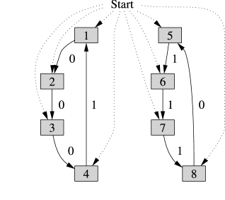
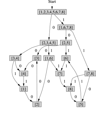
Figure 3: The domains $\mathcal{D}_{1}$ and $\mathcal{D}_{2}$ (top) and the automaton $\mathcal{A}=\mathrm{Det}(\mathcal{D}_{1}\sqcup\mathcal{D}_{2})$ (bottom). Start states are indicated by dotted arrows from the word “Start”, and final states are darkened. Notice that the states of $\mathcal{A}$ correspond to collections of states of $\mathcal{D}_{1}$ and $\mathcal{D}_{2}$ and that the former are canonically injected into the latter, here by the map $n\mapsto[n]$.

Let $\mathcal{T}$ be a transducer with the same states, start state, and final states as $\mathcal{A}$, but with the transitions:

$$T(\mathcal{T}):= \{(s,a|f(s^{\prime}),s^{\prime}):(s,a,s^{\prime})\in T(\mathcal{A})\}~{},$$

where:

$$f(s^{\prime})=\begin{cases}i&\text{if $\phi_{\mathcal{A}}(s^{\prime})\subset S(\mathcal{D}_{i})$}~{},\\ \lambda&\text{otherwise}~{},\end{cases}$$

and where $\lambda$ is a new symbol in the output alphabet $\Sigma^{\prime}$ indicating that domain labeling was not possible, for example, because the partial string read so far belongs to more than one or none of the automata $\{\mathcal{D}_{i}\}$. To recapitulate, the transducer’s output alphabet $\Sigma^{\prime}$ consists of three kinds of symbol: domain labels $\{1\ldots n\}$, domain-domain transition types $\{1,2,\ldots,p\}$, and ambiguity $\lambda$.

The transducer $\mathcal{T}$’s input, $\mathrm{In}(\mathcal{T})$, recognizes precisely those strings recognized by the given domains. Our goal is to extend $\mathcal{T}$ by introducing transitions of the form:

$$\{(s,a|h(s,a),g(s,a))\ :\ s\in S(\mathcal{T})=S(\mathcal{A}),a\in\Sigma,$$

and there are no transitions

$$\text{of the form $(s,a,\cdot)\in T(\mathcal{A})$}\}~{},$$

where the functions $g(s,a)$ and $h(s,a)$ are defined in the following paragraphs. The transducer $\mathrm{Filter}(\{\mathcal{D}_{i}\})$ obtained by adding these transitions to $\mathcal{T}$ will then have the desired property that its input $\mathrm{In}(\mathrm{Filter}(\{\mathcal{D}_{i}\}))$ will accept all strings .

Let $W_{l}$ denote the collection of strings corresponding to length-$l$ paths through $\mathcal{A}$ beginning in any of its states, but ending in state $s$, and let $W^{\prime}_{l+1}$ denote the collection of strings obtained by appending the letter $a$ to the strings of $W_{l}$. The strings $\bigcup_{l\geq 0}W^{\prime}_{l}$ are accepted by the finite automaton $\mathcal{A}^{s,a}$ obtained by adding a new state $f$ and a transition $(s,a,f)$ to $\mathcal{A}$, and by setting $\mathrm{Start}(\mathcal{A}^{s,a}):=S(\mathcal{A}^{s,a})$ and $\mathrm{Final}(\mathcal{A}^{s,a}):=\{f\}$. An example is shown in Fig. 4, where the four-state domain has a transition added from state [2] on symbol $1$, which was originally forbidden.

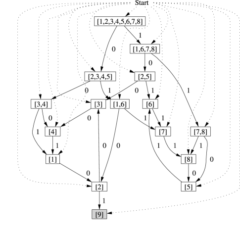
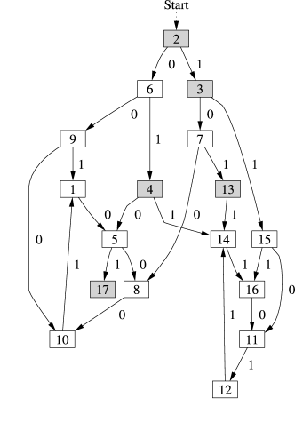
Figure 4: The semi-deterministic automaton $\mathcal{A}^{[2],1}$ (top) obtained by adding a state $f=[9]$ and its deterministic version $\mathrm{Det}(\mathcal{A}^{[2],1})$ (bottom) with states relabeled with the integers $1\dots 17$ in order to simplify later diagrams.

In order to choose the resynchronization state $g(s,a)$ for the forbidden transition $(s,a)$, we examine the strings of $\bigcup_{l\geq 0}W^{\prime}_{l}$ that also belong to one or more of the domains $\{\mathcal{D}_{i}\}$. We do this by constructing the automaton $\mathrm{Det}(\mathcal{A}^{s,a})\cap\mathcal{A}$, which we call the resynchronization automaton. By Lemma 3, there is a canonical, although not necessarily injective, association:

$$\phi:S(\mathrm{Det}(\mathcal{A}^{s,a})\cap\mathcal{A})\rightarrow S(\mathcal{A})$$

given by the composition:

$$S(\mathrm{Det}(\mathcal{A}^{s,a})\cap\mathcal{A})\ \ \hookrightarrow\ \ S(\mathrm{Det}(\mathcal{A}^{s,a}))\times S(\mathcal{A})\ \ \rightarrow\ \ S(\mathcal{A})~{},$$

where the right-most map is the second-factor projection, $(s,s^{\prime})\mapsto s^{\prime}$.

The resynchronization automaton $\mathrm{Det}(\mathcal{A}^{s,a})\cap\mathcal{A}$ may reveal several possible resynchronization states. To help distinguish among them, we put them into sets $\{S_{i,l}\}$ where $i$ measures the specificity of resynchronization and $l$ the length of imagined past. More precisely, let $S_{i,l}$ denote those states $s\in S(\mathcal{A})$ to which $\phi$ associates at least one state $s^{\prime}\in\mathrm{Final}(\mathrm{Det}(\mathcal{A}^{s,a})\cap\mathcal{A})$ (i.e. $s=\phi(s^{\prime})$) satisfying the following two conditions: (1) $s$ corresponds, under Lemma 2, to precisely $i$ states of $\mathcal{D}_{1}\sqcup\cdots\sqcup\mathcal{D}_{n}$ and (2) there is a length-$l$ path from the unique start state of $\mathrm{Det}(\mathcal{A}^{s,a})\cap\mathcal{A}$ to $s^{\prime}$.

Give the sets $\{S_{i,l}\}$ the dictionary ordering; that is, let $S_{i,l}<S_{i^{\prime},l^{\prime}}$ if $i<i^{\prime}$ or if $i=i^{\prime}\wedge l<l^{\prime}$. The set $S_{|S(\mathcal{A})|,0}$ consists of the unique start state of $\mathrm{Det}(\mathcal{A}^{s,a})\cap\mathcal{A}$. Thus, by the well ordering principle, there must be a unique, least set among the sets $\{S_{i,l}\}$ that consist of a single state, say $\{s^{\prime}\}$. Let $g(s,a):=s^{\prime}$, and let $h(s,a):=h^{\prime}(s,s^{\prime})=h^{\prime}(s,g(s,a))$, where $h^{\prime}$ is any injection $S(\mathcal{T})\times S(\mathcal{T})\hookrightarrow\Sigma^{\prime}$ (chosen independent of $s$ and $a$). An example of this construction is shown in Fig. 5.

The transducer is completed by repeating the above steps for all forbidden transitions.

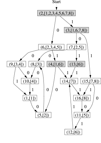
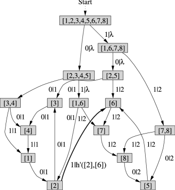
Figure 5: The resynchronization automaton $\mathrm{Det}(\mathcal{A}^{[2],1})\cap\mathcal{A}$ (top). Here $S_{1,3}$ consists of the state $(13,[6])$ alone, and all other $S_{1,\bullet}$ are empty. So we choose $s^{\prime}=[6]$ and add a transition $([2],1|h^{\prime}([2],[6]),[6])$ to $\mathcal{T}$ (bottom).

Computability of the transducer $\mathrm{Filter}(\{\mathcal{D}_{i}\})$

Although the transducer $\mathrm{Filter}(\{\mathcal{D}_{i}\})$ is well defined, it is perhaps not immediately clear that it is computable. After all, we appealed to the well ordering principle to obtain a least singleton set $\{s^{\prime}\}$ among the sets $\{S_{i,l}\}$. In fact, infinitely many sets $S_{i,l}$ precede the stated upper bound $S_{|S(\mathcal{A})|,0}$—for instance, all of the sets $S_{1,\mathbb{N}}$ do, provided $|S(\mathcal{A})|>1$.

The construction is nevertheless computable, because for each $i$ the sequence of sets $S_{i,\mathbb{N}}$ must eventually repeat. In fact, we can compute this sequence of sets exactly by automata-theoretic means.

Proposition 4.

The transducer $\mathrm{Filter}(\{\mathcal{D}_{i}\})$ is computable.

Proof.

Let $\mathcal{Z}[\mathcal{C}]$ denote the automaton obtained by relabeling all of the automaton $\mathcal{C}$’s transitions with $0$s. This automaton will almost certainly be nondeterministic. The equivalent deterministic automaton $\mathrm{Det}(\mathcal{Z}[\mathcal{C}])$ is useful, because the state it reaches when accepting the string $0^{l}$ corresponds precisely, under Lemma 2, to the collection of states that can be reached by length-$l$ paths through $\mathcal{C}$.

Moreover, since $\mathrm{Det}(\mathcal{Z}[\mathcal{C}])$ is defined over a single letter, yet deterministic and finite, it must have a special graphical structure: its single start state $s_{0}$ must lead to a finite loop after a finite chain of non-recurrent states. (Actually, if $\mathcal{C}$ has no loops whatsoever, there will not even be a loop.) Thus, its states have a linear ordering: $s_{0}\stackrel{{\scriptstyle 0}}{{\rightarrow}}s_{1}\stackrel{{\scriptstyle 0}}{{\rightarrow}}\cdots\stackrel{{\scriptstyle 0}}{{\rightarrow}}s_{m}\stackrel{{\scriptstyle 0}}{{\rightarrow}}s_{m+1}\stackrel{{\scriptstyle 0}}{{\rightarrow}}\cdots\stackrel{{\scriptstyle 0}}{{\rightarrow}}s_{m+m^{\prime}}\stackrel{{\scriptstyle 0}}{{\rightarrow}}s_{m}$. An example is illustrated in Fig. 6, where $m=4$ and $m^{\prime}=0$.

By Lemma 2 the states $\{s_{k}\}$ correspond to collections of states of $\mathcal{C}$ under an injection:

$$\psi_{\mathcal{Z}[\mathcal{C}]}:S(\mathrm{Det}(\mathcal{Z}[\mathcal{C}]))\hookrightarrow \{S\subset S(\mathcal{Z}[\mathcal{C}])\}$$

$$= \{S\subset S(\mathcal{C})\}.$$

Let $\mathcal{C}:=\mathrm{Det}(\mathcal{A}^{s,a})\cap\mathcal{A}$ in the preceding discussion. As before, by Lemma 3, there is a function:

$$\phi:S(\mathrm{Det}(\mathcal{A}^{s,a})\cap\mathcal{A})\rightarrow S(\mathcal{A})~{}.$$

Let $S_{*,l}\subset S(\mathcal{A})$ denote those states defined by the formula:

$$S_{*,l}:=\phi[\psi_{\mathcal{Z}[\mathcal{C}]}(s_{l})\cap\mathrm{Final}(\mathrm{Det}(\mathcal{A}^{s,a})\cap\mathcal{A})]~{}.$$

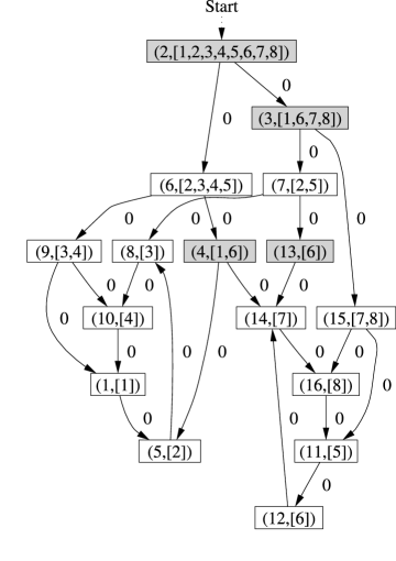
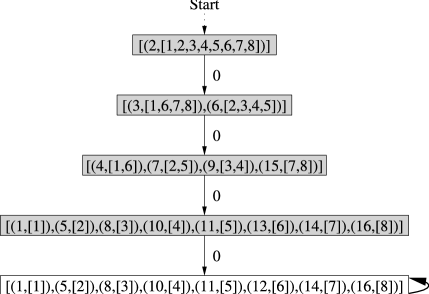
Figure 6: The automaton $\mathcal{Z}[\mathrm{Det}(\mathcal{D}_{1}^{[2],1})\cap\mathcal{A}]$ (top) and its deterministic version $\mathrm{Det}(\mathcal{Z}[\mathrm{Det}(\mathcal{D}_{1}^{[2],1})\cap\mathcal{A}])$ (bottom).

Finally, let $S_{i,*}$ denote those states of $\mathcal{A}$ that correspond to precisely $i$ states of $\mathcal{D}_{1}\sqcup\cdots\sqcup\mathcal{D}_{n}$; that is, let:

$$S_{i,*}:=\{s\in S(\mathcal{A}):|\phi_{\mathcal{A}}(s)|=i\}~{},$$

where $\phi_{\mathcal{A}}:S(\mathcal{A})\hookrightarrow\{S\subset S(\mathcal{D}_{1}\sqcup\cdots\sqcup\mathcal{D}_{n})\}$ is the injection provided by Lemma 2.

The sets $S_{i,l}$ can then be computed as the intersections $S_{i,*}\cap S_{*,l}$, and we need only examine these for $1\leq i\leq|S(\mathcal{D}_{1})|+\dots+|S(\mathcal{D}_{n})|$ and $0\leq l\leq m+m^{\prime}$ to discover the least one under the dictionary ordering that is a singleton $\{s^{\prime}\}$. ∎

We summarize the entire algorithm.

Algorithm 2.

Input: The regular domains $\mathcal{D}_{1},\dots,\mathcal{D}_{n}$.

• Let $\mathcal{A}:=\mathrm{Det}(\mathcal{D}_{1}\sqcup\cdots\sqcup\mathcal{D}_{n})$.

• Choose any injection $h^{\prime}:S(\mathcal{A})\times S(\mathcal{A})\hookrightarrow\Sigma^{\prime}$.

• Make $\mathcal{A}$ into a transducer $\mathcal{T}$ by adding the symbol $i$ as output to any transition ending in a state corresponding to states of only one domain $\mathcal{D}_{i}$ and by adding $\lambda$s as output symbols to all other transitions.

• For each forbidden transition $(s,a)\in S(\mathcal{A})\times\Sigma(\mathcal{A})$, add a transition to $\mathcal{T}$ through the following procedure do

  • Construct the automaton $\mathcal{A}^{s,a}$ by adding to $\mathcal{A}$ the transition $(s,a,f)$, where $f$ is a new state, and by letting $f$ be its only final state.

  • Construct the automaton $\mathrm{Det}(\mathcal{Z}[\mathrm{Det}(\mathcal{A}^{s,a})\cap\mathcal{A}])$, where $\mathcal{Z}[\mathcal{C}]$ is the automaton obtained by relabeling all of $\mathcal{C}$’s transitions with $0$s. Its states will have a natural linear ordering $s_{0}\rightarrow s_{1}\rightarrow\cdots\rightarrow s_{m+m^{\prime}}.$

  • Let $S_{i,*}$ and $S_{*,l}$ be the subsets of $S(\mathcal{A})$ defined by:

    $$S_{*,l} :=\phi[\psi_{\mathrm{Det}(\mathcal{Z}[\mathrm{Det}(\mathcal{A}^{s,a})\cap\mathcal{A}])}(s_{l})$$

    $$\;\;\;\;\;\;\;\;\;\;\cap\mathrm{Final}(\mathrm{Det}(\mathcal{A}^{s,a})\cap\mathcal{A})]\text{\ and}$$

    $$S_{i,*} :=\{s\in S(\mathcal{A}):|\psi_{\mathcal{A}}(s)|=i\}.$$

  • Find the singleton set $\{s^{\prime}\}$ among the sets:

    $$\{S_{i,*}\cap S_{*,l}:\; 1\leq i\leq|\mathcal{D}_{1}|+\cdots+|\mathcal{D}_{n}|,$$

    $$0\leq l\leq m+m^{\prime}\}$$

    that occurs first under the dictionary ordering.

  • Add the transition $(s,a|h^{\prime}(s,s^{\prime}),s^{\prime})$ to $\mathcal{T}$.

Output: $\mathrm{Filter}(\{\mathcal{D}_{i}\}):=\mathcal{T}$.

Algorithmic Complexity

Proposition 5.

The worst-case performance of the transducer-constructing algorithm (Algorithm 2) has order no greater than:

$$|\mathcal{A}|\cdot(|\Sigma|-1)\cdot\exp\circ\exp\left(2\cdot|\mathcal{A}|+1\right)~{},$$

where $|\mathcal{A}|$ has order $\exp(|\mathcal{D}_{1}|+\cdots+|\mathcal{D}_{n}|)$.

Proof.

The algorithm’s most expensive step is the computation of $\mathrm{Det}(\mathcal{Z}[\mathrm{Det}(\mathcal{A}^{s,a})\cap\mathcal{A}])$. Unfortunately, because computing $\mathrm{Det}(\mathcal{G})$ has order $\mathrm{exp}(|\mathcal{G}|)$, and because computing $\mathcal{G}\cap\mathcal{H}$ has order $|\mathcal{G}|\cdot|\mathcal{H}|$, this computation has order $\exp\circ\exp\left(2\cdot|\mathcal{A}|+1\right)$.

Finally, recall that the algorithm computes $\mathrm{Det}(\mathcal{Z}[\mathrm{Det}(\mathcal{A}^{s,a})\cap\mathcal{A}])$ for every forbidden transition $(s,a)$ of $\mathcal{A}$. A rough upper bound for the number of such transitions is $|\mathcal{A}|\cdot(|\Sigma|-1)$. From these two upper bounds the proposition follows. ∎

Although this analysis may at first seem to objurgate the transducer-constructing algorithm, the reader should realize that, once computed, $\mathcal{T}$ can be very efficiently used to filter arbitrarily long strings. That is, unlike the stack-based algorithm, its performance is linear in string length. Thus, one pays during the filter design phase for an efficient run-time algorithm—a trade-off familiar, for example, in data compression.

Constructing optimal transducers from non-minimal domains, a preprocessing step to Algorithm 2

Recall that we constructed the transducer $\mathrm{Filter}(\{\mathcal{D}_{i}\})$ by ‘filling in’ the forbidden transitions of the automaton $\mathcal{A}:=\mathrm{Det}(\mathcal{D}_{1}\sqcup\dots\sqcup\mathcal{D}_{n})$. This proved somewhat problematic, however, because $\mathcal{A}$’s states do not always preserve enough information about past input to unambiguously resynchronize to a unique, recurrent domain state. In order to help discriminate among the several possible resynchronization states, we introduced the partially ordered sets $\{S_{i,l}\}$. But even so, several attractive resynchronization states often fell into the same set $S_{i,l}$. So, lacking any objective way to choose among them, we resigned ourselves to a less attractive resynchronization state occurring in a later set $S_{i^{\prime},l^{\prime}}$, simply because it appeared alone there, making our choice unambiguous. If only the states of the automaton $\mathcal{A}$ preserved slightly more information about past input, then such compromises could be avoided.

In this section we present an algorithm that splits the states of a given collection $\{\mathcal{D}_{i}\}$ of domains to obtain an equivalent collection $\{\mathcal{D}^{\prime}_{i}\}=\mathrm{Optimize}(\{\mathcal{D}_{i}\})$ of domains that preserve just enough information about past input to enable unambiguous resynchronization in the transducer obtained by filling in the forbidden transitions of the automaton $\mathcal{A}^{\prime}:=\mathrm{Det}(\mathcal{D}^{\prime}_{1}\sqcup\dots\sqcup\mathcal{D}^{\prime}_{n})$.

We will accomplish this by associating to each state of the original domains $\mathcal{D}_{i}$ a collection of automata that partition past input strings into equivalence classes corresponding to individual resynchronization states. We will then refine these partitions so that $\mathcal{D}_{i}$’s transition structures can be lifted to them and thus obtain the desired domains $\{\mathcal{D}^{\prime}_{i}\}=\mathrm{Optimize}(\{\mathcal{D}_{i}\})$.

This procedure, taken as a preprocessing step to Algorithm 2, will thus produce the best possible transducer for Method-2 multi-regular language filtering.

We now state our construction formally. If $s^{\prime}\in S(\mathcal{A})$, then let $\mathcal{A}_{s^{\prime}}$ denote the automaton that is identical to the automaton $\mathcal{A}$ except that its only final state is $s^{\prime}$. Additionally, if $(s,a)$ is a forbidden transition of the automaton $\mathcal{D}_{1}\sqcup\dots\sqcup\mathcal{D}_{n}$, then let $\mathcal{B}(s,a,s^{\prime})$ denote the automaton satisfying the formula:

$$\mathcal{B}(s,a,s^{\prime})\cdot a=\mathrm{Det}(\mathcal{A}^{s,a})\cap\mathcal{A}_{s^{\prime}}~{},$$

where $\cdot$ denotes concatenation. That is, let $\mathcal{B}(s,a,s^{\prime})$ denote the automaton that is identical to the automaton $\mathrm{Det}(\mathcal{A}^{s,a})\cap\mathcal{A}_{s^{\prime}}$ except that its final states are given by $\{s_{f}:(s_{f},a,s_{f}^{\prime})\in T(\diamond),s_{f}^{\prime}\in\mathrm{Final}(\diamond)\}$, where $\diamond:=\mathrm{Det}(\mathcal{A}^{s,a})\cap\mathcal{A}_{s^{\prime}}$. Note that in most cases $\mathrm{Lang}(\mathcal{B}(s,a,s^{\prime}))$ will be empty.

Next we associate to each state $s\in S(\mathcal{D}_{1}\sqcup\dots\sqcup\mathcal{D}_{n})$ a collection $\Gamma(s)$ of automata. If the state $s$ has no forbidden transitions, let $\Gamma(s):=\{\Sigma^{*}\}$. If the state $s$ has at least one forbidden transition, however, then let $\Gamma(s)$ denote the collection of automata:

$$\Gamma(s):=\mathrm{Disjoin}(\{ \Sigma^{*}\cdot\mathcal{B}(s,a,s^{\prime}):$$

$$(s,a,\cdot)\not\in T(\mathcal{A}),s^{\prime}\in S(\mathcal{A})\})~{},$$

where $\mathrm{Disjoin}(\{\mathcal{C}_{\gamma}\})$ denotes the coarsest partition of $\bigcup_{\gamma}\mathrm{Lang}(\mathcal{C}_{\gamma})$ by automata $\{\mathcal{E}_{\epsilon}\}$ that is compatible with the automata $\{\mathcal{C}_{\gamma}\}$. That is, $\mathrm{Disjoin}(\{\mathcal{C}_{\gamma}\})$ denotes the smallest collection $\{\mathcal{E}_{\epsilon}\}$ of automata satisfying (i) $\bigcup_{\epsilon}\mathrm{Lang}(\mathcal{E}_{\epsilon})=\bigcup_{\gamma}\mathrm{Lang}(C_{\gamma})$ and (ii) $\mathrm{Lang}(\mathcal{C}_{\gamma})\cap\mathrm{Lang}(\mathcal{E}_{\epsilon})$ is either empty or equal to $\mathrm{Lang}(\mathcal{E}_{\epsilon})$ for all $\gamma$ and $\epsilon$.

It is possible to compute $\mathrm{Disjoin}(\{\mathcal{C}_{\gamma}\})$ inductively with the formula:

$$\mathrm{Disjoin} (\{\mathcal{C}_{1},\mathcal{C}_{2},\dots,\mathcal{C}_{m}\})=$$

$$\{\mathcal{C}_{1}\setminus(\mathcal{C}_{2}\sqcup\cdots\sqcup\mathcal{C}_{m})\}\;\cup$$

$$\{\mathcal{C}_{1}\cap\mathcal{C}^{\prime}:\mathcal{C}^{\prime}\in\mathrm{Disjoin}(\{\mathcal{C}_{2},\dots,\mathcal{C}_{m}\})\}\;\cup$$

$$\{\mathcal{C}_{1}\setminus\mathcal{C}^{\prime}\,:\mathcal{C}^{\prime}\in\mathrm{Disjoin}(\{\mathcal{C}_{2},\dots,\mathcal{C}_{m}\})\}.$$

Note that $\bigcup_{\mathcal{E}\in\Gamma(s)}\mathrm{Lang}(\mathcal{E})=\Sigma^{*}$ for all states $s\in S(\mathcal{D}_{1}\sqcup\dots\sqcup\mathcal{D}_{n})$. This is because $\mathrm{Lang}(\mathcal{B}(s,a,s^{\prime}))$ contains only the empty string if $s^{\prime}\in S(\mathcal{A})$ is the unique state reached on input $a$ from $\mathcal{A}$’s starting state—that is, if $(s_{0},a,s^{\prime})\in T(\mathcal{A})$, where $\{s_{0}\}=\mathrm{Start}(\mathcal{A})$.

Our goal is to create for each original domain $\mathcal{D}_{i}$ an equivalent domain $\mathcal{D}^{\prime}_{i}$ by splitting each state $s\in S(\mathcal{D}_{i})$ into states of the form $(s,\mathcal{E})$, where $\mathcal{E}\in\Gamma(s)$. But to endow these split states with a transition structure equivalent to $\mathcal{D}_{i}$’s, we typically must refine the sets $\Gamma(s)$ further. We must construct a refinement $\Gamma^{\prime}(s)$ of each $\Gamma(s)$ with the property that if $(s,a,s^{\prime})$ is a transition of $\mathcal{D}_{i}$, then to each $\mathcal{E}\in\Gamma^{\prime}(s)$ there corresponds a unique $\mathcal{E}^{\prime}\in\Gamma^{\prime}(s^{\prime})$ with $\mathrm{Lang}(\mathcal{E}\cdot a)\subset\mathrm{Lang}(\mathcal{E}^{\prime})$. Given such refinements $\Gamma^{\prime}(s)$, we can take the pairs $\{(s,\mathcal{E}):s\in S(\mathcal{D}_{i}),\mathcal{E}\in\Gamma^{\prime}(s)\}$ as the states of $\mathcal{D}^{\prime}_{i}$ and equip them with transitions of the form $(s,\mathcal{E})\stackrel{{\scriptstyle a}}{{\rightarrow}}(s^{\prime},\mathcal{E}^{\prime})$, and thus obtain an equivalent, but non-minimal, domain $\mathcal{D}^{\prime}_{i}$.

The following algorithm can be used to compute the desired refinements $\Gamma^{\prime}(s)$.

Algorithm 3.

Input: The domain $\mathcal{D}$ and the function $\Gamma$ that assigns to each state $s\in S(\mathcal{D})$ a collection $\Gamma(s)$ of automata that partition $\Sigma^{*}$.

• For each state $s\in S(\mathcal{D})$, let:

  $$\Gamma^{\prime}(s) :=\mathrm{Disjoin}\left(\bigcup\{\Gamma^{\prime}(s,a,s^{\prime}):(s,a,s^{\prime})\in T(\mathcal{D})\}\right)~{},$$

  where:

  $$\Gamma^{\prime}(s,a,s^{\prime}) :=\{\mathcal{E}_{\alpha}^{\prime\prime}\}_{\alpha}\text{\ and}$$

  $$\{\mathcal{E}_{\alpha}^{\prime\prime}\cdot a\}_{\alpha} :=\{(\mathcal{E}\cdot a)\cap\mathcal{E}^{\prime}:\mathcal{E}\in\Gamma(s),\mathcal{E}^{\prime}\in\Gamma(s^{\prime})\}.$$

• If $\Gamma^{\prime}(s)\neq\Gamma(s)$ for some state $s\in S(\mathcal{D})$, then repeat with $\Gamma^{\prime}$ in place of $\Gamma$. Otherwise:
  

Output: $\Gamma^{\prime}$.

Proposition 6.

Algorithm 3 eventually terminates, producing the coarsest possible refinements $\Gamma^{\prime}(s)$ of $\Gamma(s)$ compatible with $\mathcal{D}$’s transition structure.

Proof.

We construct fine, but finite, refinements that are compatible with $\mathcal{D}$’s transition structure, then use this result to conclude that Algorithm 3 must eventually terminate. Moreover, we also conclude that, when Algorithm 3 terminates, it produces the coarsest possible refinements that are compatible with $\mathcal{D}$’s transition structure.

Let $\{\mathcal{E}_{i}\}$ denote the potentially large, but finite, collection of automata:

$$\{\mathcal{E}_{i}\}_{i=1}^{N}:=\mathrm{Disjoin}\left(\bigcup_{s\in S(\mathcal{D})}\!\!\!\Gamma(s)\right)~{},$$

which partition $\Sigma^{*}$.

We refine the partition $\{\mathcal{E}_{i}\}$ to make it compatible with $\mathcal{D}$’s transitions by examining the automaton $\mathcal{F}:=\mathrm{Det}(\mathcal{E}_{1}\sqcup\dots\sqcup\mathcal{E}_{N})$. Since the automata $\{\mathcal{E}_{i}\}$ cover $\Sigma^{*}$, the deterministic automaton $\mathcal{F}$ can have no forbidden transitions, and all its states must be final. Moreover, because the automata $\{\mathcal{E}_{i}\}$ are disjoint, each of $\mathcal{F}$’s states must correspond (under the canonical injection $\psi_{\mathcal{F}}$ of Lemma 2) to final states of precisely one automaton $\mathcal{E}_{i}$. In this way, the automata $\{\mathcal{E}_{i}\}$ correspond to a partition of the states of $\mathcal{F}$.

Since each automaton $\mathcal{E}_{i}$ is equivalent to the automaton obtained by restricting $\mathcal{F}$’s final states to those states corresponding (under $\psi_{\mathcal{F}}$) to final states of $\mathcal{E}_{i}$, we can refine the partition $\{\mathcal{E}_{i}\}$ by refining this partition of $\mathcal{F}$’s states.

Although a coarser refinement may suffice, we can always choose the partition consisting of single states. That is, if $s\in S(\mathcal{F})$, let $\mathcal{F}_{s}$ denote the automaton that is identical to the automaton $\mathcal{F}$ except that its only final state is $s$. Then $\{\mathcal{F}_{s}:s\in S(\mathcal{F})\}$ is a refinement of the partition $\{\mathcal{E}_{i}\}$ with the special property that for each automaton $\mathcal{F}_{s}$ and $a\in\Sigma(\mathcal{F})$, there is a unique automaton $\mathcal{F}_{s^{\prime}}$ such that $\mathcal{F}_{s}\cdot a=\mathcal{F}_{s^{\prime}}$. Indeed, since $\mathcal{F}$ is deterministic, $s^{\prime}$ is the unique state corresponding to a transition $(s,a,s^{\prime})\in T(\mathcal{F})$.

If we let $\Gamma^{\prime\prime}(s):=\{\mathcal{F}_{s^{\prime}}:s^{\prime}\in S(\mathcal{F})\}$ for each state $s\in S(\mathcal{D})$, then we obtain finite refinements of $\Gamma(s)$ compatible with $\mathcal{D}$’s transition structure, as desired.

This result implies that Algorithm 3 must eventually terminate. After all, every refinement that Algorithm 3 performs must already be reflected in $\Gamma^{\prime\prime}(s)$. Moreover, since every refinement that the algorithm performs is essential to compatibility with $\mathcal{D}$’s transition structure, the algorithm must, upon termination, produce the coarsest (smallest) compatible refinement possible. ∎

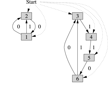
Figure 7: The positive-entropy domains $\mathcal{D}_{1}$ and $\mathcal{D}_{2}$ of the binary, next-to-nearest neighbor ca 2614700074. (After Ref. Crut93a .)

When applied to the domains $\mathcal{D}_{1}$ and $\mathcal{D}_{2}$ in Fig. 7, for example, Algorithm 3 produces the equivalent, non-minimal domains $\{\mathcal{D}^{\prime}_{1},\mathcal{D}^{\prime}_{2}\}=\mathrm{Optimize}(\{\mathcal{D}_{1},\mathcal{D}_{2}\})$ shown in Fig. 8. Notice these domains’ many non-recurrent states. These have almost no effect on the automaton $\mathcal{A}^{\prime}:=\mathrm{Det}(\bigsqcup_{i}\mathcal{D}^{\prime}_{i})$.

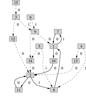
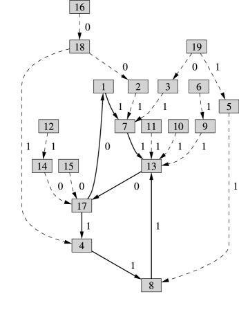
Figure 8: The equivalent, non-minimal domains $\{\mathcal{D}^{\prime}_{1},\mathcal{D}^{\prime}_{2}\}=\mathrm{Optimize}(\{\mathcal{D}_{1},\mathcal{D}_{2}\})$ obtained by applying Algorithm 3 to the positive-entropy domains $\mathcal{D}_{1}$ and $\mathcal{D}_{2}$ in Fig. 7. ($\mathcal{D}^{\prime}_{1}$ (top) and $\mathcal{D}^{\prime}_{2}$ (bottom).) The “Start” arrows are omitted for clarity (all states are starting), and some of the transitions are drawn with dashed arrows to help the reader distinguish the recurrent states.

IV Applications

We now present four applications to illustrate how the stack-based Algorithm 1 and its transducer approximation (Algorithms 2 and 3) solve the multi-regular language filtering problem. The first is the cellular automaton eca 110, shown previously. Its rather large filtering transducer is quite tedious to construct by hand, but Algorithm 2 produces it handily. The second example, eca 18, which we have also already seen, illustrates the stack-based Algorithm 1’s ability to detect overlapping domains. The third example shows our methods’ power to detect structures in the midst of apparent randomness: the domains and sharp boundaries between them are identified easily despite the fact that the domains themselves have positive entropy and their boundaries move stochastically. The example shows the use of—and need for—domain-preprocessing (Algorithm 3). That is, rapid resynchronization is achieved using a filter built from optimized, non-minimal domains. The final example demonstrates the transducer (constructed by Algorithms 2 and 3) detecting domains in a multi-stationary process—what is called the change-point problem in statistical time-series analysis. This example emphasizes that the methods developed here are not limited to cellular automata. More importantly, it highlights several of the subtleties of multi-regular language filtering and clearly illustrates the need for the domain-preprocessing Algorithm 3.

Eca 110

First consider eca 110, illustrated earlier in Fig. 1. Its domains are easy to see visually; they have the form $\mathrm{sub}(w^{*})$ for some finite word $w$. Its dominant domain is $\mathrm{sub}(w^{*})=\mathrm{sub}[(00010011011111)^{*}]$, illustrated in Fig. 9.

Figure 9: eca 110’s principal domain, $\mathrm{sub}[(00010011011111)^{*}]$.

In fact, the transducer $\mathrm{Filter}(\{\mathrm{sub}[(00010011011111)^{*}]\})$, constructed from this single domain, filters eca 110’s space-time behavior well; see Fig. 10.

Notice, in that figure, the wide variety of particle-like domain defects that the filtered version lays bare. Note, moreover, how these particles move and collide according to consistent rules. These particles are important to eca 110’s computational properties; a subset can be used to implement a Post Tag system Mins67 and thus simulate arbitrary Turing machines Cook04 .

Figure 10: An eca 110 space-time diagram (left) filtered by the transducer $\mathrm{Filter}(\{\mathrm{sub}[(00010011011111)^{*}]\})$ (right).

Eca 18

Next, consider Eca 18, illustrated earlier in Fig. 2. It is somewhat more challenging to filter, because its domain $\mathcal{D}=\mathrm{sub}\left([0(0+1)]^{*}\right)$ has positive entropy. As a result, its particles are difficult—although by no means impossible—to see with the naked eye. Nevertheless, the stack-based algorithm filters its space-time diagrams extremely well, as illustrated in Fig. 2 (right). There, black rectangles are drawn where maximal substrings overlap, and vertical bars are drawn where maximal substrings abut. As mentioned earlier, these particles, whose precise location is somewhat ambiguous, follow random walks and pairwise annihilate whenever they touch Crut92a ; Eloranta94 ; Hans90a .

It is worth mentioning that the transducer $\mathrm{Filter}(\{\mathcal{D}\})$ produces a less precise filtrate in this case—and that $\mathrm{Filter}(\mathrm{Optimize}(\{\mathcal{D}\}))$ does no better. Indeed, since breaks in eca 18’s domain have the form $\cdots 1(0^{2n})1\cdots$, the precise location of the domain break is ambiguous: if reading left-to-right, it does not occur until the $1$ on the right of $0^{2n}$ is read; whereas, if reading right-to-left, it does not occur until the $1$ on the left is read. In other words, if reading left-to-right, the transducer $\mathrm{Filter}(\{\mathcal{D}\})$ detects only the right edges of the black triangles of Fig. 2 (right). Similarly, if reading right-to-left, it detects only the left edges of these triangles. In this case it is possible to fill in the space between these pairs of edges to obtain the output of the stack-based algorithm.

Ca 2614700074

Now consider the binary, next-to-nearest neighbor (i.e. $k$=$r$=2) ca 2614700074, shown in Fig. 11. Crutchfield and Hanson constructed it expressly to have the positive-entropy domains $\mathcal{D}_{1}$ and $\mathcal{D}_{2}$ in Fig. 7 Crut93a .

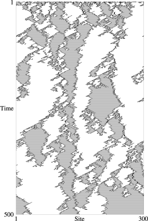
Figure 11: Binary, next-to-nearest neighbor ca 2614700074 space-time diagram (left) filtered by the transducer $\mathrm{Filter}(\mathrm{Optimize}(\{\mathcal{D}_{1},\mathcal{D}_{2}\}))$ (right). The white regions on the right correspond to the domain $\mathcal{D}_{1}$, the gray to the domain $\mathcal{D}_{2}$. The black squares separating these regions correspond to the interruption symbols $h^{\prime}(s,s^{\prime})$ that the transducer emits between domains.

As illustrated in Fig. 11, the optimal transducer $\mathrm{Filter}(\mathrm{Optimize}(\{\mathcal{D}_{1},\mathcal{D}_{2}\}))$ filters this ca’s output well. This illustrates a practical advantage of multi-regular language filtering: it can detect structure embedded in randomness. Notice how the filter easily identifies the domains and sharp boundaries separating them, even though the domains themselves have positive entropy and their boundaries move stochastically.

It is worth noting that in place of the gray regions of Fig. 11 so clearly identified by the optimal transducer as corresponding to the second domain $\mathcal{D}_{2}$, the simpler transducer $\mathrm{Filter}(\{\mathcal{D}_{1},\mathcal{D}_{2}\})$ produces a regular checkering of false domain breaks (not pictured). This is because, when examining the sole forbidden transition $(s,a)=(2,1)$ of the first domain $\mathcal{D}_{1}$, Algorithm 2 discovers that the first non-empty set $S_{i=1,l=4}=\{2,4,5\}$ contains three resynchronization states. It unfortunately abandons both states 4 and 5, which belong to the second domain, instead choosing to resynchronize to the original state 2 itself, because it occurs alone in the next set $S_{1,5}$. As a result, the transducer $\mathrm{Filter}(\{\mathcal{D}_{1},\mathcal{D}_{2}\})$ has no transitions leaving the first domain whatsoever and is therefore incapable of detecting jumps from the first domain to the second. This is why it prints a checkering of domain breaks instead of correctly resynchronizing to the second domain. The optimal transducer does not suffer from this problem, because Algorithm 3 splits state 2 into several new ones, from which unambiguous resynchronization to the appropriate state—2, 4, or 5—is possible.

Change-Point Problem: Filtering Multi-Stationary Sources

Leaving cellular automata behind, consider a binary information source that hops with low probability between the two three-state domains $\mathcal{D}_{1}$ and $\mathcal{D}_{2}$ in Fig. 12 (top). This source allows us to illustrate subtleties in multi-regular language filtering and, in particular, in the construction of the optimal transducer $\mathrm{Filter}(\mathrm{Optimize}(\{\mathcal{D}_{i}\})$ can be.

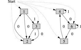
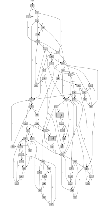
Figure 12: Two similar three-state domains $\mathcal{D}_{1}$ (top left) and $\mathcal{D}_{2}$ (top right) illustrate how subtle the construction of the optimal transducer $\mathrm{Filter}(\mathrm{Optimize}(\{\mathcal{D}_{i}\}))$ can be: the automaton $\mathcal{A}^{\prime}:=\mathrm{Det}(\bigsqcup\mathrm{Optimize}(\{\mathcal{D}_{1},\mathcal{D}_{2}\}))$ (below), from which the optimal transducer is constructed, has 69 states—the unoptimized automaton $\mathcal{A}:=\mathrm{Det}(\mathcal{D}_{1}\sqcup\mathcal{D}_{2})$ (not pictured) has 30.

To appreciate how subtle filtering with the domains $\mathcal{D}_{1}$ and $\mathcal{D}_{2}$ is—and why the extra states of $\mathrm{Optimize}(\{\mathcal{D}_{1},\mathcal{D}_{2}\})$ are needed to do it—consider the following. First choose any finite word $w$ of the form:

$$(0^{6}+0^{3}1^{2})^{*}0^{3}1^{2}0.$$

As the ambitious reader can verify, both of the strings $101111w$ and $110w$ belong to the domain $\mathcal{D}_{2}$. In fact, both correspond to unique paths through $\mathcal{D}_{1}\sqcup\mathcal{D}_{2}$ ending in state 5 of Fig. 12 (top).

On the other hand, the strings $01111w1$ and $10w1$ are also domain words—the first belonging to $\mathcal{D}_{2}$, but the second belonging to $\mathcal{D}_{1}$. In fact, $01111w1$ corresponds to a unique path through $\mathcal{D}_{1}\sqcup\mathcal{D}_{2}$ ending in state 6, while $10w1$ corresponds to a unique path ending in state 3.

As a result, these four strings are the maximal substrings of the non-domain strings $101111w1$ and $110w1$, as indicated by the brackets below:

corresponds to a unique path through $$\mathcal{D}_{2} {}1\;{} {}0\;1\;1\;1\;1\;w{} {}\;1{} \mathcal{D}_{2}$$ ending in state 5 corresponds to a unique path through ending in state 6

corresponds to a unique path through $$\mathcal{D}_{2} {}1\;{} {}1\;0\;w{} {}\;1{} \mathcal{D}_{1}$$ ending in state 5 corresponds to a unique path through ending in state 3

This example illustrates several important points. First of all, it shows that when the naive transducer $\mathrm{Filter}(\{\mathcal{D}_{1},\mathcal{D}_{2}\})$ reaches the forbidden letter 1 at the end of either of these two strings, the state 2 reached does not preserve enough information to resynchronize to the appropriate state—3 or 6, respectively. As a result, it must either make a guess—at the risk of choosing incorrectly and then later reporting an artificial domain break (as in the preceding cellular automaton example)—or else jump to one of its non-recurrent states, emitting a potentially long chain of $\lambda$s until it can re-infer from future input what was already determined by past input.

As unsettling as this may be, the example illustrates something far more nefarious. Since an arbitrarily long word $w$ can be chosen, it is impossible to fix the problem by splitting the states of $\mathrm{Filter}(\{\mathcal{D}_{1},\mathcal{D}_{2}\})$ so as to buffer finite windows of past input. In fact, because $w$ is chosen from a language with positive entropy, the number of windows that would need to be buffered grows exponentially.

At this point achieving optimal resynchronization might seem hopeless, but it actually is possible. This is what makes Algorithm 3—and in particular the proof that it terminates (Prop. 6)—not only surprising, but extremely useful.

Indeed, recall that instead of splitting states according to finite windows, Algorithm 3 splits them according to entire regular languages of past input and that, by Prop. 6, a finite number of these regular languages will always suffice to achieve optimal resynchronization. And so, instead of reaching the same original state 2 when reading the strings $101111w$ and $110w$, the optimal transducer $\mathrm{Filter}(\mathrm{Optimize}(\{\mathcal{D}_{1},\mathcal{D}_{2}\}))$ reaches two distinct states $(2,\mathcal{E})$ and $(2,\mathcal{E}^{\prime})$, where $101111w\in\mathrm{Lang}(\mathcal{E})$ and $110w\in\mathrm{Lang}(\mathcal{E}^{\prime})$. These two split states are labeled with the enlarged integers 15 and 13, respectively, in Fig. 12 (bottom), which shows $\mathcal{A}^{\prime}:=\mathrm{Det}(\bigsqcup\mathrm{Optimize}(\{\mathcal{D}_{1},\mathcal{D}_{2}\}))$—the automaton from which $\mathrm{Filter}(\mathrm{Optimize}(\{\mathcal{D}_{1},\mathcal{D}_{2}\}))$ is constructed. As illustrated in that figure, the optimal transducer has $69$ states—the unoptimized automaton $\mathcal{A}:=\mathrm{Det}(\mathcal{D}_{1}\sqcup\mathcal{D}_{2})$ (not pictured) has $30$.

V Conclusion

We posed the multi-regular language filtering problem and presented two methods for solving it. The first, although providing the ideal solution, requires a stack, has a worst-case compute time that grows quadratically in string length and conditions its output at any point on arbitrarily long windows of future input. The second method was to algorithmically construct a transducer that approximates the first algorithm. In contrast to the stack-based algorithm it approximates, however, the transducer requires only a finite amount of memory, runs in linear time, and gives immediate output for each letter read—significant improvements for cellular automata structural analysis and, we suspect, for other applications as well. It is, moreover, the best possible approximation with these three features. Finally, we applied both methods to the computational-mechanics structural analysis of cellular automata and to a version of the change-point problem from time-series analysis.

Future directions for this work include generalization both to probabilistic patterns and transducers and to higher dimensions. Although both seem difficult, the latter seems most daunting—at least from the standpoint of transducer construction—because there is as yet no consensus on how to approach the subtleties of high-dimensional automata theory. (See, for example, Refs. Feld02b and Lindgren98 for discussions of two-dimensional generalizations of regular languages and patterns.) Note, however, that the basic notion of maximal substrings underlying the stack-based algorithm is easily generalized to a broader notion of higher-dimensional maximal connected subregions, although we suspect that this generalization will be much more difficult to compute.

In the introduction we alluded to a range of additional applications of multi-regular language filtering. Segmenting time series into structural components was illustrated by the change-point example. This type of time series problem occurs in many areas, however, such as in speech processing where the structural components are hidden Markov models of phonemes, for example, and in image segmentation where the structural components are objects or even textures. One of the more promising areas, though, is genomics. In genomics there is often quite a bit of prior biochemical knowledge about structural regions in biosequences. Finally, when coupled with statistical inference of stationary domains, so that the structural components are estimated from a data stream, multi-regular language filtering should provide a powerful and broadly applicable pattern detection tool.

Appendix A Automata Theory Preliminaries

In this appendix we review the definitions and results from automata theory that are essential to our exposition. A good source for these preliminaries is Ref. Hopc79 , although its authors employ altogether different notation, which does not suit our needs.

Automata

An automaton $\mathcal{A}$ over an alphabet $\Sigma(\mathcal{A})$ is a collection of states $S(\mathcal{A})$, together with subsets $\mathrm{Start}(\mathcal{A}),\mathrm{Final}(\mathcal{A})\subset S(\mathcal{A})$, and a collection of transitions $T(\mathcal{A})\subset S(\mathcal{A})\times\Sigma(\mathcal{A})\times S(\mathcal{A})$. We call an automaton finite if both $S(\mathcal{A})$ and $T(\mathcal{A})$ are.

An automaton $\mathcal{A}$ accepts a string $\sigma=a_{1}a_{2}\cdots a_{n}$ if there is a sequence of transitions $(s_{1},a_{1},s_{2}),(s_{2},a_{2},s_{3}),\dots,(s_{n-1},a_{n},s_{n})\in T(\mathcal{A})$ such that $s_{1}\in\mathrm{Start}(\mathcal{A})$ and $s_{n}\in\mathrm{Final}(\mathcal{A})$. Denote the collection of all strings that $\mathcal{A}$ accepts by $\mathrm{Lang}(\mathcal{A})$. Two automata $\mathcal{A}$ and $\mathcal{B}$ are said to be equivalent if $\mathrm{Lang}(\mathcal{A})=\mathrm{Lang}(\mathcal{B})$.

We can think of an automaton as a directed graph whose edges are labeled with symbols from $\Sigma(\mathcal{A})$. In this view, an automaton accepts precisely those strings that correspond to paths through its graph beginning in its start states and ending in its final ones.

An automaton $\mathcal{A}$ is said to be semi-deterministic if any pair of its transitions that agree in the first two slots are identical, that is, any pair of transitions of the form $(s_{1},a,s_{2})$ and $(s_{1},a,s^{\prime}_{2})\in T(\mathcal{A})$ satisfy $s_{2}=s^{\prime}_{2}$. A deterministic automaton is one that is semi-deterministic and that has a single start state. If $\mathcal{A}$ is deterministic, then each string of $\mathrm{Lang}(\mathcal{A})$ corresponds to precisely one path through $\mathcal{A}$’s graph.

For two automata $\mathcal{A}$ and $\mathcal{B}$, let $\mathcal{A}\sqcup\mathcal{B}$ denote their disjoint union—the automaton over the alphabet $\Sigma(\mathcal{A})\cup\Sigma(\mathcal{B})$ whose states are the disjoint union of the states of $\mathcal{A}$ and $\mathcal{B}$, i.e. $S(\mathcal{A}\sqcup\mathcal{B})=S(\mathcal{A})\sqcup S(\mathcal{B})$ (and similarly for its start and final states) and whose transitions are the union of the transitions of $\mathcal{A}$ and $\mathcal{B}$. In this way, $\mathrm{Lang}(\mathcal{A}\sqcup\mathcal{B})=\mathrm{Lang}(\mathcal{A})\cup\mathrm{Lang}(\mathcal{B})$.

In this terminology, a domain is a semi-deterministic finite automaton $\mathcal{D}$ whose states are all start and final states, i.e. $\mathrm{Start}(\mathcal{D})=S(\mathcal{D})=\mathrm{Final}(\mathcal{D})$, and whose graph is strongly connected—i.e., there is a path from any one state to any other.

Finally, a domain $\mathcal{D}$ is said to be minimal if all equivalent domains $\mathcal{D}^{\prime}$ satisfy $|S(\mathcal{D})|\leq|S(\mathcal{D}^{\prime})|$.

Standard Results

Lemma 2.

Every automaton $\mathcal{A}$ is equivalent to a deterministic automaton $\mathrm{Det}(\mathcal{A})$. Moreover, $\mathrm{Det}(\mathcal{A})$’s states correspond uniquely to collections of $\mathcal{A}$’s states; in other words, there is a canonical injection $S(\mathrm{Det}(\mathcal{A}))\stackrel{{\scriptstyle\psi_{\mathrm{Det}(\mathcal{A})}}}{{\hookrightarrow}}\{S:S\subset S(\mathcal{A})\}$.

Lemma 3.

If $\mathcal{A}$ and $\mathcal{B}$ are automata, then there is an automaton $\mathcal{A}\cap\mathcal{B}$ that accepts precisely those strings accepted by both $\mathcal{A}$ and $\mathcal{B}$; that is, $\mathrm{Lang}(\mathcal{A}\cap\mathcal{B})=\mathrm{Lang}(\mathcal{A})\cap\mathrm{Lang}(\mathcal{B})$. If $\mathcal{A}$ and $\mathcal{B}$ are deterministic, then so is $\mathcal{A}\cap\mathcal{B}$. Moreover, there is a canonical injection $S(\mathcal{A}\cap\mathcal{B})\hookrightarrow S(\mathcal{A})\times S(\mathcal{B})$, which restricts to injections $\mathrm{Start}(\mathcal{A}\cap\mathcal{B})\hookrightarrow\mathrm{Start}(\mathcal{A})\times\mathrm{Start}(\mathcal{B})$ and $\mathrm{Final}(\mathcal{A}\cap\mathcal{B})\hookrightarrow\mathrm{Final}(\mathcal{A})\times\mathrm{Final}(\mathcal{B})$.

Transducers

A transducer $\mathcal{T}$ from an alphabet $\Sigma(\mathcal{T})$ to an alphabet $\Sigma^{\prime}(\mathcal{T})$ is an automaton on the alphabet $\Sigma(\mathcal{T})\times\Sigma^{\prime}(\mathcal{T})$. We will use the more traditional notation $(s,b|c,s^{\prime})$ in place of $(s,(b,c),s^{\prime})\in T(\mathcal{T})$.

The input of a transducer $\mathcal{T}$ is the automaton $\mathrm{In}(\mathcal{T})$ whose states, start states, and final states are the same as $\mathcal{T}$’s, but whose transitions are given by $T(\mathrm{In}(\mathcal{T})):=\{(s,b,s^{\prime}):(s,b|c,s^{\prime})\in T(\mathcal{T})\}$. Similarly, the output of a transducer $\mathcal{T}$ is the automaton $\mathrm{Out}(\mathcal{T})$ whose transitions are given by $T(\mathrm{Out}(\mathcal{T})):=\{(s,c,s^{\prime}):(s,b|c,s^{\prime})\in T(\mathcal{T})\}$.

A transducer $\mathcal{T}$ is said to be well defined if $\mathrm{In}(\mathcal{T})$ is deterministic, because such a transducer determines a function from $\mathrm{Lang}(\mathrm{In}(\mathcal{T}))$ onto $\mathrm{Lang}(\mathrm{Out}(\mathcal{T}))$.

Appendix B Implementation

In order to give the reader a sense for how the algorithms can be implemented, we rigorously implement Algorithm 2 here in the programming language Haskell Peyton03 . Haskell represents the state of the art in polymorphicly typed, lazy, purely functional programming language design. Its concise syntax enables us to implement the algorithm in less than a page. Haskell compilers and interpreters are freely available for almost any computer .

We emulate our exposition in the preceding sections by representing a finite automaton as a list of starting states, a list of transitions, and a list of final states, and a transducer as a finite automaton whose alphabet consists of pairs of symbols:

	${\mathbf{data}\;\mathit{FA}\;\mathit{s}\;\mathit{i}\mathrel{=}\mathit{FA}\{\mskip 1.5mu\mathit{faStarts}\mathbin{::}[\mskip 1.5mu\mathit{s}\mskip 1.5mu],}$
${\phantom{\mathbf{data}\;\mathit{FA}\;\mathit{s}\;\mathit{i}\mathrel{=}\mathit{FA}\{\mskip 1.5mu\mbox{}}\mathit{faTrans}\mathbin{::}[\mskip 1.5mu(\mathit{s},\mathit{i},\mathit{s})\mskip 1.5mu],}$
${\phantom{\mathbf{data}\;\mathit{FA}\;\mathit{s}\;\mathit{i}\mathrel{=}\mathit{FA}\{\mskip 1.5mu\mbox{}}\mathit{faFinals}\mathbin{::}[\mskip 1.5mu\mathit{s}\mskip 1.5mu]\mskip 1.5mu\}}$
${\mathbf{type}\;\mathit{Transducer}\;\mathit{s}\;\mathit{i}\;\mathit{o}\mathrel{=}\mathit{FA}\;\mathit{s}\;(\mathit{i},\mathit{o})}$

We need the following simple functions, which compute the list of symbols and states present in an automaton:

	${\mathit{faAlphabet}\mathbin{::}\mathit{Eq}\;\mathit{i}\Rightarrow\mathit{FA}\;\mathit{s}\;\mathit{i}\to[\mskip 1.5mu\mathit{i}\mskip 1.5mu]}$
${\mathit{faAlphabet}\;\mathit{fa}\mathrel{=}\mathit{nub}\;[\mskip 1.5mu\mathit{a}\mid(\kern 0.59998pt\vbox{\hrule width=5.0pt},\mathit{a},\kern 0.59998pt\vbox{\hrule width=5.0pt})\leftarrow\mathit{faTrans}\;\mathit{fa}\mskip 1.5mu]}$
${\mathit{transStates}\mathbin{::}\mathit{Eq}\;\mathit{s}\Rightarrow[\mskip 1.5mu(\mathit{s},\mathit{i},\mathit{s})\mskip 1.5mu]\to[\mskip 1.5mu\mathit{s}\mskip 1.5mu]}$
${\mathit{transStates}\;\mathit{trans}\mathrel{=}}$
${\hskip 20.00003pt\mathit{nub}\mathbin{\$}\mathit{foldl}\;(\lambda\mathit{ss}\;(\mathit{s},\kern 0.59998pt\vbox{\hrule width=5.0pt},\mathit{s^{\prime}})\to\mathit{s}\mathbin{:}\mathit{s^{\prime}}\mathbin{:}\mathit{ss})\;[\mskip 1.5mu\mskip 1.5mu]\;\mathit{trans}}$
${\mathit{faStates}\mathbin{::}\mathit{Eq}\;\mathit{s}\Rightarrow\mathit{FA}\;\mathit{s}\;\mathit{i}\to[\mskip 1.5mu\mathit{s}\mskip 1.5mu]}$
${\mathit{faStates}\;\mathit{fa}\mathrel{=}\mathit{foldl}\;\mathit{union}\;[\mskip 1.5mu\mskip 1.5mu]\;[\mskip 1.5mu\mathit{faStarts}\;\mathit{fa},}$
${\phantom{\mathit{faStates}\;\mathit{fa}\mathrel{=}\mathit{foldl}\;\mathit{union}\;[\mskip 1.5mu\mskip 1.5mu]\;[\mskip 1.5mu\mbox{}}\mathit{transStates}\mathbin{\$}\mathit{faTrans}\;\mathit{fa},}$
${\phantom{\mathit{faStates}\;\mathit{fa}\mathrel{=}\mathit{foldl}\;\mathit{union}\;[\mskip 1.5mu\mskip 1.5mu]\;[\mskip 1.5mu\mbox{}}\mathit{faFinals}\;\mathit{fa}\mskip 1.5mu]}$

We also require the following three functions: the first two implement Lemmas 2 and 3, and the third computes the disjoint union of a list of automata. To expedite our exposition, we provide only their type signatures:

	${\mathit{faDet}\mathbin{::}(\mathit{Ord}\;\mathit{s},\mathit{Eq}\;\mathit{i})\Rightarrow\mathit{FA}\;\mathit{s}\;\mathit{i}\to\mathit{FA}\;[\mskip 1.5mu\mathit{s}\mskip 1.5mu]\;\mathit{i}}$
${\mathit{faIntersect}\mathbin{::}(\mathit{Eq}\;\mathit{s},\mathit{Eq}\;\mathit{s^{\prime}},\mathit{Eq}\;\mathit{i})\Rightarrow}$
${\hskip 90.00014pt\mathit{FA}\;\mathit{s}\;\mathit{i}\to\mathit{FA}\;\mathit{s^{\prime}}\;\mathit{i}\to\mathit{FA}\;(\mathit{s},\mathit{s^{\prime}})\;\mathit{i}}$
${\mathit{faDisjointUnion}\mathbin{::}[\mskip 1.5mu\mathit{FA}\;\mathit{s}\;\mathit{i}\mskip 1.5mu]\to\mathit{FA}\;(\mathit{Int},\mathit{s})\;\mathit{i}}$

Notice that the first two functions return automata whose states are represented as lists and pairs of the argument automata’s states; these representations intrinsically encode the Lemmas’ canonical injections. The function $\mathit{faDisjointUnion}$ returns an automaton whose states are represented as pairs $(i,s)$ where $s$ is a state of the $i$th argument automaton $\mathcal{D}_{i}$.

We use these representations frequently in the following implementation of Algorithm 2:

	${\mathit{transducerFilterFromDomains}\mathbin{::}(\mathit{Eq}\;\mathit{s},\mathit{Ord}\;\mathit{s},\mathit{Eq}\;\mathit{i})\Rightarrow[\mskip 1.5mu\mathit{FA}\;\mathit{s}\;\mathit{i}\mskip 1.5mu]\to\mathit{Transducer}\;[\mskip 1.5mu(\mathit{Int},\mathit{s})\mskip 1.5mu]\;\mathit{i}\;\mathit{Int}}$
${\mathit{transducerFilterFromDomains}\;\mathit{faDs}\mathrel{=}}$
${\hskip 20.00003pt\mathit{FA}\;(\mathit{faStarts}\;\mathit{faA})\;(\mathit{baseTTrans}\mathbin{+\!\!\!+}\mathit{newTTrans})\;(\mathit{faFinals}\;\mathit{faA})}$
${\hskip 20.00003pt\mathbf{where}\;\mathit{faA}\mathrel{=}\mathit{faDet}\mathbin{\$}\mathit{faDisjointUnion}\;\mathit{faDs}\mbox{\qquad-{}- $\mathcal{A}:=\mathrm{Det}(\mathcal{D}_{1}\sqcup\cdots\sqcup\mathcal{D}_{n})$}}$
${\hskip 20.00003pt\phantom{\mathbf{where}\;\mbox{}}\mathit{baseTTrans}\mathrel{=}[\mskip 1.5mu(\mathit{s},(\mathit{a},\mathit{f}\;\mathit{s^{\prime}}),\mathit{s^{\prime}})\mid(\mathit{s},\mathit{a},\mathit{s^{\prime}})\leftarrow\mathit{faTrans}\;\mathit{faA}\mskip 1.5mu]}$
${\hskip 20.00003pt\phantom{\mathbf{where}\;\mbox{}}\hskip 20.00003pt\mathbf{where}\;\mathit{f}\;\mathit{ss}\mid\mathit{length}\;\mathit{is}\equiv\mathrm{1}\mathrel{=}\mathit{head}\;\mathit{is}\mbox{\qquad-{}- transition ending in $\mathcal{D}_{i}$}}$
${\hskip 20.00003pt\phantom{\mathbf{where}\;\mbox{}}\hskip 20.00003pt\phantom{\mathbf{where}\;\mathit{f}\;\mathit{ss}\mbox{}}\mid\mathit{otherwise}\mathrel{=}\mathrm{0}\mbox{\qquad-{}- synchronization, $\lambda$}}$
${\hskip 20.00003pt\phantom{\mathbf{where}\;\mbox{}}\hskip 20.00003pt\phantom{\mathbf{where}\;\mathit{f}\;\mathit{ss}\mbox{}}\mathbf{where}\;\mathit{is}\mathrel{=}\mathit{nub}\mathbin{\$}\mathit{map}\;\mathit{fst}\;\mathit{ss}}$
${\hskip 20.00003pt\phantom{\mathbf{where}\;\mbox{}}\mathit{forbiddenPairs}\mathrel{=}[\mskip 1.5mu(\mathit{s},\mathit{a})\mid\mathit{s}\leftarrow\mathit{faStates}\;\mathit{faA},\mathit{a}\leftarrow\mathit{faAlphabet}\;\mathit{faA}\mskip 1.5mu]\mathbin{\char 92\relax\char 92\relax}[\mskip 1.5mu(\mathit{s},\mathit{a})\mid(\mathit{s},\mathit{a},\kern 0.59998pt\vbox{\hrule width=5.0pt})\leftarrow\mathit{faTrans}\;\mathit{faA}\mskip 1.5mu]}$
${\hskip 20.00003pt\phantom{\mathbf{where}\;\mbox{}}\mathit{newTTrans}\mathrel{=}\mathit{map}\;\mathit{newTransition}\;\mathit{forbiddenPairs}}$
${\hskip 20.00003pt\phantom{\mathbf{where}\;\mbox{}}\mathit{newTransition}\;(\mathit{s},\mathit{a})\mathrel{=}(\mathit{s},(\mathit{a},\mathit{o}),\mathit{s^{\prime}})}$
${\hskip 20.00003pt\phantom{\mathbf{where}\;\mbox{}}\hskip 20.00003pt\mathbf{where}\;\mathit{faAsa}\mathrel{=}(\mathit{FA}\;(\mathit{f}\mathbin{:}\mathit{faStates}\;\mathit{faA})\;((\mathit{s},\mathit{a},\mathit{f})\mathbin{:}\mathit{faTrans}\;\mathit{faA})\;[\mskip 1.5mu\mathit{f}\mskip 1.5mu])\mbox{\qquad-{}- the automaton $\mathcal{A}^{s,a}$}}$
${\hskip 20.00003pt\phantom{\mathbf{where}\;\mbox{}}\hskip 20.00003pt\phantom{\mathbf{where}\;\mbox{}}\mathit{f}\mathrel{=}[\mskip 1.5mu(\mathrm{1}\mathbin{+}\mathit{length}\;\mathit{faDs},\mathit{head}\mathbin{\$}\mathit{faStarts}\mathbin{\$}\mathit{head}\;\mathit{faDs})\mskip 1.5mu]\mbox{\qquad-{}- the fresh state $f$ used to build $\mathcal{A}^{s,a}$}}$
${\hskip 20.00003pt\phantom{\mathbf{where}\;\mbox{}}\hskip 20.00003pt\phantom{\mathbf{where}\;\mbox{}}\mathit{faDetAsaCapA}\mathrel{=}(\mathit{faDet}\;\mathit{faAsa})\mathbin{`\mathit{faIntersect}`}\mathit{faA}\mbox{\qquad-{}- the automaton $\mathrm{Det}(\mathcal{A}^{s,a}\cap\mathcal{A})$}}$
${\hskip 20.00003pt\phantom{\mathbf{where}\;\mbox{}}\hskip 20.00003pt\phantom{\mathbf{where}\;\mbox{}}\mathit{faZ}\mathrel{=}\mathit{faDet}\mathbin{\$}\mathit{zero}\;\mathit{faDetAsaCapA}\mbox{\qquad-{}- the automaton $\mathrm{Det}(\mathcal{Z}[\mathrm{Det}(\mathcal{A}^{s,a}\cap\mathcal{A})])$}}$
${\hskip 20.00003pt\phantom{\mathbf{where}\;\mbox{}}\hskip 20.00003pt\phantom{\mathbf{where}\;\mbox{}}\mathit{reachableStateSeq}\mathrel{=}\mathit{take}\;(\mathit{length}\mathbin{\$}\mathit{faStates}\;\mathit{faZ})\mbox{\qquad-{}- the states $s_{1},\dots,s_{m+m^{\prime}}$}}$
${\hskip 20.00003pt\phantom{\mathbf{where}\;\mbox{}}\hskip 20.00003pt\phantom{\mathbf{where}\;\mbox{}}\phantom{\mathit{reachableStateSeq}\mathrel{=}\mbox{}}(\mathit{iterate}\;\mathit{nextState}\mathbin{\$}\mathit{head}\mathbin{\$}\mathit{faStarts}\;\mathit{faZ})}$
${\hskip 20.00003pt\phantom{\mathbf{where}\;\mbox{}}\hskip 20.00003pt\phantom{\mathbf{where}\;\mbox{}}\hskip 20.00003pt\mathbf{where}\;\mathit{nextState}\;\mathit{s}\mathrel{=}\mathit{head}\;[\mskip 1.5mu\mathit{s^{\prime\prime}}\mid(\mathit{s^{\prime}},\kern 0.59998pt\vbox{\hrule width=5.0pt},\mathit{s^{\prime\prime}})\leftarrow\mathit{faTrans}\;\mathit{faZ},\mathit{s^{\prime}}\equiv\mathit{s}\mskip 1.5mu]}$
${\hskip 20.00003pt\phantom{\mathbf{where}\;\mbox{}}\hskip 20.00003pt\phantom{\mathbf{where}\;\mbox{}}\mathit{sStarLs}\mathrel{=}\mathit{map}\;((\mathit{map}\;\mathit{snd})\mathbin{\circ}\mbox{\qquad-{}- the sets $\{S_{*,l}\}_{l=1}^{m+m^{\prime}}$}}$
${\hskip 20.00003pt\phantom{\mathbf{where}\;\mbox{}}\hskip 20.00003pt\phantom{\mathbf{where}\;\mbox{}}\phantom{\mathit{sStarLs}\mathrel{=}\mathit{map}\;(\mbox{}}(\mathit{intersect}\mathbin{\$}\mathit{faFinals}\;\mathit{faDetAsaCapA}))\;\mathit{reachableStateSeq}}$
${\hskip 20.00003pt\phantom{\mathbf{where}\;\mbox{}}\hskip 20.00003pt\phantom{\mathbf{where}\;\mbox{}}\mathit{siStars}\mathrel{=}[\mskip 1.5mu\mathit{nub}\mbox{\qquad-{}- the sets $\{S_{i,*}\}_{i=1}$}}$
${\hskip 20.00003pt\phantom{\mathbf{where}\;\mbox{}}\hskip 20.00003pt\phantom{\mathbf{where}\;\mbox{}}\phantom{\mathit{siStars}\mathrel{=}[\mskip 1.5mu\mbox{}}[\mskip 1.5mu\mathit{s}\mid\mathit{s}\leftarrow\mathit{map}\;\mathit{snd}\mathbin{\$}\mathit{faFinals}\;\mathit{faDetAsaCapA},\mathit{length}\;\mathit{s}\equiv\mathit{i}\mskip 1.5mu]}$
${\hskip 20.00003pt\phantom{\mathbf{where}\;\mbox{}}\hskip 20.00003pt\phantom{\mathbf{where}\;\mbox{}}\phantom{\mathit{siStars}\mathrel{=}\mbox{}}\mid\mathit{i}\leftarrow[\mskip 1.5mu\mathrm{1}\mathinner{\ldotp\ldotp}\mathit{length}\mathbin{\$}\mathit{head}\mathbin{\$}\mathit{faStarts}\;\mathit{faA}\mskip 1.5mu]\mskip 1.5mu]}$
${\hskip 20.00003pt\phantom{\mathbf{where}\;\mbox{}}\hskip 20.00003pt\phantom{\mathbf{where}\;\mbox{}}\mathit{sijs}\mathrel{=}\mathit{concatMap}\;(\lambda\mathit{siStar}\to\mathit{map}\;(\mathit{intersect}\;\mathit{siStar})\;\mathit{sStarLs})\;\mathit{siStars}\mbox{\qquad-{}- the sets $\{S_{i,j}\}_{i,j}$}}$
${\hskip 20.00003pt\phantom{\mathbf{where}\;\mbox{}}\hskip 20.00003pt\phantom{\mathbf{where}\;\mbox{}}[\mskip 1.5mu\mathit{s^{\prime}}\mskip 1.5mu]\mathrel{=}\mathit{head}\mathbin{\$}\mathit{filter}\;(\lambda\mathit{sij}\to\mathit{length}\;\mathit{sij}\equiv\mathrm{1})\;\mathit{sijs}\mbox{\qquad-{}- the state $s^{\prime}$ to which to synchronize}}$
${\hskip 20.00003pt\phantom{\mathbf{where}\;\mbox{}}\hskip 20.00003pt\phantom{\mathbf{where}\;\mbox{}}\mathit{o}\mathrel{=}\mathbin{-}\mathrm{1}\mbox{\qquad-{}- domain break}}$
${\hskip 20.00003pt\phantom{\mathbf{where}\;\mbox{}}\mathit{zero}\;\mathit{fa}\mathrel{=}\mathit{FA}\;(\mathit{faStarts}\;\mathit{fa})\;[\mskip 1.5mu(\mathit{s},\mathrm{0},\mathit{s^{\prime}})\mid(\mathit{s},\kern 0.59998pt\vbox{\hrule width=5.0pt},\mathit{s^{\prime}})\leftarrow\mathit{faTrans}\;\mathit{fa}\mskip 1.5mu]\;(\mathit{faFinals}\;\mathit{fa})}$

To implement the domain optimization algorithm $\mathrm{Optimize}(\bullet)$ is somewhat more—but not overwhelmingly—complicated. In fact, we generated the examples here by computer, rather than by hand.

References

- [1] S. Zacks. Survey of classical and bayesian approach to the change-point problem: Fixed sample and sequential procedures of testing and estimation. In Recent Advances in Statistics, pages 245–269. Academic Press, 1983.
- [2] P. Baldi and S. Brunak. Bioinformatics—The Machine Learning Approach. Bradford Books, MIT Press, Cambridge, Massachusetts, 2nd edition, 1997.
- [3] S. Furui. Digital Speech Processing, Synthesis, and Recognition. Marcel Dekker, New York, 1989.
- [4] H. Freeman. Computer processing of line-drawing images. Computing Surveys, 6(1):57–97, 1974.
- [5] J. P. Crutchfield. The calculi of emergence: Computation, dynamics, and induction. Physica D, 75:11–54, 1994.
- [6] S. Wolfram. Statistical mechanics of cellular automata. Review of Modern Physics, 55:601–644, 1983.
- [7] A. W. Burks, editor. Essays on Cellular Automata. Univerity of Illinois Press, Urbana, IL, 1970.
- [8] J. D. Farmer, T. Toffoli, and S. Wolfram, editors. Cellular Automata: Proceedings of an Interdisciplinary Workshop. North Holland, Amsterdam, 1984.
- [9] F. Fogelman-Soulie, Y. Robert, and M. Tchuente, editors. Automata Networks in Computer Science: Theory and Applications. Manchester University Press, Manchester, UK, 1987.
- [10] H. A. Gutowitz, editor. Cellular Automata. MIT Press, Cambridge, MA, 1990.
- [11] T. Karapiperis and B. Blankleider. Cellular automaton model of reaction-transport processes. Physica D, 78:30–64, 1994.
- [12] K. Nagel. Particle hopping models and traffic flow theory. Phys. Rev. E, 53:4655–4672, 1996.
- [13] C. Jesshope, V. Jossifov, and W. Wilhelmi, editors. International Workshop on Parallel Processing by Cellular Automata and Arrays (Parcella ’94). Akademie Verlag, Berlin, 1994.
- [14] J. P. Crutchfield, M. Mitchell, and R. Das. The evolutionary design of collective computation in cellular automata. In Evolutionary Dynamics—Exploring the Interplay of Selection, Neutrality, Accident, and Function, Santa Fe Institute Series in the Sciences of Complexity, pages 361–411. Oxford University Press, 2001.
- [15] T. Toffoli and N. Margolus. Cellular Automata Machines: A New Environment for Modeling. MIT Press, Cambridge, MA, 1987.
- [16] S. Wolfram, editor. Theory and Applications of Cellular Automata. World Scientific, Singapore, 1986.
- [17] J. P. Crutchfield and K. Young. Inferring statistical complexity. Physical Review Letters, 63:105, 1989.
- [18] J. P. Crutchfield and C. R. Shalizi. Thermodynamic depth of causal states: Objective complexity via minimal representations. Physical Review E, 59(1):275–283, 1999.
- [19] J. P. Crutchfield and J. E. Hanson. Turbulent pattern bases for cellular automata. Physica D, 69:279–301, 1993.
- [20] J. E. Hanson and J. P. Crutchfield. The attractor-basin portrait of a cellular automaton. J. Stat. Phys., 66:1415–1462, 1992.
- [21] J. P. Crutchfield and J. E. Hanson. Attractor vicinity decay for a cellular automaton. CHAOS, 3(2):215–224, 1993.
- [22] K. Eloranta. The dynamics of defect ensembles in one-dimesional cellular automata. Journal of Statistical Physics, 76(5/6):1377, 1994.
- [23] M. Minsky. Computation: Finite and Infinite Machines. Prentice-Hall, Englewood Cliffs, New Jersey, 1967.
- [24] M. Cook. Universality in elementary cellular automata. Complex Systems, 15(1):1–40, 2004.
- [25] D. P. Feldman and J. P. Crutchfield. Structural information in two-dimensional patterns: Entropy convergence and excess entropy. Phys. Rev. E, 67(5):051103, 2003.
- [26] K. Lindgren, C. Moore, and M. Nordahl. Complexity of two-dimensional patterns. Journal of Statistical Physics 91, 91(5-6):909–951, 1998.
- [27] J. E. Hopcroft and J. D. Ullman. Introduction to Automata Theory, Languages, and Computation. Addison-Wesley, Reading, 1979.
- [28] S. L. Peyton Jones. Haskell 98 Language and Libraries. Cambridge University Press, Cambridge, UK, 2003.