$L_{1}$ regularization is better than $L_{2}$ for learning and predicting chaotic systems

Abstract

Emergent behaviors are in the focus of recent research interest. It is then of considerable importance to investigate what optimizations suit the learning and prediction of chaotic systems, the putative candidates for emergence. We have compared $L_{1}$ and $L_{2}$ regularizations on predicting chaotic time series using linear recurrent neural networks. The internal representation and the weights of the networks were optimized in a unifying framework. Computational tests on different problems indicate considerable advantages for the $L_{1}$ regularization: It had considerably better learning time and better interpolating capabilities. We shall argue that optimization viewed as a maximum likelihood estimation justifies our results, because $L_{1}$ regularization fits heavy-tailed distributions – an apparently general feature of emergent systems – better.

I Introduction

We are interested in learning, representing, and predicting emergent phenomena. The general view is that emergent dynamics brought about by nature (see, e.g., Bak (1996); Holland (1998) and references therein) and also, in some man made constructs (see, e.g., Jensen (1998); Johnson (2001); Albert and Barab si (2002); Lodding (2004) and references therein) show chaotic behavior and exhibit heavy-tailed distributions. In turn, we are interested in learning, representing, and predicting chaotic processes. Such processes could be of considerable importance in neurobiology. According to the common view, the brain may apply chaotic systems to represent and to control nonlinear dynamics Korn and Faure (2003); Gauthier (2003). Our study concerns the identification of chaotic dynamics using recurrent linear neural networks, a particular family of artificial neural networks (ANN).

Considering ANNs, sparsified representations have been of considerable research interest and have shown reasonable success in representing natural scenes Sanger (1989); Levin et al. (1994); Deco et al. (1995); Reed et al. (1995); Kamimura (1997); Olshausen and Field (1997, 1996); Koene and Takane (1999). The underlying concept is to choose a representation, which can derive (generate, reconstruct) the input by using the least number of components, that is, which compresses information efficiently. From the theoretical point of view, this assumption may be seen as a variant of Occam’s razor principle (see, e.g., Chen and Haykin (2002) and references therein), provided that each component has identical a priori probabilities. For a recent review on the neurobiological relevance of sparse representations, see Olshausen and Field (2004).

Numerical studies indicate that creation and pruning of connectivity matrices of ANNs can be advantageous: it may decrease learning time and may increase generalization capabilities (see, e.g., Hinton (1989); Williams (1994); Hyvärinen and Karthikesh (2000)). Encouraging experimental studies of joined representational and weight sparsifications have also been undertaken in generative networks Szatmáry et al. (2002). For a thorough review on weight pruning methods, see Haykin (1999) and references therein. Weight sparsification is connected to structural risk minimization Vapnik (1998), a method that provides a measure for generalization versus overfitting. Structural risk minimization is also related to certain regularization methods (see, e.g., Vapnik (1998); Evgeniou et al. (2000); Chen and Haykin (2002) and references therein).

We intend to demonstrate the advantages of sparsification. For the sake of simplicity we shall deal with linear systems. This simplifications allowed us to make a joined framework, which can treat sparse neural activities and sparse neural connectivity sets on equal footing. The framework was constructed to compare the performances of $L_{1}$ and $L_{2}$ norms. The chosen ‘battlefield’ is the identification of chaotic time series. This highly non-linear problem should be of real challenge to the linear schemes. In turn, we also ask, how good identification can be achieved using linear approaches.

The paper is organized as follows: Basic concepts and the recurrent neuronal network to be studied are introduced in Section II. The mathematical formalism and the approximations are described in Section III. Section IV reviews some numerical experiments. Connections to information theory is discussed in Section V. Conclusions are drawn in the last section.

II Preliminaries

II.1 Network architecture

Neural architectures with reconstruction abilities shall be considered. In particular, our formalism concerns Elman type recurrent networks, which belong to the family of recurrent neural networks (RNNs). For a review on RNNs, see, e.g., Tsoi and Back (1997) and references therein.

The Elman network has $d_{\mathbf{x}}$ input neurons, $d_{\mathbf{u}}$ hidden neurons and $d_{\mathbf{o}}$ output neurons. The state, or activity, of each neuron is represented by a real number in all layers. Activities of input, hidden, and output neurons are indexed by time: quantities in the $t^{th}$ time instant are $\mathbf{x}_{t}\in\mathbb{R}^{d_{\mathbf{x}}}$, $\mathbf{u}_{t}\in\mathbb{R}^{d_{\mathbf{u}}}$, $\mathbf{o}_{t}\in\mathbb{R}^{d_{\mathbf{x}}}$, respectively. Typical artificial neurons have a bias term. For the sake of notational simplicity and without loss of generality, this bias term is suppressed here. The bias term can be induced by considering that one of the coordinates is set to 1 for all times. The dynamics of our RNN network is as follows:

$$\mathbf{u}_{t+1} = \mathbf{Fu}_{t}+\mathbf{Gx}_{t},$$ (1)

$$\mathbf{o}_{t+1} = \mathbf{Hu}_{t+1},$$ (2)

$$\hat{\mathbf{x}}_{t+1} = \mathbf{o}_{t+1},$$ (3)

where $\mathbf{F}\in\mathbb{R}^{d_{\mathbf{u}}\times d_{\mathbf{u}}}$, $\mathbf{G}\in\mathbb{R}^{d_{\mathbf{u}}\times d_{\mathbf{x}}}$, and $\mathbf{H}\in\mathbb{R}^{d_{\mathbf{x}}\times d_{\mathbf{u}}}$.

In these equations:

• (1) describes the dynamics of the hidden state of the RNN, this is state equation,

• (2) is the observation equation, which provides the mapping of the state equation to the external world, and

• (3) denotes our approximation that the output of the RNN will be used to estimate the input in the next time instant. This is the approximation equation.

In what follows, the linear dynamical system of Eqs. (1)-(3) will be referred to as linear recurrent neural network (LRNN).

II.2 Problem domain

Consider time series $\{\mathbf{x}_{1},\mathbf{x}_{2},\dots,\mathbf{x}_{T}\}$. We assume that the identification of the Elman-type network and the approximation of the reconstructing hidden states may be improved if both the hidden representation and the parameters of the Elman network are subject to sparsification. Optimization via sparsification, that is via the $L_{1}$ norm and the related $\epsilon$-insensitive norm Vapnik (1995) will be examined with respect to optimization via the quadratic $L_{2}$ norm. Optimization concerns both the hidden representation, that is $\mathbf{u}_{t}$, $t=1,2,\ldots$ and the weights, that is matrix $\mathbf{F}$. The linear recurrent network assumption allows for a joined formalism and shall be tested on different time series.

II.3 Notations

Let us introduce the following notations:

Letter types:

Numbers ($b$), vectors ($\mathbf{b}$), matrices ($\mathbf{B}$) are distinguished by the letter types.

Special vectors and matrices:

Certain letters denote particular vectors and matrices. Beyond the already introduced notations ($\mathbf{x}_{t},\mathbf{u}_{t},\mathbf{o}_{t},\mathbf{F},\mathbf{G},$ and $\mathbf{H}$) $\mathbf{e}$, $\mathbf{E}$ denote a vector and a matrix with all components equal to 1, respectively; $\mathbf{I}$ is the identity matrix; $\mathbf{U}$, $\mathbf{X}$ are matrices with column indices corresponding to time and representing the whole hidden and input time series, respectively; $\mathbf{R}$ is the $\epsilon$-insensitive multiplier matrix (see also matrix norms).

Operations on matrices:

Matrices are subject to the following operations:

• $\mathbf{M}^{T}$ denotes the transposed form of the matrix.

• $tr(\mathbf{M})$ is the trace.

• $vec(\mathbf{M})$ is the matrix in column vector form. The columns of the matrix follow each other in this vector.

• $\mathbf{A}\otimes\mathbf{B}$ denotes the Kronecker product of the matrices: $\mathbf{A}\otimes\mathbf{B}:=\left[a_{i,j}\mathbf{B}\right]$.

Matrix relations:

Relations between matrices, such as $>$, $\geq$, and so on, concern all coordinates.

Norms of matrices:

The usual $\epsilon$-insensitive and Euclidean norms can be extended to matrices:

• $\left\|\mathbf{M}\right\|_{\mathbf{R}}:=\sum\limits_{i,j}|m_{i,j}|_{{\epsilon}_{i,j}}$, where $|m|_{\epsilon}$ is the $\epsilon$-insensitive cost function, i.e.,

  $$|m|_{\epsilon}:=\{0,\text{ if }|m|\leq\epsilon;|m|-\epsilon,\text{ otherwise}\},$$

  and $\mathbf{R}=[\epsilon_{ij}]$.

• $\left\|\mathbf{M}\right\|_{\mathbf{K}}^{2}:=tr(\mathbf{M}^{T}\mathbf{KM})$ is the norm of the matrix induced by positive definite matrix $\mathbf{K}$.

For the case of vectors, choices of $\mathbf{R}=0$ or $\mathbf{K}=\mathbf{I}$, simplifies to the well known $L_{1}$ and $L_{2}$ norms, respectively. For the sake of simplicity and when no confusion may arise, $L_{1}$ and $L_{2}$ norms will be denoted by $||\cdot||_{1}$ and $||\cdot||^{2}$, respectively.

Linear multi-term expression:

Expression of type $M(\mathbf{Z})=\sum\limits_{i=1}^{n}\mathbf{P}_{i}\mathbf{Z}\mathbf{Q}_{i}+\mathbf{B}$ is called linear multi-term expression in matrix $\mathbf{Z}$.

Notation $size(.)$ will be the shorthand to denote the sizes of matrices. For example, for matrix $\mathbf{Z}\in\mathbb{R}^{a\times b}$, $size(\mathbf{Z},1)=a$ and $size(\mathbf{Z},2)=b$. Temporal shift is denoted by operator $z$, which increases all temporal indices by one and produces $\mathbf{x}_{t}\rightarrow\mathbf{x}_{t+1}$ transitions. Operator $z$ may also act on the columns of matrices. For example, for matrix $\mathbf{X}=[\mathbf{x}_{1},\dots,\mathbf{x}_{T}]$, $z\mathbf{X}=[\mathbf{x}_{2},\dots,\mathbf{x}_{T+1}]$.

III Formalism and derivations

There are three constraints that we considered when building the framework:

1. The framework is constrained to LRNN dynamics.

2. The goal of the framework is the approximation and the prediction of time series $x_{t}$.

3. Regularization, which can ensure unambiguous solution, shall be the tool of sparsification.

In turn, both approximation and regularization need to be considered.

III.1 Unified description of approximation and regularization

Let us estimate the value of source $\mathbf{Z}$ subject to the conditions that different $l_{\theta_{i}}(\mathbf{Z})$, the $\theta_{i}$ ($i=1,2,\ldots,m$) transformed values of $\mathbf{Z}$, approximate certain $\mathbf{Y}_{i}$ values and also minimize certain $c_{i}$ cost functions. Formally the goal is

$$\sum_{i}c_{i}(\mathbf{Y}_{i}-l_{\theta_{i}}(\mathbf{Z}))\rightarrow\min_{\mathbf{Z}}.$$ (4)

This goal is illustrated by the directed graph of Fig. 1, which depicts the costs that may arise. Every edge represents certain transformation, and every cost is represented by a node. Some nodes are approximation nodes, i.e., represent approximation costs, whereas others are regularization nodes and represent costs associated with the regularization.

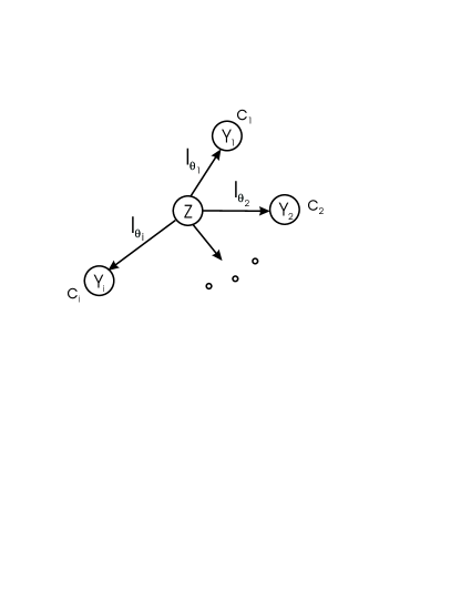
Figure 1: Directed graph of approximation and regularization. Task: estimate unknown source $\mathbf{Z}$ by assuming parameterized $\theta_{i}$ transforms, i.e., certain $l_{\theta_{i}}(\mathbf{Z})$ forms such that the transformed values approximate prescribed values $\mathbf{Y}_{i}$ for all $i=1,2,\ldots$. Estimation means that the quality of approximation as determined by the cumulated costs of each transformation $c_{i}$ is minimum.

In our case, $\mathbf{Z}$ corresponds to state sequences and the parameters of the LRNN system as it will be detailed below.

III.2 LRNN cost function

The following cost function fulfills our requirements

$$f(\Theta,\mathbf{U}) := \lambda_{state}\left\|\cdot\right\|_{state}+\lambda_{appr}\left\|\cdot\right\|_{appr}+\lambda_{\Theta}reg(\Theta)+\lambda_{\mathbf{U}}reg(\mathbf{U})$$

$$(\lambda_{state},\lambda_{appr},\lambda_{\Theta},\lambda_{\mathbf{U}}>0)$$

Here, $reg(\cdot)$ denotes regularization terms, $\Theta$ represents the parameters of the LRNN system ($\Theta:=\left(\mathbf{F},\mathbf{G},\mathbf{H}\right)$), and $\mathbf{U}$ is the internal state sequence ($\mathbf{U}:=\left[\mathbf{u}_{1},\dots,\mathbf{u}_{T}\right]$) and $\mathbf{Z}$ stands for $\Theta$ or $\mathbf{U}$. Optimizations over $\Theta$ and $\mathbf{U}$ were iterated repeatedly. This procedure ensures convergence, at least to a local minimum.

Compact formulation can be gained by introducing matrix $\mathbf{X}$, which represents state sequence and matrices $\mathbf{C}^{b},\mathbf{C}^{e}$, which shall be useful for describing temporal evolutions:

• State sequence matrix $\mathbf{X}:=\left[\mathbf{x}_{1},\dots,\mathbf{x}_{T}\right]$.

• Matrix $\mathbf{C}^{b}$ ((cut-the-beginning) performs transformation

  $$\mathbf{u}_{1},\dots,\mathbf{u}_{T} \rightarrow \mathbf{u}_{2},\dots,\mathbf{u}_{T},$$

  whereas matrix $\mathbf{C}^{e}$ (cut-the-end) acts like

  $$\mathbf{u}_{1},\dots,\mathbf{u}_{T} \rightarrow \mathbf{u}_{1},\dots,\mathbf{u}_{T-1},$$

  $$\mathbf{x}_{1},\dots,\mathbf{x}_{T} \rightarrow \mathbf{x}_{1},\dots,\mathbf{x}_{T-1}.$$

  That is

  $$\mathbf{C}^{b}:=\left[\begin{array}[]{ccccc}0&0&\dots&0\\ 1&0&\dots&0\\ 0&1&0&\dots&\\ \vdots&&\ddots&0\\ 0&\dots&&1\end{array}\right],\mathbf{C}^{e}:=\left[\begin{array}[]{cccc}1&0&\dots&0\\ 0&1&0&\dots\\ \vdots&0&\ddots&0\\ 0&\dots&&1\\ 0&0&\dots&0\end{array}\right]\in\mathbb{R}^{T\times(T-1)}.$$

Now, we can write the approximation property as

$$\left\|\mathbf{H}(\mathbf{FU}+\mathbf{GX})-z\mathbf{X}\right\|\approx 0,$$ (6)

whereas the state equation assumes the following form:

$$\mathbf{UC}^{b}=(\mathbf{FU}+\mathbf{GX})\mathbf{C}^{e}.$$ (7)

Equations (6)-(7) are of affine conditions either in $\mathbf{U}$ or in fixed LRNN parameters $\mathbf{F}$, $\mathbf{G}$, and – in a degenerated sense – also in matrix $\mathbf{H}$. Notice that both (6) and (7) are linear multi-terms in the LRNN parameters and in the internal state, respectively, provided that the other terms are kept constant. Thus, cost function $f$ can be iteratively optimized by alternatively minimizing over $\Theta$ and $\mathbf{U}$. The cost function decreases in every step and, upon convergence, locally optimal parameter set and internal state sequence will be reached, provided that the regularization terms can be managed. Let us consider the $\left\|\mathbf{Z}\right\|_{\mathbf{K}}^{2}$, or $\left\|\mathbf{Z}\right\|_{\mathbf{R}}$ regularization expressions. Such regularization terms

• can be seen as linear multi-terms (of unit length in $\mathbf{Z}$)

• ensure uniqueness in each iterative step if $\mathbf{K}=\mathbf{I}$ and $\epsilon=0$ (i.e., in $L_{1}$ norm).

The latter condition corresponds to sparsification Olshausen and Field (1997); Hoyer (2003).

For the sake of simplicity in the form of the equations, we shall restrict our considerations to $\Theta:=\mathbf{F}$. We shall study costs that emphasize reconstruction with sparsification

$$f_{s}(\mathbf{F},\mathbf{U}) := \lambda_{appr}\left\|\mathbf{H}(\mathbf{FU}+\mathbf{GX})-z\mathbf{X}\right\|_{\mathbf{R}}$$ (8)

$$+\lambda_{state}\left\|(\mathbf{FU}+\mathbf{GX})\mathbf{C}^{e}-\mathbf{UC}^{b}\right\|_{\mathbf{R}}+\lambda_{\mathbf{F}}\left\|\mathbf{F}\right\|_{1}+\lambda_{\mathbf{U}}\left\|\mathbf{U}\right\|_{1}.$$

Cost function $f_{s}$ is made of $\epsilon$-insensitive terms ($\mathbf{R}$ with $\epsilon\geq 0$) of Support Vector Machines (SVMs, see, e.g., Vapnik (1995); Evgeniou et al. (2000); Herbrich (2002) and the references therein). This separation of the $L_{1}$ and $\epsilon$-insensitive norms is somewhat arbitrary. Both norms are used in order to demonstrate the diversity enabled by the mathematical framework. Different combinations are, of course, possible, but no effort was made to find the better combination.

For comparison, we shall study systems equipped with quadratic cost function $f_{q}$:

$$f_{q}(\mathbf{F},\mathbf{U}) := \lambda_{appr}\left\|\mathbf{H}(\mathbf{FU}+\mathbf{GX})-z\mathbf{X}\right\|^{2}$$ (9)

$$+\lambda_{state}\left\|(\mathbf{FU}+\mathbf{GX})\mathbf{C}^{e}-\mathbf{UC}^{b}\right\|^{2}+\lambda_{\mathbf{F}}\left\|\mathbf{F}\right\|^{2}+\lambda_{\mathbf{U}}\left\|\mathbf{U}\right\|^{2}.$$

III.3 Optimization of cost functions

We shall simplify the description by transcribing cost functions $f_{s}$ and $f_{q}$ into vectorial form. As it has been noted before, each term – irrespective of its $\epsilon$-insensitive or quadratic nature – can be seen as a linear multi-term in the corresponding iteration step. Thus, it is sufficient to consider two types of costs:

$$f_{1}(\mathbf{Z}) := \lambda\left\|\sum\limits_{i=1}^{n}\mathbf{L}_{i}\mathbf{Z}\mathbf{M}_{i}-\mathbf{N}\right\|_{\mathbf{R}}\rightarrow\min_{\mathbf{Z}},$$ (10)

$$f_{2}(\mathbf{Z}) := \lambda\left\|\sum\limits_{i=1}^{n}\mathbf{L}_{i}\mathbf{Z}\mathbf{M}_{i}-\mathbf{N}\right\|^{2}_{\mathbf{K}}\rightarrow\min_{\mathbf{Z}},$$ (11)

where $\mathbf{Z}$ denotes the variable subject to optimization in the given step, i.e. $\mathbf{F}$, or $\mathbf{U}$. Such terms can be added to form the full cost functions $f_{s}$ and $f_{q}$, respectively. We shall make use of the forms:

$$vec(\mathbf{BCD}) = (\mathbf{D}^{T}\otimes\mathbf{B})vec(\mathbf{C}),$$ (12)

$$tr(\mathbf{B}^{T}\mathbf{C}) = vec(\mathbf{B})^{T}vec(\mathbf{C}),$$ (13)

$$tr\left(\mathbf{BX}^{T}\mathbf{CYD}\right) = vec(\mathbf{X})^{T}\left[\left(\mathbf{B}\otimes\mathbf{I}_{size(\mathbf{X},1)}\right)^{T}\left(\mathbf{D}^{T}\otimes\mathbf{C}\right)\right]vec(\mathbf{Y}).$$ (14)

For the derivation of Eqs. (12) and (13), see Minka (1997). The derivation of Eq. (14) as well as other details can be found in the Appendix. We have

$$\min_{\mathbf{Z}}f_{1}(\mathbf{Z})\Leftrightarrow$$

$$\Leftrightarrow \min_{\mathbf{y}}\mathbf{w}^{T}\mathbf{y}\text{, provided that }\{\mathbf{Dy}\leq\mathbf{q}\}\text{, where}$$

$$\mathbf{y}:=\left[\begin{array}[]{l}\mathbf{z}\\ \mathbf{a}\\ \mathbf{a}^{*}\end{array}\right],\mathbf{w}:=\left[\begin{array}[]{c}\mathbf{0}\\ \lambda\mathbf{e}\\ \lambda\mathbf{e}\end{array}\right],\mathbf{M}_{\mathbf{L}}:=\sum\limits_{i=1}^{n}\mathbf{M}_{i}^{T}\otimes\mathbf{L}_{i},$$

$$\mathbf{D}:=\left[\begin{array}[]{rrr}\mathbf{M}_{\mathbf{L}}&-\mathbf{I}&\mathbf{0}\\ -\mathbf{M}_{\mathbf{L}}&\mathbf{0}&-\mathbf{I}\\ \mathbf{0}&-\mathbf{I}&\mathbf{0}\\ \mathbf{0}&\mathbf{0}&-\mathbf{I}\end{array}\right],\mathbf{q}:=\left[\begin{array}[]{l}\mathbf{r}+\mathbf{n}\\ \mathbf{r}-\mathbf{n}\\ \mathbf{0}\\ \mathbf{0}\end{array}\right].$$

$$f_{2}(\mathbf{Z}) = \frac{1}{2}\mathbf{z}^{T}\mathbf{H}\mathbf{z}+\mathbf{f}^{T}\mathbf{z}\,(+const)\text{, where }\mathbf{Z}\in\mathbb{R}^{size(\mathbf{Z},1)\times size(\mathbf{Z},2)}.$$

Optimizations can be executed by simply collecting the representative terms, because all terms are either in linear or in quadratic forms.

IV Experimental studies

In the numerical studies, advantages of the joined parameter and representational sparsification – to be referred to as the ‘sparse case’ – were explored for the LRNN architecture. The error of the approximation was monitored as a function of iteration number. The following test examples were chosen:

MG-17,MG-30:

The Mackey-Glass time series were originally introduced for modelling the behavior of blood cells Mackey and Glass (1977) using delayed difference equations:

$$\dot{x}_{t}=\frac{ax_{t-\tau}}{1+x^{c}_{t-\tau}}-bx_{t}.$$

This equation is one of the standard benchmark tests. We used the usual parameterizations of the Mackey-Glass time series ($a=0.2,b=0.1,c=10,\tau=17$ and $30$) under sampling time equal to $6s$. The time series was computed by $4^{th}$ order Runge-Kutta method.

FIR-Laser:

This time series is series ‘$A$’ of the competition at Santa Fe on time series prediction Weigend and Gershenfeld (1993). It is the measured intensity pattern of far infrared (FIR) laser in its chaotic state. The time series will be referred to as FIR-Laser series.

Henon:

The dynamical model

$$x_{t+1} = 1-ax_{t}^{2}+y_{t},$$

$$y_{t+1} = bx_{t}$$

was proposed by Henon Henon (1976). We use standard parameters ($a=1.4$, $b=0.3$), generate the Henon-attractor from pair $(x_{t},x_{t-1})$, and predict $x_{t}$.

We shall approximate one dimensional series ($d_{\mathbf{x}}=1$) of length $T$ with LRNN. 10 different $T$ values ($T=10,20,\ldots 100$) shall be used. Matrix $\mathbf{H}$, which approximates the output from the hidden activites of the LRNN, is a projection to the first coordinate.

Observation, that is matrix $\mathbf{H}$ of the LRNN, shall be the projection to the first coordinate Each coordinates of matrices $\mathbf{F},\mathbf{G}$ were initialized by drawing them independently from the uniform distribution over $[0,1]$. $\epsilon$-insensitivity was chosen as 0.05, that is, $\mathbf{R}=0.05\mathbf{E}$. The dimension of the hidden state was set to $d_{u}=4$.

Normalization steps were applied to allow quantitative comparisons:

• Time series were scaled to vary between $[-1,1]$.

• The $\lambda$’s of Eqs. (8) and (9) were chosen to allow for similar contributions for every term, independently from the dimension of the hidden state of the RNN and the number of the adjustable parameters:

  $$\lambda_{appr}=\frac{1}{Td_{\mathbf{x}}},\quad\lambda_{state}=\frac{1}{(T-1)d_{\mathbf{u}}},\quad\lambda_{\mathbf{U}}=\frac{1}{Td_{\mathbf{u}}},\quad\lambda_{\mathbf{F}}=\frac{1}{d_{\mathbf{u}}^{2}}\text{ .}$$

Optimizations for the sparse case [see Eq. (8)] were compared with optimizations using quadratic cost function [Eq. (9)]. There is a large diversity of possible mixed cost functions. No effort was made to select the main contributing terms to the differences in our results. Such differences might change from problem to problem.

IV.1 Results

Optimization warrant locally optimal solutions. To overcome this problem, in each particular experiment, 20 random initializations of matrices $\mathbf{F}$ and $\mathbf{G}$ were made and 20 different optimizations were executed. Averages of the costs $f_{q}$ and $f_{s}$ were computed and shall be depicted.

Approximation error as a function of iteration number is shown in Fig. 2 for the case of the MG-30 problem. Results are averaged over 20 experiments. Similar results were found in the other experiments, too. Time series of different length were tried. According to the figure, sparsification has its advantages, it makes convergence faster and more uniform:

The approximation produced small errors for the quadratic norm up the lengths about 50. The iteration number required for approximate convergence (the ‘knees’ of the curves) was below 10. For time series having lengths between 50 and 100, the error increased considerably and the typical iteration number required for approximate convergence increased to 20. One may say that up to 100 step long time series and for the quadratic case, 20 iterations are satisfactory to reach stable approximation error, i.e., the close neighborhood of the local minimum.

For the sparse case, the situation is different. Convergence is very fast, 6 iterations were satisfactory to reach stable approximation error in all cases. Errors converged in a few steps.

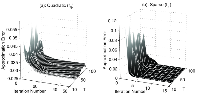
Figure 2: Performance under quadratic cost and for the sparse case. Approximation error versus iteration number and the length of the time series ($T$) approximated for the case of the MG-30 problem. Results are averaged over 20 random experiments. (a): ($f_{q}$); the case for quadratic cost function. (b): ($f_{s}$); the sparse case. Convergence speed of iteration is faster for the sparse case – note the differences in scales.

Predictions of the optimized LRNNs are shown in Fig. 3 for 100 time steps. Sparsification again shows improved interpolating capabilities. This impression is reinforced by Fig. 4, which depicts averages of 20 randomly initialized computations, alike to the one shown in Fig. 3. Averaged prediction errors, that is $\lambda_{appr}\left\|\mathbf{H}(\mathbf{FU}+\mathbf{GX})-z\mathbf{X}\right\|^{2}$ and $\lambda_{appr}\left\|\mathbf{H}(\mathbf{FU}+\mathbf{GX})-z\mathbf{X}\right\|_{\mathbf{R}}$ values for the quadratic and for the sparse case are depicted in the figure. Respective standard deviations as well as the best and the worst cases are also provided.

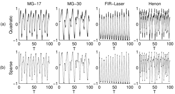
Figure 3: Predictions of LRNN systems trained by different methods and for different problems. Problem set: MG-17, MG-30, FIR-Laser, Henon systems are shown in columns 1, 2, 3, and 4, respectively. (a): ‘Quadratic’, prediction for quadratic cost function. (b): ‘Sparse’, prediction for the sparse case. Length of approximated time series: 100. Black: original time series. Gray: approximation. For detailed results, see, Fig. 4.

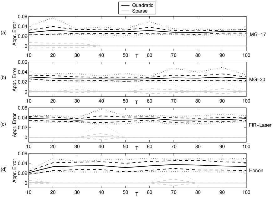
Figure 4: Prediction error averaged over 20 experiments. Experiments are averaged over 20 randomly initialized and optimized LRNN models for the 4 time series examples ((a): MG-17, (b): MG-30, (c): FIR-Laser, (d): Henon). Horizontal axis: time $T$. Vertical axis: error. Solid line: averaged magnitude. Dashed line: standard deviation. Dotted line: best and worst cases. Black: results for quadratic cost function. Gray: results for the sparse case. Prediction error averaged over $T$ is on the order of $10^{-4}$ for the gray curves. See also Table 1.

Table 1 shows small errors for the $\epsilon$-insensitive norm.

Table 1: Time averaged prediction error for the $\epsilon$-insensitive cost.

MG-17	MG-30	FIR-Laser	Henon
$3.3\cdot 10^{-4}$	$4.6\cdot 10^{-4}$	$1.3\cdot 10^{-4}$	$3\cdot 10^{-4}$

According to Fig. 4, the deviation from the average is also small for long intervals, but – due to the nature of this cost function, which measures costs relative to 0.05 – sometimes it is relatively large. The comparison of the different costs is somewhat arbitrary. For time series generated by MG-17, MG-30, FIR-Laser, and Henon systems, the LRNN trained by joined parameter and representational sparsification seems to exhibit a factor of three better approximation than the LRNN using the quadratic norm. Such crude estimation can be gained by comparing 0.158, (the square root of 0.025, which is an approximate low value for the error of the quadratic norm (Fig. 2)) with the value of $\epsilon=0.05$, the estimation for the sparse case from above. We have compared the normalized root mean square error for the two norms: If the measured value is $o_{t}$ and the target is $x_{t}$ then

$$NMRSE:=\frac{\sqrt{\langle(o_{t}-x_{t})^{2}\rangle}}{\sqrt{\langle(x_{t}-\langle x_{t}\rangle)^{2}\rangle}},$$

where $\langle\cdot\rangle$ denotes averaging over $t$. For the quadratic and the $\epsilon$-insensitive cases we received roughly $NRMSE=0.3$ and $NRMSE=0.08$, respectively. That is, comparison using NRMSE, which favors the quadratic norm, there is an advantage of a factor 3 for the $\epsilon$-insensitive norm.

Finally, we note that long term prediction is hard for the linear approach: Apart from a zero measure subset, linear recurrent networks either converge or diverge exponentially.

V Discussions

First, let us mention that convergence of certain sparsification methods can be questioned Olshausen (1996). The method we presented makes use of the $L_{1}$ norm for sparsification, warrants convergence and is an extension of previous architectures, which did not consider a hidden predictive model.

We should address the following questions:

1. What is the advantage of sparse representation?

2. What is the advantage of weight sparsification, or pruning?

Question 1 is intriguing, because neuronal coding seem to apply sparsification as the basic strategy. Neuronal firing in the brain is sparse, which could serve the minimization of energy consumption Baddeley (1996). It is now well established that joint constraints of sparsification and reconstruction (i.e., generative) capabilities produce receptive fields similar to those found in the primary visual cortex Olshausen and Field (1996). More sophisticated architectures, which also apply sparsification can reproduce more details of the receptive fields Rao and Ballard (1999).

Are there other advantages beyond energy minimization? Recently, independent component analysis (ICA) Jutten and Herault (1991); Comon (1994); Bell and Sejnowski (1995), an information transfer optimizing scheme, has been related to sparsification Hyvärinen (1999). It has been shown that ICA and appropriate thresholding corresponds to well established denoising methods. Denoising, that is the removal of structureless high entropy portion of the input and the uncovering of structures are important tasks for learning. Subliminal statistical learning is indeed, a strategy applied by the brain Watanabe et al. (2001). ICA with denoising capabilities, called sparse code shrinkage (SCS) Hyvärinen (1999), enables local noise estimation and local noise filtering. SCS is most desirable, because it optimizes noise filtering with respect to the experienced inputs.

Another advantage emerges if sparsified representation is embedded into reconstruction networks. This construct can produce overcomplete representations Olshausen and Field (1996) which, by construction, exhibit graceful degradation. Also, overcomplete representations can produce very different outputs for similar inputs, a most desirable feature for categorization and decision making.

It is easy to see that norm $L_{1}$ biases the system towards sparse representation compared to the $L_{2}$ norm: The $L_{1}$ norm produces larger costs for small signals and depresses small signals more efficiently. This statement seems more general, because the $\epsilon$-insensitive cost function is closely related to sparsification networks Girosi (1998).

There are different noise models behind the $L_{1}$ and the $L_{2}$ norms. In such considerations, the norm of the approximation is seen as the log-likelihood of the distribution of the noise. The $L_{1}$ and the $L_{2}$ norms, as well as that of the $epsilon$-insensitive norm are all incorporated into the following log-likelihood expression Pontil et al. (2000):

$$V(x)=-\log\int_{0}^{\infty}d\beta\int_{-\infty}^{\infty}dt\sqrt{\beta}e^{-\beta(x-t)^{2}}P(\beta,t),$$ (17)

where $x$ is the argument of the respective norms. For example, quadratic loss function emerges if $P(\beta,t)=\delta(\beta-\frac{1}{2\sigma^{2}})\delta(t)$, where $\delta(.)$ is Dirac’s delta function. The $L_{1}$ loss is recovered by setting $P(\beta,t)=\beta^{2}\exp(-\frac{1}{4\beta^{2}})\delta(t)$. The expression for $\epsilon$-insensitive loss in a factorized form for $P(\beta,t)$ is as follows: $P(\beta,t)=\frac{C}{\beta^{2}}\exp(-\frac{1}{4\beta^{2}})\lambda_{\epsilon}(t)$, where $\lambda_{\epsilon}(t)=\frac{1}{2(\epsilon+1)}\left(\chi_{[-\epsilon,\epsilon]}(t)+\delta(t-\epsilon)+\delta(t+\epsilon)\right)$, $\chi_{[-\epsilon,\epsilon]}$ is the characteristic function of the interval $[-\epsilon,\epsilon]$, and C is a normalization constant. The interpretation is that the noise affecting the data is additive and Gaussian, but its mean can be different from zero. The variance and mean of the noise are random variables with given probability distributions. For diminishing range of the non-zero mean Gaussian distributions, the expression approximates the $L_{1}$ norm Pontil et al. (2000). In turn, both the $L_{1}$ norm and the $\epsilon$-insensitive norm correspond to super-Gaussian noise distributions.

Concerning Question 2, sparsification of weight matrices, e.g., exponential forgetting, pruning of weights, as well as other computational means have been studied over the years. The interested reader is referred to the literature on this broad field Haykin (1999). Question 2 seems to have a particular advantage, called the Occam’s razor principle. In reverse engineering, such as the search for the (hidden) parameters of an LRNN, there are many solutions having identical or similar properties. All of these could be the the solution of the task. Which one is the right one? Or, at least, which one is the most probable? The answer of the philosopher is that the simplest explanation, that is, the one that makes the least assumptions is the best, or the most probable. Similar ideas have emerged in information theory, within the context of Kolmogorov complexity Cover and Thomas (1991). A bridge has been built to connect the idea of least number of assumptions and concepts of complexity. This is the minimum description length principle Rissanen (1978), which makes use of complexity measures both for the data and for the assumed family of probability distributions, that is for the model. The best, i.e., the most probable description, has the minimum complexity. Important connections between the minimum description length principle and regularization theory have been worked out in the literature MacKay (1992); Hinton and Zemel (1994). For a recent review on this subject, see Chen and Haykin (2002). One may think of weight sparsification as a method, which decreases the number of parameters and thus searches for simpler descriptions, provided that the precision of the parameters is bounded.

Our results indicate that local minima are better distributed for $L1$ and/or $\epsilon$-insensitive norms than for the $L_{2}$ norm within the problem set we studied. However, it is known that there should be other problem sets, where the quadratic cost is superior to the absolute value Wolpert and MacReady (1997). It is easy to create an example: quadratic cost on the parameters suits parameter sets, which exhibit Gaussian distribution. In turn, the success of the $L_{1}$ and $\epsilon$-insensitive norms raises the question about the type of problems, which profit from this cost function family.

We need to examine the statistical properties of phenomena in nature. It seems that these phenomena have special distributions. The distributions are super-Gaussian, sometimes exponential and sometimes they have very heavy tails, e.g., they can be characterized by power-law distribution in a broad range. This looks typical for natural forms (c.f. fractals) and evolving/developing systems (see, e.g., Albert and Barab si (2002) and references therein).

We have measured the four time series: Mackey-Glasses (MG-17, MG-30), FIR-Laser, Henon. The distribution of distances between zero crossings of time series of 10,000 step long were analyzed.

1. The kurtosis of the experienced distributions were computed, according to

   $$kurtosis(X)=\frac{E\left[X-\mu\right]^{4}}{\sigma^{4}}-3,$$

   where $E$ denotes expectation value, $\mu$ is the mean of variable $X$, $\sigma$ is its standard deviation. Positive kurtosis is typical for super-Gaussian distributions, which have heavy tails. Results are shown in Table 2.

   Table 2: Kurtosis of distances between zero-crossings

   MG-17	MG-30	FIR-Laser	Henon
   -0.92	1.11	101.8	2.89

   For all cases, but the MG-17 series, positive kurtosis was found. It is known, however, that series MG-17 is at the borderline of chaos: the Mackey-Glass time series becomes chaotic if $\tau>16.8$.

2. The second study concerned the power law behavior. It was found that the zero crossings for the Henon and the MG-30 systems approximate power-law distributions, the MG-17 series does not, and the FIR laser is in between: it exhibits an erratic descending curve on log-log scale. The slope of the log-log fits were smaller smaller than $-1$, except for the MG-17 time series.

The problems we studied, typically have heavy tailed distributions. In turn, the $L_{1}$ and/or the $\epsilon$-insensitive norms suit such problems better than $L_{2}$ norm, because the $L_{1}$ norm corresponds to the Laplace (i.e., double sided exponential) distribution, which has a heavier tail than the Gaussian distribution. Power-law distributions, however, are even more at the extremes in this respect. Because such heavy tailed distributions are typical in nature (see, e.g., Bak (1996); Holland (1998)), one may find even better norms when identification of emergent behaviors is the issue.

VI Conclusion

We have put forth a joint formalism for sparsification of both the representation and the structure of neural networks. The approximation was applied to a recurrent neural network and the joined effect was studied. Experiments were conducted on a number of benchmark problems, such as the Mackey-Glass with parameters 17–30, the emission of a far-infrared laser, and the Henon time series. Our results suggest that the joined constraint on sparsification is advantageous on these examples. Namely, optimizations were faster and had local optima exhibited better interpolating properties for the sparsified case than for traditional quadratic norm. We have argued that these findings are due to the underlying statistics of these phenomena: quadratic norms assume Gaussian noise and distributions with heavy-tails are be better approximated by norms with lower degrees. Joint advantages of the removal of structureless high entropy, a feature of representational sparsification, and the discovery of structures with sparse networks needs to be further explored.

Appendix A Derivation of Eq. (14)

$$tr\left(\mathbf{BX}^{T}\mathbf{CYD}\right) = tr\left[\left(\mathbf{XB}^{T}\right)^{T}\left(\mathbf{CYD}\right)\right]$$

$$= vec\left(\mathbf{IXB}^{T}\right)^{T}vec\left(\mathbf{CYD}\right)$$

$$= \left[\left(\mathbf{B}\otimes\mathbf{I}\right)vec\left(\mathbf{X}\right)\right]^{T}\left[\left(\mathbf{D}^{T}\otimes\mathbf{C}\right)vec(\mathbf{Y})\right]$$

$$= vec(\mathbf{X})^{T}\left[\left(\mathbf{B}\otimes\mathbf{I}_{size(\mathbf{X},1)}\right)^{T}\left(\mathbf{D}^{T}\otimes\mathbf{C}\right)\right]vec(\mathbf{Y}).$$

Appendix B Computing the norms

$$\min_{\mathbf{Z}}f_{1}(\mathbf{Z})\Leftrightarrow$$

$$\Leftrightarrow \min_{\{\mathbf{Z},\mathbf{A}^{(*)}\}}\left\{\lambda tr\left[\mathbf{E}^{T}\left(\mathbf{A}+\mathbf{A}^{*}\right)\right]\right\},$$

$$\text{provided that }\left\{\begin{array}[]{rll}\sum\limits_{i=1}^{n}\mathbf{L}_{i}\mathbf{Z}\mathbf{M}_{i}-\mathbf{N}&\leq&\mathbf{R}+\mathbf{A}\\ -\left(\sum\limits_{i=1}^{n}\mathbf{L}_{i}\mathbf{Z}\mathbf{M}_{i}-\mathbf{N}\right)&\leq&\mathbf{R}+\mathbf{A}^{*}\\ \mathbf{0}&\leq&\mathbf{A}^{(*)}\\ \end{array}\right\}.$$

$$\Leftrightarrow \min_{\{\mathbf{Z},\mathbf{A}^{(*)}\}}\left[\lambda vec(\mathbf{E})^{T}(vec(\mathbf{A})+vec(\mathbf{A}^{*})\right]=:\left[\lambda\mathbf{e}^{T}(\mathbf{a}+\mathbf{a}^{*})\right],$$

$$\text{provided that }\left\{\begin{array}[]{rlll}\sum\limits_{i=1}^{n}\left(\mathbf{M}_{i}^{T}\otimes\mathbf{L}_{i}\right)\mathbf{z}&-\mathbf{a}&\leq&\mathbf{r}+\mathbf{n}\\ -\sum\limits_{i=1}^{n}\left(\mathbf{M}_{i}^{T}\otimes\mathbf{L}_{i}\right)\mathbf{z}&-\mathbf{a}^{*}&\leq&\mathbf{r}-\mathbf{n}\\ &\mathbf{0}&\leq&\mathbf{a}^{(*)}\\ \end{array}\right\}.$$

$$\Leftrightarrow \min_{\mathbf{y}}\mathbf{w}^{T}\mathbf{y}\text{, provided that }\{\mathbf{Dy}\leq\mathbf{q}\}\text{, where}$$

$$\mathbf{y}:=\left[\begin{array}[]{l}\mathbf{z}\\ \mathbf{a}\\ \mathbf{a}^{*}\end{array}\right],\mathbf{w}:=\left[\begin{array}[]{c}\mathbf{0}\\ \lambda\mathbf{e}\\ \lambda\mathbf{e}\end{array}\right],\mathbf{M}_{\mathbf{L}}:=\sum\limits_{i=1}^{n}\mathbf{M}_{i}^{T}\otimes\mathbf{L}_{i},$$

$$\mathbf{D}:=\left[\begin{array}[]{rrr}\mathbf{M}_{\mathbf{L}}&-\mathbf{I}&\mathbf{0}\\ -\mathbf{M}_{\mathbf{L}}&\mathbf{0}&-\mathbf{I}\\ \mathbf{0}&-\mathbf{I}&\mathbf{0}\\ \mathbf{0}&\mathbf{0}&-\mathbf{I}\end{array}\right],\mathbf{q}:=\left[\begin{array}[]{l}\mathbf{r}+\mathbf{n}\\ \mathbf{r}-\mathbf{n}\\ \mathbf{0}\\ \mathbf{0}\end{array}\right].$$

$$f_{2}(\mathbf{Z}) = \lambda tr\left[\left(\sum\limits_{i=1}^{n}\mathbf{L}_{i}\mathbf{Z}\mathbf{M}_{i}-\mathbf{N}\right)^{T}\mathbf{K}\left(\sum\limits_{j=1}^{n}\mathbf{L}_{j}\mathbf{Z}\mathbf{M}_{j}-\mathbf{N}\right)\right]$$

$$= \lambda tr\left[\sum\limits_{i,j}\mathbf{M}_{i}^{T}\mathbf{Z}^{T}\left(\mathbf{L}_{i}^{T}\mathbf{K}\mathbf{L}_{j}\right)\mathbf{Z}\mathbf{M}_{j}-2\sum\limits_{j}\mathbf{N}^{T}\mathbf{K}\mathbf{L}_{j}\mathbf{Z}\mathbf{M}_{j}+\mathbf{N}^{T}\mathbf{K}\mathbf{N}\right]$$

$$= \frac{1}{2}vec(\mathbf{Z})^{T}\left(2\lambda\sum\limits_{i,j}\left\{\left(\mathbf{M}_{i}^{T}\otimes\mathbf{I}_{size\left(\mathbf{Z},1\right)}\right)^{T}\left[\mathbf{M}_{j}^{T}\otimes\left(\mathbf{L}_{i}^{T}\mathbf{K}\mathbf{L}_{j}\right)\right]\right\}\right)vec(\mathbf{Z})$$

$$+\left[-2\lambda\sum\limits_{j}vec(\mathbf{L}_{j}^{T}\mathbf{K}\mathbf{N}\mathbf{M}_{j}^{T})\right]^{T}vec(\mathbf{Z})+\lambda tr\left(\mathbf{N}^{T}\mathbf{K}\mathbf{N}\right)$$

$$=: \frac{1}{2}\mathbf{z}^{T}\mathbf{H}\mathbf{z}+\mathbf{f}^{T}\mathbf{z}\,(+const)\text{, where }\mathbf{Z}\in\mathbb{R}^{size(\mathbf{Z},1)\times size(\mathbf{Z},2)}.$$

Optimizations can be executed by simply collecting the representative terms, because all terms are either in linear or in quadratic forms.

References

- Bak (1996) P. Bak, How Nature works: The science of self-organized criticality (Copernicus, New York, 1996).
- Holland (1998) J. Holland, Emergence: From Order to Chaos (Perseus Books, Cambridge, Ma., 1998).
- Jensen (1998) H. Jensen, Self-organized criticality (Cambridge University Press, Cambridge, UK, 1998).
- Johnson (2001) S. Johnson, Emergence: The Connected Lives of Ants, Brains, Cities, and Software (Scribner, New York, 2001).
- Albert and Barab si (2002) R. Albert and A. Barab si, Reviews of Modern Physics 74, 47 (2002).
- Lodding (2004) K. Lodding, QUEUE pp. 66–76 (2004).
- Korn and Faure (2003) H. Korn and P. Faure, Comptes Rendus Biologies 326, 787 (2003).
- Gauthier (2003) D. Gauthier, Am. J. Phys. 71, 750 (2003).
- Sanger (1989) D. Sanger, Connection Science 1, 115 (1989).
- Levin et al. (1994) A. Levin, T. Leen, and J. Moody, in Advances in Neural Information Processing Systems, edited by J. D. Cowan, G. Tesauro, and J. Alspector (Morgan Kaufmann, San Mateo, CA, 1994), vol. 6, pp. 35–42.
- Deco et al. (1995) G. Deco, W. Finnoff, and H. Zimmermann, Neural Computation 7, 86 (1995).
- Reed et al. (1995) R. Reed, R. Marks, and S. Oh, IEEE Transactions on Neural Networks 6, 529 (1995).
- Kamimura (1997) R. Kamimura, Neural Computation 9, 1357 (1997).
- Olshausen and Field (1997) B. Olshausen and D. Field, Sparse coding with an overcomplete basis set: A strategy employed by v1? (1997), URL citeseer.ist.psu.edu/olshausen96sparse.html.
- Olshausen and Field (1996) B. Olshausen and D. Field, Nature pp. 607–609 (1996).
- Koene and Takane (1999) R. Koene and Y. Takane, Neural Computation 11, 783 (1999).
- Chen and Haykin (2002) Z. Chen and S. Haykin, Neural Computation 14, 2791 (2002).
- Olshausen and Field (2004) B. Olshausen and D. Field, Current Opinion in Neurobiology 14, 1 (2004).
- Hinton (1989) G. Hinton, Artificial Intelligence 40, 185 (1989).
- Williams (1994) P. Williams, Neural Computation 7, 117 (1994).
- Hyvärinen and Karthikesh (2000) A. Hyvärinen and R. Karthikesh, in Proc. Int. Workshop on Independent Component Analysis and Blind Signal Separation (ICA2000) (Helsinki, Finland, 2000), pp. 477–452.
- Szatmáry et al. (2002) B. Szatmáry, B. Póczos, J. Eggert, E. Körner, and A. Lőrincz, in Proc. of the 15th European Conference on Artificial Intelligence, edited by F. van Harmelen (IOS Press, Amsterdam, NL, 2002), ECAI 2002, pp. 503–507.
- Haykin (1999) S. Haykin, Neural networks: A comprehensive foundation (Prentice-Hall, Upper Saddle River, NJ, 1999), 2nd ed.
- Vapnik (1998) V. Vapnik, Statistical Learning Theory (Wiley, Chichester, GB, 1998).
- Evgeniou et al. (2000) T. Evgeniou, M. Pontil, and T. Poggio, Advances in Computational Mathematics 13, 1 (2000).
- Tsoi and Back (1997) A. Tsoi and A. Back, Neurocomputing 15, 183 (1997).
- Vapnik (1995) V. Vapnik, The nature of statistical learning theory (Springer-Verlag New York, Inc., 1995), ISBN 0-387-94559-8.
- Hoyer (2003) P. Hoyer, Neurocomputing (2003).
- Herbrich (2002) R. Herbrich, Learning Kernel Classifiers (The MIT Press, 2002).
- Minka (1997) T. Minka, Old and new matrix algebra useful for statistics, Available at citeseer.ist.psu.edu/minka97old.html (1997).
- Mackey and Glass (1977) M. Mackey and L. Glass, Science pp. 287–289 (1977).
- Weigend and Gershenfeld (1993) A. Weigend and N. Gershenfeld, Time Series Prediction: Forecasting the Future and Understanding the Past (Addison Wesley, 1993).
- Henon (1976) M. Henon, Communications in Mathematical Physics (1976).
- Olshausen (1996) B. A. Olshausen, A.I. Memo 1580, MIT AI Lab (1996), c.B.C.L. Paper No. 138.
- Baddeley (1996) R. Baddeley, Nature 381, 560 (1996).
- Rao and Ballard (1999) R. Rao and D. Ballard, Nature Neuroscience 2, 79 (1999).
- Jutten and Herault (1991) C. Jutten and J. Herault, Signal Processing 24, 1 (1991).
- Comon (1994) P. Comon, Signal Processing 36, 287 (1994).
- Bell and Sejnowski (1995) A. Bell and T. Sejnowski, Neural Computation 7, 1129 (1995).
- Hyvärinen (1999) A. Hyvärinen, Neural Computation 11, 1739 (1999).
- Watanabe et al. (2001) T. Watanabe, J. Nanez, and Y. Sasaki, Nature 413, 844 (2001).
- Girosi (1998) F. Girosi, Neural Computation 10, 1455 (1998).
- Pontil et al. (2000) M. Pontil, S. Mukherjee, and F. Girosi, in Proceedings of Algorithmic Learning Theory (Sydney, Australia, 2000), a.I. Memo 1651, MIT Artificial Intelligence Laboratory, Cambridge, MA, 1998.
- Cover and Thomas (1991) T. Cover and J. Thomas, Elements of Information Theory (John Wiley and Sons, New York, USA, 1991).
- Rissanen (1978) J. Rissanen, Automation 14, 465 (1978).
- MacKay (1992) D. MacKay, PhD Thesis, Caltech, USA, Department of Computation and Neural Systems (1992).
- Hinton and Zemel (1994) G. Hinton and R. Zemel, in Advances in Neural Information Processing Systems (Morgan Kaufmann Publishers, 1994), vol. 6, pp. 3–10.
- Wolpert and MacReady (1997) D. Wolpert and W. MacReady, IEEE Trans. on Evolutionary Computing 1, 67 (1997).