Distance properties of expander codes

Abstract.

We study the minimum distance of codes defined on bipartite graphs. Weight spectrum and the minimum distance of a random ensemble of such codes are computed. It is shown that if the vertex codes have minimum distance $\geq 3$, the overall code is asymptotically good, and sometimes meets the Gilbert-Varshamov bound.

Constructive families of expander codes are presented whose minimum distance asymptotically exceeds the product bound for all code rates between 0 and 1.

1. Introduction

1.1. Context

The general idea of constructing codes on graphs first appeared in Tanner’s classical work [19]. One of the methods put forward in this paper was to associate message bits with the edges of a graph and use a short linear code as a local constraint on the neighboring edges of each vertex. M. Sipser and D. Spielman [16] generated renewed interest in this idea by tying spectral properties of the graph to decoding analysis of the associated code: they suggested the term expander codes for code families whose analysis relies on graph expansion. Further studies of expander codes include [23, 11, 5, 4, 3, 17].

While [19] and [16] did not especially favor the choice of an underlying bipartite graph, subsequent papers, starting with [23], made heavy use of this additional feature. In retrospect, codes on bipartite graphs can be viewed as a natural generalization of R. Gallager’s low-density parity-check codes. Another view of bipartite-graph codes involves the so-called parallel concatenation of codes which refers to the fact that message bits enter two or more unrelated sets of parity-check equations that correspond to the local constraints. This view ties bipartite-graph codes to turbo codes and related code families; the bipartite graph can be defined by a permutation of message symbols which is very close to the “interleaver” of the turbo coding schemes.

A more traditional method of code concatenation, dating back to the classical works of P. Elias and G. D. Forney, suggests to encode the message by several codes successively, earning this class of constructions the name serial concatenation. A well-known set of results on constructions, parameters and decoding performance of serial concatenations includes Forney’s bound on the error exponent attainable under a polynomial-time decoding algorithm [9], implying in particular the existence of a constructive capacity-achieving code family, and the Zyablov bound on the relative distance attainable under the condition of polynomial-time constructibility [24]. Initial results of this type for expander codes [16, 23, 5] were substantially weaker than both the Forney and Zyablov bounds, but additional ideas employed both in code construction and decoding led to establishing these results for the class of expander codes [3, 11, 17]. In particular, paper [3] focussed on similarities and differences between serial concatenations and bipartite-graph codes viewed as parallel concatenations. We refer to this paper for a detailed introduction to properties of both code families. Paper [3] also suggested a decoding algorithm that corrects a fraction of errors approaching half the designed distance, i.e. half the Zyablov bound. The error exponent of this algorithm reaches the Forney bound for serial concatenations. The advantage of bipartite-graph codes over the latter is that for them, the decoding complexity is an order of magnitude lower (proportional to the block length $N$ as opposed to $N^{2}$ for serial concatenations).

The main goal of [3] was to catch up with the classical achievements of serial concatenation and show that they can be reproduced by parallel schemes, with the added value of lower-complexity decoding. One of the motivations for the present paper is to exhibit new achievements of parallel concatenation, unrelated to decoding, that surpass the present-day performance of all codes constructed in the framework of the classical serial approach.

1.2. Bounding the minimum distance of expander codes

The main focus of this paper are the parameters $[N,RN,\delta N]$ of bipartite-graph codes, particularly the asymptotic behavior of the relative minimum distance $\delta$ as a function of the rate $R$. Bipartite-graph codes, and more generally codes defined on graphs, are famous for their low-complexity decoding and its performance under high noise, but are generally considered to have poorer minimum distances than their algebraic counterparts. We strive here to reverse this trend and show that it is possible to design codes defined on graphs with very respectable $R$ versus $\delta$ tradeoffs.

In the first half of this paper we study the average weight distribution of the random ensemble of bipartite-graph codes (Section 3). Under the assumption that the minimum distance of the small constituent codes is at least $3$, we show that the ensemble contains codes which are asymptotically good for all code rates, and for some values of the rate reach the Gilbert-Varshamov (GV) bound. This result shows interesting parallels with a similar theorem for serial concatenations in Forney’s sense [7, 21]. It also generalizes the result of [8, 13] where bipartite-graph codes with component Hamming codes were shown to be asymptotically good.

In the second part of the paper we turn to constructive issues. Until now the product of the relative distances of the constituent codes was the standard lower bound on the relative minimum distance of expander codes, as it is for the class of Forney’s serially concatenated codes, including product codes. Efforts have been made to surpass this product bound, or designed distance, for short block lengths, see e.g. [20], but no asymptotic improvements have been obtained for any of these classes. In Section 4 we describe two families of bipartite-graph codes that asymptotically surpasses the product bound on the minimum distance. In particular we obtain a polynomially constructible family of binary codes that for any rate between 0 and 1 have relative distance greater than the Zyablov bound [24]. These constructions are based on allowing both binary and nonbinary local codes in the expander code construction and matching the restrictions imposed by them on the binary weight of the edges in the graph. This result confirms the intuition, supported by examples of short codes and ensemble-average results, of the product bound being a poor estimate of the true distance of two-level code constructions be they parallel or serial concatenations. Even though it does not match the distance of such code families as multilevel concatenations or serial concatenations with algebraic-geometry outer codes, this result is still the first of its kind because all the other constructions rely on the product bound for estimating the designed distance. In particular, the results of Section 4 improve over the parameters of all previously known polynomial-time constructions of expander codes and of concatenations of two codes not involving algebraic-geometry codes, including the constructions of Forney [9, 24], Alon et al. [1], Sipser and Spielman [16], Guruswami and Indyk [11], the authors [5], and Bilu and Hoory [6]. In the final Section 5 we compare construction complexity with other code families whose parameters are comparable to those of the bipartite-graph codes constructed in this paper.

2. Preliminaries

2.1. Bipartite-graph codes: Basic construction

Let $G=(V,E)$ be a balanced, $\Delta$-regular bipartite graph with the vertex set $V=V_{0}\cup V_{1},|V_{0}|=|V_{1}|=n.$ The number of edges is $|E|=N=\Delta n$.

Let us choose an arbitrary ordering of edges of the graph which will be fixed throughout the construction. For a given vertex $v\in G$ this defines an ordering of edges $v(1),v(2),\dots,v(\Delta)$ incident to it. We denote this subset of edges by $E(v)$. For a vertex $v$ in one part of $G$ the set of vertices in the other part adjacent to $v$ will be also called the neighborhood of the vertex $v$, denoted ${\mathcal{N}}(v)$.

Let $A[\Delta,R_{0}\Delta],B[\Delta,R_{1}\Delta]$ be binary linear codes. The binary bipartite-graph code $C(G;A,B)$ has parameters $[N,RN]$. We assume that the coordinates of $C$ are in one-to-one correspondence with the edges of $G$. Let ${\mathbf{x}}\in\{0,1\}^{N}$. By ${\mathbf{x}}_{v}$ we denote the projection of ${\mathbf{x}}$ on the edges incident to $v.$ By definition, ${\mathbf{x}}$ is a codevector of $C$ if

1. for every $v\in V_{0}$, the vector ${\mathbf{x}}_{v}$ is a codeword of $A$;

2. for every $w\in V_{1}$, the vector ${\mathbf{x}}_{w}$ is a codeword of $B$.

This construction and its generalizations are primarily studied in the asymptotic context when $n\to\infty,\Delta=\text{const}.$ Paper [16] shows that, for a suitable choice of the code $A$, codes $C(G;A,A)$ are asymptotically good and correct a fraction of errors that grows linearly with $n$ under a linear-time decoding algorithm. Another decoding algorithm, which gives a better estimate of the number of correctable errors, was suggested in [23]. Paper [5] shows that introducing two different codes $A$ and $B$ enables one to prove that the codes $C(G;A,B)$ attain capacity of the binary symmetric channel. Note that taking $A$ the parity-check code and $B$ the repetition code we obtain Gallager’s LDPC codes. For this reason codes $C(G;A,B)$ are sometimes called generalized low-density codes [8, 13].

Before turning to parameters of the code $C$ let us recall some properties of the graph $G$. Let $\lambda$ be the second largest eigenvalue (of the adjacency matrix) of $G$. For a vertex $v\in V_{0}$ and a subset $T\subset V_{1}$ let $\deg_{T}(v)$ be the number of edges that connect $v$ to vertices in $T$. A key tool for the analysis of the code $C$ is given by the following lemma.

Lemma 1.

[3] Let $S\subset V_{0},T\subset V_{1}.$ Suppose that

$$\forall_{v\in S}\deg_{T}(v)\geq\alpha_{0}\Delta,\quad\forall_{w\in T}\deg_{S}(w)\geq\alpha_{1}\Delta,$$

where $\alpha_{0},\alpha_{1}\in(0,1).$ Then

$$|S|\geq\alpha_{1}n\Big{(}1-\frac{\lambda}{\Delta\alpha_{0}}\Big{)}\Big{(}1-\frac{\lambda}{2\Delta\alpha_{1}}\Big{)}.$$

From this, the relative distance of $C$ satisfies

(1) $$\delta\geq\delta_{0}\delta_{1}\Big{(}1-\frac{\lambda}{d_{0}}\Big{)}\Big{(}1-\frac{\lambda}{2d_{1}}\Big{)},$$

where $d_{0}=\Delta\delta_{0},d_{1}=\Delta\delta_{1}$ are the distances of the codes $A$ and $B$.

The rate of the code $C$ is easily estimated to be

(2) $$R\geq R_{0}+R_{1}-1.$$

We will assume that the second eigenvalue $\lambda$ of the graph $G_{1}=(V_{0}\cup V_{1},E_{1})$ is small compared to its degree $\Delta_{1}$. For instance, the graph $G_{1}$ can be chosen to be Ramanujan, i.e., $\lambda\leq 2\sqrt{\Delta_{1}-1}$. Then from 1 we see that the code $C$ approaches the product bound $\delta_{0}\delta_{1}$ which is a standard result for serial concatenations.

2.2. Multiple edges

In [5] this construction was generalized by allowing every edge to carry $t$ bits of the codeword instead of just one bit, where $t$ is some constant. The code length then becomes $n\Delta t$. We again denote this quantity by $N$ because it will always be clear from the context which of the two constructions we consider. Let $A[t\Delta,R_{0}t\Delta]$ be a binary linear code and $B[\Delta,R_{1}\Delta]$ be a $q$-ary additive code, $q=2^{t}$. To define the code $C(G;A,B)$ we keep Condition 1. above and replace condition 2 with

$2^{\prime}.$ for every $w\in V_{1}$ the vector ${\mathbf{x}}_{w}$, viewed as a $q$-ary vector, is a codeword in $B$.

An alternative view of this construction is allowing $t$ parallel edges to replace each edge in the original graph $G$. Then every edge again corresponds to one bit of the codeword. An advantage of the view offered above is that it allows a direct application of Lemma 1.

In [5] it was shown that this improves the parameters and performance estimates of the code $C$. For instance, there exists an easily constructible code family $C(G;A,A)$ of rate $R$ with relative distance given by

(3) $$\delta\geq\frac{1}{2}(1-R)h^{-1}\Big{(}\frac{1-R}{2}\Big{)}-\varepsilon\qquad(\varepsilon>0)$$

where $h(\cdot)$ is the binary entropy function. Note that the distance estimate is immediate from Lemma 1.

The generalized codes of this section together with some other modifications of the original construction will be used in Sect. 4 below.

Figure 1. Constructions of bipartite-graph codes with multiple edges: (a) Basic construction, (b) Modified construction.

2.3. Modified code construction

Let $G=(V,E)$ be a bipartite graph whose parts are $V_{0}$ (the left vertices) and $V_{1}\cup V_{2}$ (the right vertices), where $|V_{i}|=n$ for $i=0,1,2.$ The degree of the left vertices is $\Delta$, the degree of the vertices in $V_{1}$ is $\Delta_{1}$ and the degree of vertices in $V_{2}$ is $\Delta_{2}=\Delta-\Delta_{1}.$ For a given vertex $v\in V_{0}$ we denote by $E(v)$ the set of all edges incident to it and by $E_{i}(v)\subset E(v),i=1,2$ the subset of edges of the form $(v,w)$, where $w\in V_{i}$. The ordering of the edges on $v$ defines an ordering on $E_{i}(v).$ Note that both subgraphs $G_{i}=(V_{0}\cup V_{i},E_{i}),i=1,2$ can be chosen to be regular, of degrees $\Delta_{1}$ and $\Delta_{2}$ respectively.

Let $A$ be a $[t\Delta,R_{0}t\Delta,d_{0}=t\Delta\delta_{0}]$ linear binary code of rate $R_{0}=\Delta_{1}/\Delta$. The code $A$ can also be seen as a $q$-ary additive $[\Delta,R_{0}\Delta]$ code, $q=2^{t}$. Let $B$ be a $q$-ary $[\Delta_{1},R_{1}\Delta_{1},d_{1}=\Delta_{1}\delta_{1}]$ additive code. We will also need an auxiliary $q$-ary code $A_{\text{aux}}$ of length $\Delta_{1}$. Every edge of the graph will be associated with $t$ bits of the codeword of the code $C$ of length $N=nt\Delta.$ The code $C$ is defined as the set of vectors ${\mathbf{x}}=\{x_{1},\dots,x_{N}\}$ such that

1. For every vertex $v\in V_{0}$ the subvector $(x_{j})_{j\in E(v)}$ is a ($q$-ary) codeword of $A$ and the set of coordinates $E_{1}(v)$ is an information set for the code $A$.

2. For every vertex $v\in V_{1}$ the subvector $(x_{j})_{j\in E(v)}$ is a codeword of $B$;

3. For every vertex $v\in V_{0}$ the subvector $(x_{j})_{j\in E_{1}(v)}$ is a codeword of $A_{\text{aux}}.$

Both this construction and the construction from the previous subsection are illustrated in Fig. 1.

We will choose the minimum distance $d_{\text{aux}}=\delta_{\text{aux}}\Delta_{1}$ of the code $A_{\text{aux}}$ so as to make the quantity $\lambda/d_{\text{aux}}$ arbitrarily small, where $\lambda$ is the second eigenvalue of $G_{1}$. By choosing $\Delta_{1}$ large enough, the rate $R_{\text{aux}}$ of $A_{\text{aux}}$ can be thought of as a quantity such that $1-R_{\text{aux}}$ is almost $\mathcal{O}(1/\sqrt{\Delta}).$

This construction was introduced and studied in [4, 3]. The code $C$ has the parameters $[N=nt\Delta,RN,D].$ The rate $R$ is estimated easily from the construction:

(4) $$R\geq R_{0}R_{1}-R_{0}(1-R_{\rm aux}),$$

which can be made arbitrarily close to $R_{0}R_{1}$ by choosing $\Delta$ large enough but finite.

The distance $D$ of the code $C$ can be again estimated from Lemma 1 applied to the subgraph $G_{1}.$ Then we have $\alpha_{0}=\delta_{\rm aux},\alpha_{1}=\delta_{1},$ and

(5) $$D\geq\delta_{0}\delta_{1}\left(1-\frac{\lambda}{d_{\rm aux}}\right)\left(1-\frac{\lambda}{2d_{1}}\right)N.$$

This means in particular that the relative minimum distance $D/N$ is bigger than a quantity that can be made arbitrarily close to the product $\delta_{0}\delta_{1}$. Together with (4) this means that the distance of the code $C$ for $n\to\infty$ can be made arbitrarily close to the product, or Zyablov bound [24]

(6) $$\delta_{\text{Z}}(R)=\max_{R\leq x\leq 1}\delta_{\text{\rm GV}}(x)(1-R/x).$$

This result was proved in [3].

Alternative description of the modified construction. The above code can be thought of as a serially concatenated code with $A$ as inner binary code and a $Q$-ary outer code with $Q=2^{t\Delta_{1}}.$ The outer code is formed by viewing the binary $t\Delta_{1}$-tuple indexed by the edges of $G_{1}$ incident to a vertex of $V_{0}$ as an element of the $Q$-ary alphabet. The $Q$-ary cod $B^{\prime}$ is defined by conditions 2 and 3 above, and $C$ is obtained by concatenating $B^{\prime}$ with $A$. This description of the modified construction is used in [18] to show the existence of linear-time decodable codes that meet the Zyablov bound and attain the Forney error exponent under linear-time decoding on the binary symmetric channel as well as the Gaussian and many other communication channels. Another closely related work is the paper [11] where a similar description was used to prove that there exist bipartite-graph codes that meet the bound (6) and correct a $\delta_{\text{Z}}/2$ proportion of errors under a linear-time decoding procedure.

3. Random ensemble of bipartite-graph codes

Let us discuss average asymptotic properties of the ensemble bipartite-graph codes. It has been known since Gallager’s 1963 book [10] that the ensemble of random low-density codes (i.e., bipartite graph codes with a repetition code on the left and a single parity-check code on the right) contains asymptotically good codes whose relative distance is bounded away from zero for any code rate $R\in(0,1).$ Papers [8] and [13] independently proved that the ensemble of random bipartite-graph codes with Hamming component codes on both sides contains asymptotically good codes. Here we replace Hamming codes with arbitrary binary linear codes and show that the corresponding ensemble contains codes that meet the GV bound.

Theorem 2.

Let $G=(V_{0}\cup V_{1},E)$ be a random $\Delta$-regular bipartite graph, $V_{0}=V_{1}=n$ and let $A[\Delta,R_{0}\Delta]$ be a random linear code. For $n\to\infty$ the average weight distribution over the ensemble of linear codes $C(G;A,A)$ of length $N=n\Delta$ and rate $R$ is bounded above as $A_{\omega N}\leq 2^{NF+o(N)},$ where

(7) $$F =\omega[R-1-2\log(1-2^{R_{0}-1})]-h(\omega) \quad\text{ if }0<\omega\leq 1-2^{R_{0}-1}$$

(8) $$F =h(\omega)+R-1 \text{ if }\omega\geq 1-2^{R_{0}-1}$$

Proof : Let $H$ be a $\Delta(1-R_{0})\times\Delta$ parity-check matrix of the code $A$. The parity-check matrix of the code $C$ can be written as follows: ${\mathcal{H}}=[{\mathcal{H}}_{1},{\mathcal{H}}_{2}]^{t},$ where

$${\mathcal{H}}_{1}=\left[\begin{array}[]{cccc}H&&&\\ &H&&\\ &&{\dots}&\\ &&&H\end{array}\right]$$

(a band matrix with $H$ repeated $n$ times) and ${\mathcal{H}}_{2}=\pi({\mathcal{H}}_{1})$ is a permutation of the columns of ${\mathcal{H}}_{1}$ defined by the edges of the graph $G$.

To form an ensemble of random bipartite-graph codes assume that $H$ is a random binary matrix with uniform distribution and that the permutation $\pi$ is chosen with uniform distribution from the set of all permutation on $N=n\Delta$ elements. Choose the uniform probability on $Z_{N}=\{0,1\}^{N}$ and endow the product space of couples $({\mathcal{H}},{\mathbf{x}})$ with the product probability.

The average number of codewords of weight $w$ is

(9) $$A_{w}=\binom{N}{w}\Pr[{\mathcal{H}}{\mathbf{x}}^{t}=0\;|\;\mathop{w}({\mathbf{x}})=w].$$

Let us compute the probability $\Pr[{\mathcal{H}}{\mathbf{x}}^{t}=0\;|\;\mathop{w}({\mathbf{x}})=w]$.

Observe that

(10) $$\Pr[{\mathcal{H}}{\mathbf{x}}^{t}=0\;|\;\mathop{w}({\mathbf{x}})=w] = \Pr[{\mathcal{H}}_{1}{\mathbf{x}}^{t}=0\;|\;\mathop{w}({\mathbf{x}})=w]\Pr[{\mathcal{H}}_{2}{\mathbf{x}}^{t}=0\;|\;\mathop{w}({\mathbf{x}})=w]$$

$$= (\Pr[{\mathcal{H}}_{1}{\mathbf{x}}^{t}=0\;|\;\mathop{w}({\mathbf{x}})=w])^{2}.$$

Let $w=\omega n\Delta$. Let ${\mathcal{X}}_{m,w}\subset\{0,1\}^{N}$ be the event where ${\mathbf{x}}$ is of weight $w$ and contains nonzero entries in exactly $m$ groups of coordinates of the form $(x_{i\Delta+j},j=1,\dots,\Delta;i=0,\dots,n-1)$. Let $w_{i}=\omega_{i}\Delta$ be the number of ones in the $i$th group. We have

$$\Pr_{Z_{N}}[{\mathcal{X}}_{m,w}]=2^{-N}\binom{n}{m}\sum_{\sum w_{i}=w}\prod_{i=1}^{m}\binom{\Delta}{w_{i}}\cong 2^{-N}\binom{n}{m}\sum_{\sum w_{i}=w}2^{\Delta\sum_{i}h(\omega_{i})}$$

By convexity of the entropy function (or by using Lagrange multipliers), the maximum of the last expression on $\omega_{1},\dots,\omega_{m}$ under the restriction $\sum_{i}\omega_{i}=\omega n$ is attained when $\omega_{i}=\omega n/m,i=1,\dots,m.$ For large $\Delta$ we therefore have

$$\Pr_{Z_{N}}[{\mathcal{X}}_{m,w}]\cong 2^{-N+m\Delta h(\omega n/m)}$$

Now we have

$$\Pr[{\mathcal{H}}_{1}{\mathbf{x}}^{t}=0\;|\;\mathop{w}({\mathbf{x}})=w] = \frac{\Pr[{\mathcal{H}}_{1}{\mathbf{x}}^{t}=0\;,\;\mathop{w}({\mathbf{x}})=w]}{\Pr[\mathop{w}({\mathbf{x}})=w]}\hskip 14.22636pt\text{and}$$

$$\Pr[{\mathcal{H}}_{1}{\mathbf{x}}^{t}=0\;,\;\mathop{w}({\mathbf{x}})=w] = \sum_{m}\Pr[{\mathcal{H}}_{1}{\mathbf{x}}^{t}=0\;,{\mathcal{X}}_{m,w}]$$

and clearly

$$\Pr[{\mathcal{H}}_{1}{\mathbf{x}}^{t}=0\;,\;{\mathcal{X}}_{m,w}]=2^{m\Delta(R_{0}-1)}\Pr[{\mathcal{X}}_{m,w}]$$

so that

$$\Pr[{\mathcal{H}}_{1}{\mathbf{x}}^{t}=0\;,\;\mathop{w}({\mathbf{x}})=w]\cong 2^{-N+\max_{m}(m\Delta(R_{0}-1)+m\Delta h(\omega n/m))}$$

and

$$\Pr[{\mathcal{H}}_{1}{\mathbf{x}}^{t}=0\;|\;\mathop{w}({\mathbf{x}})=w]\cong 2^{-h(\omega)N+\max_{m}(m\Delta(R_{0}-1)+m\Delta h(\omega n/m))}.$$

Given (9) and (10), and setting $x=m/n$ we obtain therefore $A_{w}=2^{NF(R_{0},x)},$ where

$$F(R_{0},x) =-h(\omega)+2\max_{\omega\leq x\leq 1}(x(R_{0}-1+h(\omega/x)))+o(1)$$

(11) $$\leq-h(\omega)+\max_{\omega\leq x\leq 1}(x(R-1+2h(\omega/x)))+o(1)$$

The unconstrained maximum on $x$ in the last expression is attained for $x=x_{0}=\omega/(1-z),$ where $2\log z=R-1$. Thus, the optimizing value of $x$ equals $x_{0}$ if this quantity is less that 1 and 1 otherwise. Substituting $x=x_{0}$ into (11) and taking into account the equality $R-1+2h(z)=2(1-z)\log(z/(1-z)),$ we obtain

$$F(R_{0},x)\leq-h(\omega)+\frac{\omega}{1-z}(R-1+2h(z))$$

which is exactly (7). Substituting $x=1$ we obtain the second part of the claim.   

The result of this theorem enables us to draw conclusions about the average minimum distance of codes in the ensemble. From (7)-(8) and the proof it is clear that the relation between these expressions is

$$\omega[R-1-2\log(1-2^{R_{0}-1})]-h(\omega)\geq h(\omega)+R-1$$

(since $x_{0}$ in the previous proof is the only maximum point), and that this inequality is strict for $\omega<1-2^{R_{0}-1}.$ Thus if $1-2^{R_{0}-1}<\delta_{\text{\rm GV}}(R),$ the first time the exponent of the ensemble average weight spectrum becomes positive is $\omega=\delta_{\text{\rm GV}}(R).$ This would mean that for large $n$ there exist codes in the bipartite-graph ensemble that approach the GV bound; however, there is one obstacle for this conclusion: since the exponent approaches $0$ for $\omega\to 0$ the codes in principle can contain very small nonzero weights (such as $w$ constant or growing slower than $n$). This issue is addressed in the next theorem, where a slightly stronger fact is proved, namely that there exists a constant $\varepsilon>0$ such that on average, the distance of the codes $C(G;A,A)$ is at least $\varepsilon n.$

Theorem 3.

Consider the ensemble of bipartite-graph codes defined in Theorem 2. Let $\omega^{\ast}$ be the only nonzero root of the equation

$$\omega\left(R-1-2\log(1-2^{(1/2)(R-1)})\right)=h(\omega).$$

The ensemble average relative distance behaves as

(12) $$\delta(R) =\omega^{\ast} \quad\text{ if }R_{0}\leq\log(2(1-\delta_{\text{\rm GV}}(R)))$$

(13) $$\delta(R) =\delta_{\text{\rm GV}}(R) \quad\text{ if }R_{0}>\log(2(1-\delta_{\text{\rm GV}}(R)))$$

In particular, for $R\leq 0.202$ the ensemble contains codes that meet the GV bound.

Proof : As argued in the discussion preceding the statement of Theorem 3, we only need to check that for sufficiently small $w$, the expected number of codewords of weight $w$ in the ensemble is a vanishing quantity.

Suppose the local code $A$ has minimum distance $d$. Let $w<cn$, $c$ a constant to be determined later, and set $m=w/d$. Let $U(w,d)\subset\{0,1\}^{N}$ be the set of vectors with the property that if for some $i=0,\dots,n-1$ the subvector $(x_{i\Delta+j},j=1,\dots,\Delta)$ is nonzero, it is of weight at least $d$. Let ${\mathcal{H}}_{1}$ be as in the proof of Theorem 2. Then

$$\Pr[{\mathcal{H}}_{1}{\mathbf{x}}=0\mid\mathop{w}({\mathbf{x}})=w]\leq\Pr[{\mathbf{x}}\in U(w,d)\mid\mathop{w}({\mathbf{x}})=w].$$

Next

$$|U(w,d)|=\sum_{i=w/\Delta}^{m}\binom{n}{i}\binom{\Delta}{d}^{i}\binom{i\Delta}{(m-i)d}\leq\binom{n}{m}\binom{\Delta}{d}^{m}\sum_{i=w/\Delta}^{m}\binom{m\Delta}{(m-i)d}$$

$$\leq\binom{n}{m}\binom{\Delta}{d}^{m}2^{m\Delta}.$$

Then

$$\Pr[{\mathcal{H}}_{1}{\mathbf{x}}=0\mid\mathop{w}({\mathbf{x}})=w]\leq\binom{n}{m}\binom{\Delta}{d}^{m}2^{m\Delta}\binom{N}{w}^{-1}.$$

Recall that ${\mathcal{H}}_{2}$ is obtained by randomly permuting the columns of ${\mathcal{H}}_{1}$, so the expected number of codewords of weight $w$ in the code is

$$A_{w} \leq\binom{n}{m}^{2}\binom{\Delta}{d}^{2m}2^{2m\Delta}\binom{N}{w}^{-1}$$

Remember that $\Delta$ is fixed. Since $\binom{N}{w}\geq N^{w}/w^{w}$, $N=\Delta n$, and $\binom{n}{m}\leq e^{m}n^{m}/m^{m}$, we obtain

$$A_{w} \leq e^{2m}\frac{n^{2m}}{m^{2m}}\Delta^{2dm}2^{2m\Delta}(w/N)^{w}\leq e^{2m}n^{m(2-d)}\frac{(\Delta w)^{dm}}{(w/d)^{2m}}2^{2m\Delta}$$

$$\leq (s^{\frac{1}{2-d}}n/w)^{w(2-d)/d}$$

where $s=(ed)^{2}\Delta^{d}2^{2\Delta}$ is a constant independent of $n$. For any $w<s^{\frac{1}{d-2}}n$, we get that the right-hand side of the last inequality tends to $0$ as $n\to\infty$ whenever $d\geq 3.$   

Corollary 4.

Consider the ensemble ${\mathcal{C}}$ of bipartite-graph codes defined in Theorem 2. If the distance of the code $A$ is at least $3$ then the ensemble-average relative distance is bounded away from zero $($i.e., the ensemble ${\mathcal{C}}$ contains asymptotically good codes$)$.

Figure 2. Average weight spectrum (a) and distance (b) of the ensemble of bipartite-graph codes)

The results of the last two theorems (ensemble-average weight spectrum and relative distance) are shown in Fig. 2. Note that random bipartite-graph codes are asymptotically good for all code rates. We also observe that the behavior of the function $\log A_{\omega N}$ is similar to that of the logarithm of the ensemble-average weight spectrum for Gallager’s codes (see [10], particularly, p. 16) and of other LDPC code ensembles. It is interesting to note that Gallager’s codes in [10] become asymptotically good on the average once the number $j$ of ones in the column of the parity check matrix is at least 3. Similarly, we need distance-3 local codes to guarantee relative distance bounded away from zero in the ensemble of bipartite-graph codes.

We conclude this section by mentioning two groups of results related to the above theorems.

1. A different analysis of the weight spectrum of codes on graphs with a fixed local code $A$ was performed in [10, 8, 13]. Let $A$ be an $[\Delta,R_{0}\Delta]$ linear binary code with weight enumerator $a(y).$ Let $\lambda=\lambda(\omega)$ be the root of $(\ln a(e^{s}))^{\prime}_{s}=\Delta\omega$ with respect to $s$. Let $A_{\omega N}$ be the component of the ensemble-average weight spectrum of the code $C$. As $n\to\infty,$ we have [8, 13]

(14) $$N^{-1}\log_{2}A_{\omega N}\leq h(\omega)-\frac{2}{\ln 2}\Big{(}\frac{\ln a(e^{\lambda})}{\Delta}-\lambda\omega\Big{)}+o(N).$$

Note that this is a Chernov-bound calculation since $a(e^{s})$ is (proportional to) the moment generating function of the code $A$. Variation of this method can be also used to obtain Theorem 2, although the argument is not simpler than the direct proof presented above. On the other hand, the proof method of Theorem 2 does not seem to lead to a closed-form expression for the ensemble-average weight spectrum for a particular code $A$ (cf. [2]).

It is interesting to compare the weight spectrum (7)-(8) to the spectrum (14). For instance let $A$ be the $[7,4,3]$ Hamming code with $a(y)=1+7y^{3}+7y^{4}+y^{7}$. We plot the spectrum of the code $C$ in Fig.3(a) together with the weight spectrum (7)-(8) and do the same for $A$ the $[23,12,7]$ Golay code in Fig.3(b). For the code $C$ with local Hamming codes the parameters are: $R\geq 1/7,\delta\geq 0.186.$ The GV distance $\delta_{\text{\rm GV}}(1/7)\approx 0.281.$ For the case of the Golay code we have $R\geq 1/23,\delta\geq 0.3768.$ The GV distance in this case is $\delta_{\text{\rm GV}}(1/23)\approx 0.3788.$

The main result of [8, 13] is that bipartite-graph codes with Hamming local codes are asymptotically good. We remark that this also follows as a particular case of Corollary 4 above.

Figure 3. Average weight spectrum of the code $C$: (a) the local code $A$ is the Hamming code (upper curve) and a random code (lower curve); (b) the local code $A$ is the Golay $[23,12,7]$ code (upper curve) and random code (lower curve).

2. Recall the asymptotic behavior of other versions of concatenated codes, in particular serial concatenations. Consider the ensemble of concatenated codes with random $[\Delta,R_{0}\Delta]$ inner codes $A$ and MDS outer codes $B$. The following results are due to E. L. Blokh and V. V. Zyablov [7] and C. Thommesen [21]. The average weight spectrum is given by $A(N\omega)=2^{N(F+o(1))},$ where

$$F =R-R_{0}-\omega\log(2^{1-R_{0}}-1) \qquad 0<\omega\leq 1-2^{R_{0}-1}$$

$$F =h(\omega)+R-1 \qquad\omega\geq 1-2^{R_{0}-1}.$$

The ensemble average relative distance is given by

$$\delta(R)=\begin{cases}\delta_{\text{\rm GV}}(R)&R_{0}\geq\log(2(1-\delta_{\text{\rm GV}}(R)))\\[5.69054pt] \frac{R-R_{0}}{\log(2^{1-R_{0}}-1)}&0\leq R_{0}<\log(2(1-\delta_{\text{\rm GV}}(R)))\end{cases}$$

where $R$ is the code rate. With all the similarity of these results to those proved in this section there is one substantial difference: with serial concatenations there is full freedom in choosing the rate $R_{0}$ of the inner codes while with parallel codes once the overall rate is fixed the rate $R_{0}$ of the code $A$ is also fully determined. This explains the fact that serially concatenated codes meet the GV bound for all rates $R$ while bipartite-graph codes do so only for relatively low code rates.

Another result worth mentioning in this context [2] concerns behavior of serially concatenated codes with a fixed inner code $A$ and random outer $q$-ary code $B$. This ensemble can be viewed as a serial version of the parallel concatenated ensemble of this section. It is interesting to note that for a fixed local code, the serial construction turns out to be more restrictive that parallel. In particular, [2] shows that serially concatenated codes with a fixed inner code and random outer code approach the GV bound only for rate $R\to 0$. They are also asymptotically good, although below the GV bound, for a certain range of code rates depending on the code $A$.

The results about the weight spectrum of bipartite-graph codes can also be used to estimate the ensemble average error exponent of codes under maximum likelihood decoding. This is a relatively standard calculation that can be performed in several ways; we shall not dwell on the details here. Of course, for code rates $R\leq 0.202$ when the codes meet the GV bound and their weight spectrum is binomial, the error exponent of their maximum likelihood decoding will meet Gallager’s bound $E_{0}(R,p)$. Similar results were earlier established for serial concatenations [7, 22].

4. Improved estimate of the distance

In this section we present a constructive family of one-level, parallel concatenated codes that surpass the product bound on the distance for all code rates $R\in(0,1).$

The intuition behind the analysis below is as follows. The distance of two-level code constructions such as Forney’s concatenated codes and similar ones is often estimated by the product of the distances of component codes. In (5) this result is established for expander codes (note that its proof, different from the corresponding proofs for serial concatenations, is based on the expanding properties of the graph $G_{1}$).

It has long been recognized that apart from some special cases (such as product codes and the like) the actual relative minimum distance of two-level codes often exceeds the relative “designed distance” which in this case is the product $\delta_{0}\delta_{1}.$ To see why this is the case let us recall the serial concatenated construction which is obtained from an $[n_{1},k_{1},d_{1}]$ $q$-ary Reed-Solomon code $B$, $q=2^{k_{0}}$ and an $[n_{0},k_{0},d_{0}]$ binary code $A$. A typical codeword of the concatenated code $C$ can be thought of as a binary $n_{0}\times n_{1}$-matrix in which the $i$th column, $1\leq i\leq n_{1},$ represents an encoding with the code $A$ of the binary representation of the $i$th symbol of the codeword in $B$.

A codeword of weight $d_{0}d_{1}$ in the code $C$ can be obtained only if there exists a codeword of weight $d_{1}$ in the code $B$ in which every symbol is mapped on a codeword of weight $d_{0}$ in the code $A$. By experience, the true distance of the code $C$ exceeds the product bound substantially (for instance, on the average concatenated codes approach the GV distance; see the end of Sect. 3 ), although quantifying this phenomenon for constructive code families is a difficult problem.

The situation is different for expander codes (we will analyze the modified construction of the previous section) because the component codes $A$ and $B$ are of constant length, so we can have more control of both the binary and the $q$-ary weight of the symbols in the codeword and still obtain a constructive code family. The analysis below is based on the following intuition: the codes $A$ and $B$’s roles are not symmetric. If the product bound $\delta_{0}\delta_{1}$ were to be achieved by some codeword of $C$, then the subcodewords corresponding to vertices of $V_{1}$ would have a relatively low $q$-ary weight (equal to $\delta_{1}$) but a relatively high binary weight, concentrated into few $q$-ary symbols. On the other hand the subcodewords corresponding to vertices of $V_{0}$ would spread out their binary weight among all their $q$-ary symbols each of which would have a relatively low binary weight. The edges of the bipartite graph correspond to symbols of the two codes, making these conditions incompatible.

We now elaborate on this idea, beginning with the code construction of Sect. 2.2. The analysis in this case is simple and paves way for a more complicated calculation for the modified bipartite-graph codes and an improved distance bound.

4.1. Basic construction

Let us estimate the minimum binary weight of a codeword in the code $C(G;A,B)$ where $G$ is a graph with a small second eigenvalue $\lambda$. Recall that $E(v)$ denotes the set of edges incident on a vertex $v$.

Let us introduce some notation. Let ${\mathbf{x}}\in C$ be a codeword. For a given vertex $v$, the subvector ${\mathbf{x}}_{v}\in\{0,1\}^{\Delta t}$ can be partitioned into $\Delta$ consecutive segments of $t$ bits, We write ${\mathbf{x}}=({\mathbf{x}}_{1},\dots,{\mathbf{x}}_{\Delta}),$ where

$${\mathbf{x}}_{i}=(x_{t(i-1)+j},1\leq j\leq t),\quad 1\leq i\leq\Delta,$$

each segment corresponding to its own edge $e\in E(v)$. The Hamming weight $\mathop{w}({\mathbf{x}}_{i})$ will be also called the binary weight of the edge $e$, denoted $w_{b}(e)$. The corresponding relative weight of the edge is denoted by $\omega_{b}(e)=\mathop{w}_{b}(e)/t.$ We call an edge nonzero relative to the codeword ${\mathbf{x}}$ if $\mathop{w}_{b}(e)\neq 0.$ The number of nonzero edges of ${\mathbf{x}}$ is called the $q$-ary weight of ${\mathbf{x}}.$

For a subset of vertices $S\subset V_{i},i=1,2$ let $E(S)=\cup_{v\in S}E(v).$ For two subsets $S\in V_{0},T\in V_{1}$ denote by $G_{S\cup T}$ the subgraph of $G$ induced by $S$ and $T$ and let $(S,T)$ be the set of its edges. In particular, if $T$ is just one vertex, we denote by $(S,v)$ the set of edges that connect $v$ and $S$. Let $\deg_{S}(v)=|(S,v)|.$

Consider a codeword ${\mathbf{x}}$ of the code $C.$ Let $S\subset V_{0}$ be the smallest subset of left vertices that contains all the nonzero coordinates of ${\mathbf{x}},$ and let $T\subset V_{1}$ be the same for right vertices. Formally, $\mathop{supp}({\mathbf{x}})\subset(S,T),$ and both $S$ and $T$ are minimum subsets by inclusion that satisfy this property. Note that all edges in $G\backslash G_{S\cup T}$ correspond to zero symbols of ${\mathbf{x}}$ (but there may be additional zero symbols).

Let $\gamma=\gamma({\mathbf{x}})$ be the average, over all edges $e$ that join a vertex of $S$ to a vertex of $T$ of the relative binary weight of $e$:

(15) $$\gamma=\frac{1}{|(S,T)|}\sum_{e\in(S,T)}\omega_{b}(e).$$

Let $v$ be some vertex, either of $S$ or of $T$. Let us define two local parameters $\beta_{v}$, $\gamma_{v}$. These parameters are relative to the codeword ${\mathbf{x}}$.

• The quantity $\beta_{v}$ is defined as the average, over all non-zero edges $e$ incident to $v$, of the relative (to $t$) binary weight $\omega_{b}(e)$:

• The quantity $\gamma_{v}$ is defined as the average, over all edges $e$, zero or not,

  • that join $v$ to a vertex of $T$ if $v\in S$,

  • that join $v$ to a vertex of $S$ if $v\in T$,

  of the relative binary weight $\omega_{b}(e)$ of $e$. For instance, if $v\in T$, then

  $$\gamma_{v}=\frac{1}{\deg_{S}(v)}\sum_{e\in(S,v)}\omega_{b}(e).$$

  Note that $\gamma_{v}\leq\beta_{v}.$

We will use the big-O and little-o notation relative to functions of the degree $\Delta.$ For instance $\mathcal{O}(1/\sqrt{\Delta})$ denotes a quantity bounded above by $c/\Delta$, where $c$ does not depend on $\Delta.$

Before we proceed we need to recall the following “expander mixing” lemma:

Lemma 5.

Let $G=(V_{0}\cup V_{1},E)$ be a $\Delta$-regular bipartite graph, $|V_{0}|=|V_{1}|=n$, with second eigenvalue $\lambda.$ Let $S\subset V_{0},\;|S|=\sigma n.$ Let $\alpha>\lambda/2\sigma\Delta.$ Let $U\subset V_{1}$ be defined by $U=\{v\in V_{1}:\deg_{S}(v)\geq(1+\alpha)\sigma\Delta\},$ then

$$|U|\leq\frac{\lambda}{2\sigma\Delta\alpha-\lambda}|S|.$$

Below we assume that $G$ is a Ramanujan graph implying that $\lambda\leq 2\sqrt{\Delta-1}.$ Recall from Lemma 1 that since $\delta_{0}$ and $\delta_{1}$ are fixed, the value $\sigma$ is lowerbounded by a quantity independent of $\Delta$ and can be thought of as a constant in the following analysis.

Using this in the above lemma, we obtain

(16) $$|U|\leq\frac{\lambda\sigma n}{2\sigma\Delta\alpha-\lambda}\leq\frac{\sigma n}{\sigma\alpha\sqrt{\Delta}-1}=\frac{cn}{\sqrt{\Delta}},$$

where $c=c(\sigma,\alpha)=1/(\alpha-(1/\sigma\sqrt{\Delta})).$ We will choose $\alpha$ to be a quantity that, when $\Delta$ grows, tends to zero and is such that $\alpha\sqrt{\Delta}$ tends to $\infty$: what (16) shows us is that $|U|/n$ is a vanishing quantity when $\Delta$ grows, which we will write as $|U|/n=o_{\Delta}(1)$. Similarly, applying Lemma 5 in the same way to the set $\bar{S}=V_{0}\backslash S,$ we obtain the following corollary.

Corollary 6.

Let $\alpha$ be such that $\alpha=o_{\Delta}(1)$ and $1/\alpha\sqrt{\Delta}=o_{\Delta}(1)$. Let

$$R_{\alpha}=\{v\in V_{1}:(1-\alpha)\sigma\Delta\leq\deg_{S}(v)\leq(1+\alpha)\sigma\Delta\}.$$

Then $1-|R_{\alpha}|/n=o_{\Delta}(1)$.

What the expander lemma essentially says is that for any set $S$ of vertices of $V_{0}$, almost every vertex of $V_{1}$ will have a proportion of its edges incident to $S$ that almost equals $\sigma=|S|/n$. Going back to the sets $S$ and $T$ associated to the codeword ${\mathbf{x}}$, the consequence of this is that $\gamma$ is essentially obtained by simple averaging of the $\gamma_{v}$’s: more precisely,

Lemma 7.

$$\gamma=\frac{1}{|S|}\sum_{v\in S}\gamma_{v}+o_{\Delta}(1)=\frac{1}{|T|}\sum_{v\in T}\gamma_{v}+o_{\Delta}(1).$$

Proof : For instance, let us prove the second equality. Let $|S|=\sigma n,|T|=\tau n.$

First write

$$|(S,T)| =\sum_{v\in T}\deg_{S}(v)=\sum_{v\in T\cap R_{\alpha}}\deg_{S}(v)+\sum_{T\setminus R_{\alpha}}\deg_{S}(v)$$

$$=\sum_{v\in T\cap R_{\alpha}}\Delta(\sigma+o_{\Delta}(1))+n\Delta o_{\Delta}(1)$$

by Corollary 6. We obtain, again by Corollary 6,

(17) $$\frac{|(S,T)|}{n\Delta}=\sigma\tau+o_{\Delta}(1).$$

Next, by definition of $\gamma$ and $\gamma_{v}$,

$$|(S,T)|\gamma=\sum_{v\in T}\deg_{S}(v)\gamma_{v}.$$

As above, partition $T$ into $T\cap R_{\alpha}$ and $T\setminus R_{\alpha}$ and apply Corollary 6 to obtain

$$|(S,T)|\gamma =\sum_{v\in T\cap R_{\alpha}}\sigma\Delta\gamma_{v}+n\Delta o_{\Delta}(1)$$

(18) $$=\sum_{v\in T}\sigma\Delta\gamma_{v}+n\Delta o_{\Delta}(1).$$

Now rewriting (17) as $|(S,T)|=|T|\sigma\Delta(1+o_{\Delta}(1))$ and dividing it out of (18) gives the result.   

Our strategy will be to consider $\gamma$ as a parameter liable to vary between $0$ and $1$. For every possible $\gamma$ we shall find a lower bound for the total weight $\delta(\gamma)$ of ${\mathbf{x}}$ and then minimize over $\gamma$. We have introduced the two local parameters $\beta_{v}$ and $\gamma_{v}$ for a technical reason: the quantity $\beta_{v}$ is the natural one to consider when estimating the weight of the local code at vertex $v$. However averaging the $\beta_{v}$’s when $v$ ranges over $S$ or $T$ is tricky while Lemma 7 enables us to manage the averaging of the $\gamma_{v}$ conveniently.

Now we introduce the constrained distance of $A$: it is defined to be any function $\delta_{0}(\beta)$ of $\beta\in(0,1)$ that

• is $\cup$-convex, continuous for $\beta$ bounded away from the ends of the interval, and is non-decreasing in $\beta,$

• is a lower bound on the minimum relative binary weight of a codeword of $A$ under the restriction that the average binary weight of its nonzero edges is equal to $\beta t$.

The next lemma should explain the purpose of this definition.

Lemma 8.

Let ${\mathbf{x}}$ be some codeword of $C$ and let $S,|S|=\sigma n$ and $\gamma$ be the quantities defined above. The binary weight $w_{b}({\mathbf{x}})=\omega({\mathbf{x}})N$ satisfies

$$\omega({\mathbf{x}})\geq\sigma\delta_{0}(\gamma)+o(1).$$

Proof : We clearly have

$$\omega({\mathbf{x}})\geq\frac{\sigma}{|S|}\sum_{v\in S}\delta_{0}(\beta_{v}).$$

Now notice that by their definition $\beta_{v}\geq\gamma_{v}$ so that $\delta_{0}(\beta_{v})\geq\delta_{0}(\gamma_{v})$ since $\delta_{0}(\cdot)$ is non-decreasing. Furthermore, by convexity and uniform continuity of $\delta_{0}$ and by Lemma 7,

$$\frac{1}{|S|}\sum_{v\in S}\delta_{0}(\gamma_{v})\geq\delta_{0}(\gamma)+o(1).$$

 

Next we bound $\sigma$ from below as a function of $\gamma$. We do this in two steps. The first step is to evaluate a constrained distance $\delta_{1}(\beta)$ for $B$ defined as the minimum relative $q$-ary weight of any nonzero codeword of $B$ such that the average binary weight of its nonzero symbols (edges) is equal to $\beta t$.

The following lemma is an existence result obtained by the random choice method, but since the code $B$ is of fixed size, it can be chosen through exhaustive search without compromising constructibility.

Lemma 9.

For any $\varepsilon>0$, and $t$ and $\Delta$ large enough, there exist codes $B$ of rate $R_{1}$ such that for any $0<\beta<1$, the minimum relative $\beta$-constrained $q$-ary weight $\delta_{1}(\beta)$ of $B$ satisfies

$$\delta_{1}(\beta)\geq\frac{1-R_{1}}{h(\beta)}-\varepsilon.$$

Proof : We use random choice analysis: let us count the number $N_{w}$ of vectors ${\mathbf{z}}\in\{0,1\}^{t\Delta}$ of $q$-ary weight $w=\omega\Delta$ such that the average binary weight of its non-zero $q$-ary symbols is $\beta t$. Let $w_{i},i=1,\dots,w$ be the weights of these non-zero $t$-tuples. We have:

$$N_{w}\leq\binom{\Delta}{w}\sum_{\sum w_{i}=w\beta t}\prod_{i=1}^{w}\binom{t}{w_{i}}.$$

By convexity of entropy, for sufficiently large $\Delta$ and $t$, the largest term on right-hand side is when all the $w_{i}$ are equal. Then

$$N_{w}\lesssim\binom{\Delta}{w}\binom{t}{\beta t}^{w}\lesssim 2^{\omega\Delta th(\beta)}$$

when $t$ is large enough. Hence, for a randomly chosen code of rate $R_{1}$, the number $A_{\omega,\beta}$ of $\beta$-constrained codewords of relative weight $\omega$ has an expected value

$$\bar{A}_{\omega,\beta}\lesssim 2^{\Delta t(R_{1}-1+\omega h(\beta))}.$$

As long as $\omega$ is chosen so that the above exponent is less than zero, there exists a code whose $\beta$-constrained minimum distance is at least $\omega$: furthermore, since the number of possible values of $(\omega,\beta)$ (for which $w$ and $w\beta t$ are integers) is not more than polynomial in $t\Delta$, we obtain the existence of codes that satisfy our claim for all values of $\beta$.   

Comments: For $\beta<\delta_{GV}(R_{1})$ we obtain values of $\delta_{1}(\beta)$ that are greater than $1$. This simply means that no $\beta$-constrained codewords exist.

It follows from [21] that the same bound on the $\beta$-constrained distance can be obtained for Reed-Solomon codes over $GF(2^{t})$ whose symbols are mapped to binary $t$-vectors by random linear transformations. Thus, it is possible to prove the results of this section restricting oneself to Reed-Solomon $q$-ary codes $B$.

From now on we assume that $B$ is chosen in the way guaranteed by Lemma 9. We can now prove:

Lemma 10.

Let $\varepsilon>0$. For a codeword ${\mathbf{x}}\in C,$ let $S$ and $\gamma$ be defined as in (15) and let $\sigma=|S|/n$. There exist $\Delta$ and $t$ such that

$$\sigma\geq\frac{1-R_{1}}{{\bar{h}}(\gamma)}-\varepsilon,$$

where ${\bar{h}}(\beta)$ is defined as ${\bar{h}}(\beta)=h(\beta)$ for $0\leq\beta\leq 1/2$ and ${\bar{h}}(\beta)=1$ for $1/2\leq\beta\leq 1$.

Proof : By Lemma 7 we have $\sum_{v\in T}\gamma_{v}\leq\gamma|T|-\varepsilon$. Therefore there must be a possibly small but non-negligible subset of right vertices $T_{1}\subset T$ (namely at least $|T_{1}|\geq\varepsilon|T|$) for which $\gamma_{v}\leq\gamma+\varepsilon$. By Corollary 6 the subset of vertices $T_{2}\subset T_{1}$ that do not satisfy $(1-\alpha)\sigma\Delta\leq\deg_{S}(v)\leq(1+\alpha)\sigma\Delta$ is of size $|T_{2}|=no_{\Delta}(1)$ for $\alpha$ arbitrarily small. Consider a vertex $v\in T_{1}\backslash T_{2}$ and let $\omega_{v}$ be its relative $q$-ary weight. Let $\alpha^{\prime}$ be the proportion of nonzero edges among the edges from $v$ into $S$. Since $\deg_{S}(v)$ can be taken to be arbitrarily close to $\sigma\Delta$ we write, dropping vanishing terms, $\alpha^{\prime}=\omega_{v}/\sigma$. By their definitions we have $\beta_{v}=\gamma_{v}/\alpha^{\prime}$. By Lemma 9 we have $\omega_{v}\geq(1-R_{1})/h(\beta_{v})$ and therefore

$$\sigma\geq\frac{1-R_{1}}{\alpha^{\prime}h(\gamma_{v}/\alpha^{\prime})}.$$

But, noticing that the function $h$ is $\cap$-convex, we have $h(x)\geq\alpha^{\prime}h(x/\alpha^{\prime})$ for any $x$ and any $\alpha^{\prime}\leq 1$, so that $\sigma\geq(1-R_{1})/h(\gamma_{v})$. Finally, we have $h(x)\leq{\bar{h}}(x)$ for every $x$ and since $\gamma_{v}\leq\gamma$ (omitting $\varepsilon$ terms) and ${\bar{h}}$ is non-decreasing we have $h(\gamma_{v})\leq{\bar{h}}(\gamma)$ which proves the result.   

Let us now estimate $\delta_{0}(\beta).$

Lemma 11.

Let $\varepsilon>0,0<\beta<1$, $\lambda(\beta)=\beta/h(\beta).$ For sufficiently large $\Delta$ and $t$ there exists a code $A$ for which a suitable function $\delta_{0}(\beta)$ is given by

(19) $$\delta_{0}(\beta)=(1-R_{0})g(\beta),$$

where

• $g(\beta)=\delta_{GV}(R_{0})/(1-R_{0})$ if $\beta\leq\delta_{GV}(R_{0})$,

• $g(\beta)=\lambda(\beta)$ if $\delta_{GV}(R_{0})\leq\beta$ and $R_{0}\leq 0.284,$

• If $\delta_{GV}(R_{0})\leq\beta$ and $0.284\leq R_{0}\leq 1,$

(20) $$g(\beta) =\frac{a\beta+b}{\beta_{1}-\delta_{\text{\rm GV}}(R_{0})}\quad\delta_{\text{\rm GV}}(R_{0})\leq\beta\leq\beta_{1}$$

(21) $$g(\beta) =\lambda(\beta)\quad\beta_{1}\leq\beta\leq 1,$$

where $\beta_{1}$ is the largest root of

$$h(\beta)\Big{(}\beta-h(\beta)\frac{\delta_{\text{\rm GV}}(R_{0})}{1-R_{0}}\Big{)}=-(\beta-\delta_{\text{\rm GV}}(R_{0}))\log(1-\beta),$$

$$a={\lambda(\beta_{1})-\lambda(\delta_{\text{\rm GV}}(R_{0}))},\quad b={\lambda(\delta_{\text{\rm GV}}(R_{0}))\beta_{1}-\lambda(\beta_{1})\delta_{\text{\rm GV}}(R_{0})}$$

Proof : We again apply random choice: more precisely, let $A$ be chosen to have rate $R_{0}$ and satisfy Lemma 9.

Lemma 9 applied to the code $A$ tells us that if $\beta t$ is the average binary weight of the nonzero $q$-ary symbols of some codeword, then this codeword must have $q$-ary weight at least $\Delta(1-R_{0})/h(\beta)$: for $\beta<\delta_{GV}(R_{0})$ this quantity is larger that $\Delta$, meaning that such a codeword doesn’t exist and we may choose any value we like for $\delta_{0}(\beta)$. For $\beta\geq\delta_{GV}(R_{0})$, since the total binary weight of the codeword equals $\beta t$ times its $q$-ary weight we obtain that this codeword has total binary weight at least $t\Delta(1-R_{0})\lambda(\beta)$.

Now the function $\lambda(\beta)=\beta/h(\beta)$ is convex for $0.197\leq\beta<1.$ Thus if $R_{0}\leq 1-h(0.197),$ we can define $\delta_{0}(\beta)=\delta_{GV}(R_{0})$ for $0\leq\beta\leq\delta_{GV}(R_{0})$ and $\delta_{0}(\beta)=\lambda(\beta)$ for $\delta_{GV}(R_{0})\leq\beta\leq 1$. For greater values of the rate $R_{0}$ we must replace the non-convex part of the curve $\lambda(\beta)$ with some convex function such as a tangent to this curve. This results in elementary but cumbersome calculations which lead to the claim of the lemma.   

Figure 4. Estimates of the constrained distance of the code $A$ and of $\sigma$.

The behavior of the functions $\delta_{0}(\beta)$ and $\sigma=\sigma(\beta)$ is sketched in Fig. 4.

Now together, Lemmas 8, 10 and 11 give us the following lower bound on the relative distance $\delta$ of the code $C(G;A,B)$:

$$\delta\geq\min_{0\leq\beta\leq 1}(1-R_{0})(1-R_{1})\frac{g(\beta)}{{\bar{h}}(\beta)}.$$

Since $g(\beta)$ is non-decreasing and ${\bar{h}}(\beta)$ is constant for $\beta\geq 1/2$, the minimum is clearly achieved for $\beta\leq 1/2$: similarly, ${\bar{h}}(\beta)$ is non-decreasing and $g(\beta)$ is constant for $\beta\leq\delta_{\text{\rm GV}}(R_{0})$ so that the minimum must be achieved for $\beta\geq\delta_{\text{\rm GV}}(R_{0})$. We can therefore limit $\beta$ to the interval $(\delta_{\text{\rm GV}}(R_{0}),1/2)$ and replace ${\bar{h}}(\beta)$ by $h(\beta)$. Optimizing on $R_{0}$ to get the best possible $\delta$ for a given code rate $R$, we get:

$$\delta\geq\max_{\begin{subarray}{c}R_{0},R_{1}\\ R_{0}-R\leq 1-R_{1}\end{subarray}}\min_{\delta_{\text{\rm GV}}(R_{0})\leq\beta\leq 1/2}(1-R_{0})(1-R_{1})\frac{g(\beta)}{h(\beta)}.$$

The full optimization is possible only numerically, but we can make one simplification which entails only small changes in the value of $\delta(R)$. Namely, let us optimize on the rates of component codes $R_{0},R_{1}$ ignoring the dependence of $g(\beta)$ on $R_{0}$. Let us choose $R_{0}$ to satisfy $1-R_{0}=\frac{1}{2}(1-R),$ then $1-R_{1}\geq\frac{1}{2}(1-R),$ and we obtain the bound given in the following theorem.

Theorem 12.

There exists an easily constructible family of binary linear codes $C(G;A,B)$ of length $N=n\Delta,n\to\infty$ and rate $R$ whose relative distance satisfies

(22) $$\delta(R)\geq\frac{1}{4}(1-R)^{2}\min_{\delta_{\text{\rm GV}}(\frac{1+R}{2})<\beta<1/2}\frac{g(\beta)}{h(\beta)}-\varepsilon\qquad(\varepsilon>0),$$

where $g(\beta)$ is defined in (20)-(21).

We remark that the bound (22) is very close to (but below) the curve $0.0949(1-R)^{2}$ which can be used for rough comparison with other bounds in this context.

Note that the overall complexity of finding the codes $A,B$ does not grow with $n$, so the complexity of constructing the code $C$ is proportional to the complexity of constructing the graph $G$.

4.2. Modified construction

Let us consider a modified expander code $C(G;A,B,A_{{\rm aux}})$ of Section 2.3 which should be consulted for notation. We wish to repeat the argument of the previous section.

The quantities $\gamma$ and $\beta$ are defined as before, but on the subgraph $G_{1}={V_{0}\cup V_{1},E_{1}}.$ For $\beta\in(0,1)$ we again define $\delta_{1}(\beta)$ as the minimum relative $q$-ary weight of any nonzero codeword of $B$ such that the average binary weight of its nonzero symbols (edges) is at most $\beta t$. Lemmas 8, 9, 10 hold unchanged. The definition of $\delta_{0}(\beta)$ is somewhat more complicated however, because the weight of the check edges of the code $A$ is now unconstrained. Let us fix an information set $I$ of $R_{0}\Delta$ $q$-ary symbols (for definiteness, suppose that they occupy the first coordinates of the codeword). Let $\delta_{0}(\beta)$ be

• a $\cup$-convex continuous function of $\beta$

• a lower bound the minimum relative binary weight of a codeword of $A$ under the restriction that the average binary weight of its nonzero edges in I is at least $\beta t$.

The following lemma gives an estimate for $\delta_{0}(\beta)$ that will replace Lemma 11.

Lemma 13.

For any $\varepsilon>0$, for $\Delta_{1}$ and $t$ large enough, for any $R_{0}$, there exist codes of rate $R_{0}$ such that, for every $\beta$, $\delta_{0}(\beta)+\varepsilon$ is greater than any convex function that does not exceed $\omega(\beta)$, where $\omega(\beta)$ is the root of the equation in $\omega$

$$1-R_{0}=\max_{R_{0}\omega_{1}+(1-R_{0})\omega_{2}=\omega}R_{0}\omega_{1}\frac{h(\beta)}{\beta}+(1-R_{0})h(\omega_{2}),$$

where $\omega$ and $\omega_{1}$ are constrained by $h^{-1}(1-R_{0})\leq\omega\leq\beta$ and $\omega_{1}\leq\beta$.

Proof : Let $A$ be a linear code of rate $R_{0}$ and relative distance $\delta_{\text{\rm GV}}(R_{0}).$ Let ${\mathbf{x}}\in A$ be a codeword of weight $w=\omega t\Delta$ such that its average binary weight of nonzero symbols in $I$ is $\beta t$. Denote by $\omega_{1}$ the proportion of nonzero bits among the symbols (edges) of $I$ and let $\omega_{2}$ be the same for $J=\{1,\dots,n\}\backslash I.$ Let us estimate the total number $M_{w}$ of such vectors ${\mathbf{x}}.$ As in previous proofs, we take the assumption that each nonzero symbol in $I$ if of weight exactly $\beta t$, justified by the fact that the entropy function is $\cap$-convex. Hence the number of nonzero symbols in $I$ is

$$\frac{R_{0}\omega_{1}\Delta t}{\beta t}=\frac{R_{0}\Delta\omega_{1}}{\beta}.$$

With regard to the symbols in $J$ there are no restrictions apart from their total weight. Hence

$$M_{w}\approx\max_{R_{0}\omega_{1}+(1-R_{0})\omega_{2}=\omega}\binom{(1-R_{0})t\Delta}{\omega_{2}(1-R_{0})t\Delta}(2^{th(\beta)})^{R_{0}\Delta\omega_{1}/\beta}.$$

Then, with respect to the ensemble of random linear binary $[\Delta t,R_{0}\Delta t]$ codes, the probability that $\delta_{0}(\beta)\leq\omega(\beta)$ is

$$\Pr[\mathop{w}(x)=\omega n]\lesssim 2^{-\Delta t(1-R_{0})}M_{w}.$$

For any $\omega>\omega(\beta)$ this probability is less than 1, so there exist codes that satisfy the claim of the lemma.   

Optimization on $\omega_{1},\omega_{2}$ in Lemma 13.

We need to maximize the function

$$F=R_{0}\omega_{1}\frac{h(\beta)}{\beta}+(1-R_{0})h(\omega_{2})$$

on $\omega_{1},\omega_{2}$ under the condition $R_{0}\omega_{1}+(1-R_{0})\omega_{2}=\omega.$ The maximum is attained for

$$\omega_{1}=\frac{1}{R_{0}}(\omega-(1-R_{0})a(\beta)),\quad\omega_{2}=a(\beta),$$

where $a(\beta)=(2^{h(\beta)/\beta}+1)^{-1}.$ Substituting these values into the expression for $F$ and equating the result to $1-R_{0},$ we find the value of $\omega:$

$$\omega=\omega^{\ast}(\beta):=(1-R_{0})\Big{[}a(\beta)+\frac{\beta}{h(\beta)}(1-h(a(\beta)))\Big{]}$$

Next recall that $\omega,\omega_{1}$ are constrained as follows: $\delta_{\text{\rm GV}}(R_{0})\leq\omega\leq\beta,\quad\beta\geq\omega_{1}.$ As it turns out, the unconstrained maximum computed above contradicts these inequalities for values of $\beta$ close to $\delta_{\text{\rm GV}}(R_{0}),$ namely, the value of $\omega$ falls below $\delta_{\text{\rm GV}}(R_{0}).$ Therefore, define $\beta_{1}$ to be the (only) root of the equation in $\beta$

$$\delta_{\text{\rm GV}}(R_{0})=\omega^{\ast}(\beta).$$

For $\beta\in[\delta_{\text{\rm GV}}(R_{0}),\beta_{1}]$ let us take $\omega_{1}=\beta,\omega_{2}=a(\beta).$ We then use the condition $F=1-R_{0}$ to compute

$$\omega=\omega^{\ast\ast}(\beta):=R_{0}\beta+(1-R_{0})h^{-1}\Big{(}1-\frac{R_{0}}{1-R_{0}}h(\beta)\Big{)}.$$

Concluding, the value of $\omega(\beta)$ in Lemma 13 is given by

$$\omega(\beta)=\begin{cases}\omega^{\ast\ast}(\beta)&\delta_{\text{\rm GV}}(R_{0})\leq\beta\leq\beta_{1}\\ \omega^{\ast}(\beta)&\beta_{1}\leq\beta\leq 1/2.\end{cases}$$

By definition, the relative distance $\delta_{0}(\beta)$ is bounded below by any convex function that does not exceed $\omega(\beta).$ The function $\omega(\beta)$ consists of two pieces, of which $\omega^{\ast\ast}$ is a convex function but $\omega^{\ast}$ is not. We then repeat the same argument as was given after Lemma 11, replacing $\omega^{\ast}(\beta)$ with a tangent to $\omega^{\ast\ast}(\beta)$ drawn from the point $(1/2,\omega^{\ast}(1/2)).$ This finally gives the sought bound on the function $\delta_{0}(\beta).$ We wish to spare the reader the details.

The overall distance estimate follows from Lemmas 8, 10, 9 and the expression for $\delta_{0}(\beta)$ found above. As before $\beta$ can be limited to the interval $(\delta_{\text{\rm GV}}(R_{0}),1/2)$. There is one essential difference compared with the previous section: the rates $R_{0},R_{1}$ of the component codes are constrained by (4) rather than (2). Since $R_{\rm aux}$ is small, essentially we have $R=R_{0}R_{1}.$ Thus we obtain the following result.

Theorem 14.

There exists an easily constructible family of binary linear codes $C(G;A,B)$ of length $N=n\Delta,n\to\infty$ whose relative distance satisfies

(23) $$\delta(R)\geq\max_{R\leq R_{0}\leq 1}\;\min_{\delta_{\text{\rm GV}}(R_{0})<\beta<1/2}\Big{\{}\delta_{0}(\beta,R_{0})\frac{1-R/R_{0}}{h(\beta)}\Big{\}}-\varepsilon.$$

Let us compare the distance estimates derived in this theorem and in (22) with the product bound $\delta_{\text{\rm GV}}(R_{0})\delta_{\text{\rm GV}}(R_{1})$ on the code distance. Taking account of the fact that the code $B$ is over the alphabet of size $q=2^{t}$ and that for sufficiently large $t$, the bound $\delta_{\text{\rm GV}}(R_{1})$ comes arbitrarily close to $1-R_{1}$, we obtain the (Zyablov) bound (6)

$$\delta_{\text{Z}}(R)\geq\max_{R\leq R_{0}\leq 1}\delta_{\text{\rm GV}}(R_{0})(1-R/R_{0}).$$

In the table below we compute this bound and the new results obtained in this paper. The bounds are also shown in Figure 5.

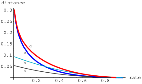
Figure 5. Parameters of expander codes: (a) Bound (3), (b) Bound (22), (c) product (Zyablov) bound, (d) Bound (23).

$R$	0.1	0.2	0.3	0.4	0.5	0.6	0.7	0.8	0.9
$\delta_{\text{Z}}(R)$	0.129	0.073	0.044	0.026	0.015	0.008	0.0040	0.0015	0.00030
improved bound (22)	0.077	0.061	0.046	0.034	0.024	0.015	0.0084	0.0037	0.00089
improved bound (23)	0.148	0.095	0.063	0.041	0.026	0.015	0.0078	0.0031	0.00073

.

It is interesting that an improvement of the product bound is obtained already with the basic construction of Sect. 4.1. Moreover, for large rates this construction gives codes with a distance larger than of the modified bipartite-graph construction of Sect. 4.2. On the other hand, the modified construction asymptotically improves the product bound for all values of the code rate other than $0$ and $1$. Both code families are polynomially constructible.

Concluding this section we remark that in principle, the techniques presented here will generalize to yield an improvement of the bound [6] for codes from hypergraphs.

5. Families of asymptotically good binary codes and their construction complexity

Here we compare the parameters and construction complexity of other asymptotically good families of binary codes with the families of bipartite-graph codes presented in the previous section.

First note that the complexity of specifying the bipartite-graph codes is proportional to the complexity of describing the graph $G$ which is $O(N\log N)$ if the graph is represented by a permutation of the $N$ vertices in any one part. For most Ramanujan graphs, constructing this permutation has complexity not more than $O(N\log N)$. The complexity of constructing codes meeting the Zyablov bound (6) in the traditional way is at most $O(N^{2})$, by a combination of the results in [24, 14].

Codes of distance greater than that given by the Zyablov bound can be constructed as multilevel concatenations [7] or as concatenations of good binary codes of relatively small length with algebraic geometry codes from asymptotically maximal curves [12]. The parameters of multilevel concatenations of order $m$ are given by the following Blokh-Zyablov bounds [7]:

$$R^{(m)}(\delta)=\max_{R_{0}\leq 1-h(\delta)}\Big{\{}R_{0}-\frac{\delta R_{0}}{m}\sum_{i=1}^{m}\Big{[}\delta_{\text{\rm GV}}\Big{(}R_{0}\frac{m-i+1}{m}\Big{)}^{-1}\Big{]}\Big{\}},\quad m=1,2,\dots.$$

(in this case it is more convenient to specify the code rate $R$ for a fixed value of the relative distance $\delta$). Note that for $m=1$ we again obtain (6). The value $R^{(m)}(\delta)$ increases monotonically with $m$ for any $0<\delta<1/2$ and thus these codes surpass the Zyablov bound for all $m\geq 2.$ Their construction complexity is $O(N^{\max(2,(m/R)-1)})$ which is higher than the complexity of constructing the bipartite-graph codes, particularly for low code rates. The bound $R^{(m)}(\delta)$ is better than the value of the rate obtained for bipartite-graph codes beginning with $m=4$ or so.

The largest code rate of multilevel concatenations is obtained by letting $m\to\infty$. The resulting bound is given by

$$R^{(\infty)}(\delta)=1-h(\delta)-\delta\int_{0}^{1-h(\delta)}\frac{dx}{\delta_{\text{\rm GV}}(x)}$$

(this expression is called the Blokh-Zyablov bound).

Concatenations of algebraic-geometry codes with short binary codes introduced in [12] improve the Blokh-Zyablov bound $R^{(\infty)}$ for all $0<\delta<1/2$ (but do not meet the GV bound on the ensemble-average distance of concatenated codes). The code rate of these codes is the largest known asymptotically (for a given $\delta$) among families of binary codes with polynomial construction complexity. The construction complexity of this code family is $O(N^{3}\log^{3}N)$ by a recent result of K. Shum et al. [15].

Perhaps the most important is the fact that even though the two families mentioned above have better parameters than bipartite-graph codes, their designed distance in both cases is estimated by the product bound. On the contrary, the code families constructed in this paper provide an asymptotic improvement of the product bound on the distance.

References

- [1] N. Alon, J. Bruck, M. Naor, J. Naor, and R. Roth, Construction of asymptotically good low-rate error-correcting codes through pseudo-random graphs, IEEE Trans. Inform. Theory 38, no. 2 (1992), 309–315.
- [2] A. Barg, J. Justesen, and C. Thommesen, Concatenated codes with fixed inner code and random outer code, IEEE Trans. Inform. Theory (2001), no. 1, 361–365.
- [3] A. Barg and G. Zémor, Concatenated codes: Serial and parallel, Proc. 2003 IEEE International Sympos. Inform. Theory, Yokohama, Japan, p. 465; submitted to IEEE Trans. Inform. Theory, http://www.infres.enst.fr/ zemor/concatenated.ps.
- [4] by same author, Error exponents of expander codes under linear-complexity decoding, SIAM Journal on Discrete Mathematics 17, no 3 (2004), 426–443.
- [5] by same author, Error exponents of expander codes, IEEE Trans. Inform. Theory 48 (2002), no. 6, 1725–1729.
- [6] Y. Bilu and S. Hoory, On codes from hypergraphs, European Journal of Combinatorics 25 (2004), 339–354.
- [7] E. L. Blokh and V. V. Zyablov, Linear concatenated codes, Nauka, Moscow, 1982, (In Russian).
- [8] J. Boutros, O. Pothier, and G. Zémor, Generalized low density Tanner codes, Proc. IEEE ICC, vol. 1, 1999, pp. 441–445.
- [9] G. D. Forney, Jr., Concatenated codes, MIT Press, Cambridge, MA, 1966.
- [10] R. G. Gallager, Low-density parity-check codes, MIT Press, Cambridge, MA, 1963.
- [11] V. Guruswami and P. Indyk, Near-optimal linear-time codes for unique decoding and new list-decodable codes over smaller alphabets, Proceedings of the ACM Symposium on the Theory of Computing (STOC), 2002, pp. 812–821.
- [12] G. L. Katsman and M. A. Tsfasman, and S. G. Vlăduţ, M̧odular curves and codes with polynomial complexity of construction, IEEE Trans. Inform. Theory, 30 (1984), 353–355.
- [13] M. Lentmaier and K. Sh. Zigangirov, On generalized low-density parity-check codes based on Hamming component codes, IEEE Communications Letters 3 (1999), no. 8, 248–250.
- [14] B.-Z. Shen, A Justesen construction of binary concatenated codes which asymptotically meet Zyablov bound for low rate, IEEE Trans. Inform. Theory, IT-39, no. 1 (1993), 239–242.
- [15] K. W. Shum, I. Aleshnikov, P. V. Kumar, H. Stichtenoth, and V. Deolalikar, A low-complexity algorithm for the construction of algebraic-geometric codes better than the Gilbert-Varshamov bound, IEEE Trans. Inform. Theory, 47, no 6 (2001), pp. 2225–2241.
- [16] M. Sipser and D. A. Spielman, Expander codes, IEEE Trans. Inform. Theory 42 (1996), no. 6, 1710–1722.
- [17] V. Skachek and R. Roth, Generalized minimum distance decoding of expander codes, Proc. IEEE Information Theory Workshop, Paris, France, March 2003.
- [18] by same author, On nearly-MDS expander codes, Proc. 2004 IEEE Internat. Sympos. Inform. Theory, Chicago, IL (2004), p.8.
- [19] R. M. Tanner, A recursive approach to low-complexity codes, IEEE Trans. Inform. Theory 27 (1981), no. 5, 1710–1722.
- [20] R. M. Tanner, Superproduct codes with improved minimum distance Proc. 2002 IEEE International Symposium on Information Theory, p. 283.
- [21] C. Thommesen, The existence of binary linear concatenated codes with Reed-Solomon outer codes which asymptotically meet the Gilbert-Varshamov bound, IEEE Trans. Inform. Theory 29 (1983), 850–853.
- [22] by same author, Error-correcting capabilities of concatenated codes with MDS outer codes on memoryless channels with maximum-likelihood decoding, IEEE Trans. Inform. Theory 33 (1987), no. 5, 632–640.
- [23] G. Zémor, On expander codes, IEEE Trans. Inform. Theory 47 (2001), no. 2, 835–837.
- [24] V. V. Zyablov, An estimate of complexity of constructing binary linear cascade codes, Problems of Information Transmission 7 (1971), no. 1, 3–10.