A measure of similarity between graph vertices: Applications to synonym extraction and web searching

Abstract

We introduce a concept of similarity between vertices of directed graphs. Let $G_{A}$ and $G_{B}$ be two directed graphs with respectively $n_{A}$ and $n_{B}$ vertices. We define a $n_{B}\times n_{A}$ similarity matrix $\mathbf{S}$ whose real entry $s_{ij}$ expresses how similar vertex $j$ (in $G_{A})$ is to vertex $i$ (in $G_{B}$) : we say that $s_{ij}$ is their similarity score. The similarity matrix can be obtained as the limit of the normalized even iterates of $S(k+1)=BS(k)A^{T}+B^{T}S(k)A$ where $A$ and $B$ are adjacency matrices of the graphs and $S(0)$ is a matrix whose entries are all equal to one. In the special case where $G_{A}=G_{B}=G$, the matrix $\mathbf{S}$ is square and the score $s_{ij}$ is the similarity score between the vertices $i$ and $j$ of $G$. We point out that Kleinberg’s “hub and authority” method to identify web-pages relevant to a given query can be viewed as a special case of our definition in the case where one of the graphs has two vertices and a unique directed edge between them. In analogy to Kleinberg, we show that our similarity scores are given by the components of a dominant eigenvector of a non-negative matrix. Potential applications of our similarity concept are numerous. We illustrate an application for the automatic extraction of synonyms in a monolingual dictionary.

1 Generalizing hubs and authorities

Efficient web search engines such as Google are often based on the idea of characterizing the most important vertices in a graph representing the connections or links between pages on the web. One such method, proposed by Kleinberg [18], identifies in a set of pages relevant to a query search the subset of pages that are good hubs or the subset of pages that are good authorities. For example, for the query “university”, the home-pages of Oxford, Harvard and other universities are good authorities, whereas web pages that point to these home-pages are good hubs. Good hubs are pages that point to good authorities, and good authorities are pages that are pointed to by good hubs. From these implicit relations, Kleinberg derives an iterative method that assigns an “authority score” and a “hub score” to every vertex of a given graph. These scores can be obtained as the limit of a converging iterative process which we now describe.

Let $G=(V,E)$ be a graph with vertex set $V$ and with edge set $E$ and let $h_{j}$ and $a_{j}$ be the hub and authority scores of vertex $j$. We let these scores be initialized by some positive values and then update them simultaneously for all vertices according to the following mutually reinforcing relation : the hub score of vertex $j$ is set equal to the sum of the authority scores of all vertices pointed to by $j$ and, similarly, the authority score of vertex $j$ is set equal to the sum of the hub scores of all vertices pointing to $j$ :

$$\left\{\begin{array}[]{rclll}h_{j}&\leftarrow&\sum_{i:(j,i)\in E}a_{i}\\[5.69054pt] a_{j}&\leftarrow&\sum_{i:(i,j)\in E}h_{i}\end{array}\right.$$

Let $B$ be the matrix whose entry $(i,j)$ is equal to the number of edges between the vertices $i$ and $j$ in $G$ (the adjacency matrix of $G$), and let $h$ and $a$ be the vectors of hub and authority scores. The above updating equations then take the simple form

$$\left[\begin{array}[]{c}h\\ a\end{array}\right]_{k+1}=\left[\begin{array}[]{cc}0&B\\ B^{T}&0\end{array}\right]\left[\begin{array}[]{c}h\\ a\end{array}\right]_{k},\qquad k=0,1,\ldots$$

which we denote in compact form by

$$x_{k+1}=M\;x_{k},\qquad k=0,1,\ldots$$

where

$$x_{k}=\left[\begin{array}[]{c}h\\ a\end{array}\right]_{k},\quad M=\left[\begin{array}[]{cc}0&B\\ B^{T}&0\end{array}\right].$$

Notice that the matrix $M$ is symmetric and non-negative. We are only interested in the relative scores and we will therefore consider the normalized vector sequence

$$z_{0}=x_{0}>0,\quad z_{k+1}=\frac{Mz_{k}}{\|Mz_{k}\|_{2}},\quad k=0,1,\ldots$$ (1)

where $\|\cdot\|_{2}$ is the Euclidean vector norm. Ideally, we would like to take the limit of the sequence $z_{k}$ as a definition for the hub and authority scores. There are two difficulties with such a definition.

A first difficulty is that the sequence $z_{k}$ does not always converge. In fact, sequences associated with non-negative matrices $M$ with the above block structure almost never converge but rather oscillate between the limits

$$z_{even}=\lim_{k\rightarrow\infty}z_{2k}\quad\mbox{ and }\quad z_{odd}=\lim_{k\rightarrow\infty}z_{2k+1}.$$

We prove in Theorem 2 that this is true in general for symmetric non-negative matrices, and that either the sequence resulting from (1) converges, or it doesn’t and then the even and odd sub-sequences do converge. Let us consider both limits for the moment.

The second difficulty is that the limit vectors $z_{even}$ and $z_{odd}$ do in general depend on the initial vector $z_{0}$ and there is no apparently natural choice for $z_{0}$. The set of all limit vectors obtained when starting from a positive initial vector is given by

$$Z=\{z_{even}(z_{0}),z_{odd}(z_{0}):z_{0}>0\}$$

and we would like to select one particular vector in that set. The vector $z_{even}$ obtained for $z_{0}={\bf 1}$ (we denote by ${\bf 1}$ the vector, or matrix, whose entries are all equal to 1) has several interesting features that qualifies it as a good choice: it is particularly easy to compute, it possesses several nice properties (see in particular Section 4), and it has the extremal property, proved in Theorem 2, of being the unique vector in $Z$ of largest possible 1-norm (the 1-norm of a vector is the sum of all the magnitudes of its entries). Because of these features, we take the two sub-vectors of $z_{even}({\bf 1})$ as definitions for the hub and authority scores. In the case of the above matrix $M$, we have

$$M^{2}=\left[\begin{array}[]{cc}BB^{T}&0\\ 0&B^{T}B\end{array}\right]$$

and from this equality it follows that, if the dominant invariant subspaces associated with $BB^{T}$ and $B^{T}B$ have dimension one, then the normalized hub and authority scores are simply given by the normalized dominant eigenvectors of $BB^{T}$ and $B^{T}B$. This is the definition used in [18] for the authority and hub scores of the vertices of $G$. The arbitrary choice of $z_{0}={\bf 1}$ made in [18] is shown here to have an extremal norm justification. Notice that when the invariant subspace has dimension one, then there is nothing particular about the starting vector ${\bf 1}$ since any other positive vector $z_{0}$ would give the same result.

We now generalize this construction. The authority score of vertex $j$ of $G$ can be thought of as a similarity score between vertex $j$ of $G$ and vertex authority of the graph

$$hub\longrightarrow authority$$

and, similarly, the hub score of vertex $j$ of $G$ can be seen as a similarity score between vertex $j$ and vertex hub. The mutually reinforcing updating iteration used above can be generalized to graphs that are different from the hub-authority structure graph. The idea of this generalization is easier to grasp with an example; we illustrate it first on the path graph with three vertices and then provide a definition for arbitrary graphs. Let $G$ be a graph with edge set $E$ and adjacency matrix $B$ and consider the structure graph

$$1\longrightarrow 2\longrightarrow 3.$$

With each vertex $j$ of $G$ we now associate three scores $x_{i1},x_{i2}$ and $x_{i3}$; one for each vertex of the structure graph. We initialize these scores with some positive value and then update them according to the following mutually reinforcing relation

$$\left\{\begin{array}[]{rclll}x_{i1}&\leftarrow&&\sum_{j:(i,j)\in E}x_{i2}\\[5.69054pt] x_{i2}&\leftarrow&\sum_{j:(j,i)\in E}x_{i1}&&+\sum_{j:(i,j)\in E}x_{i3}\\[5.69054pt] x_{i3}&\leftarrow&&\sum_{j:(j,i)\in E}x_{i2}\end{array}\right.$$

or, in matrix form (we denote by $\mathbf{x}_{j}$ the column vector with entries $x_{ij}$),

$$\left[\begin{array}[]{c}\mathbf{x}_{1}\\ \mathbf{x}_{2}\\ \mathbf{x}_{3}\end{array}\right]_{k+1}=\left[\begin{array}[]{ccc}0&B&0\\ B^{T}&0&B\\ 0&B^{T}&0\end{array}\right]\left[\begin{array}[]{c}\mathbf{x}_{1}\\ \mathbf{x}_{2}\\ \mathbf{x}_{3}\end{array}\right]_{k},\qquad k=0,1,\ldots$$

which we again denote by $x_{k+1}=Mx_{k}$. The situation is now identical to that of the previous example and all convergence arguments given there apply here as well. The matrix $M$ is symmetric and non-negative, the normalized even and odd iterates converge and the limit $z_{even}({\bf 1})$ is among all possible limits the unique vector with largest possible 1-norm. We take the three components of this extremal limit $z_{even}({\bf 1})$ as definition for the similarity scores $s_{1},s_{2}$ and $s_{3}$ and define the similarity matrix by ${\bf S}=[s_{1}\;s_{2}\;s_{3}]$. A numerical example of such a similarity matrix is shown in Figure 1. Note that we shall prove in Theorem 6 that the score $s_{2}$ can be obtained more directly from $B$ by computing the dominating eigenvector of the matrix $BB^{T}+B^{T}B$.

$\left[\begin{array}[]{ccc}0.3160&0.1460&0\\ \vskip 6.0pt plus 2.0pt minus 2.0pt\cr 0.1990&0.5540&0.0610\\ \vskip 6.0pt plus 2.0pt minus 2.0pt\cr 0.0610&0.5540&0.1990\\ \vskip 6.0pt plus 2.0pt minus 2.0pt\cr 0.1580&0.0680&0.1580\\ \vskip 6.0pt plus 2.0pt minus 2.0pt\cr 0&0.1460&0.3160\end{array}\right]$

Fig. 1: A graph and its similarity matrix with the structure graph $1\longrightarrow 2\longrightarrow 3$. The similarity score of vertex 3 with vertex 2 of the structure graph is equal to 0.5540.

We now come to a description of the general case. Assume that we have two directed graphs $G_{A}$ and $G_{B}$ with $n_{A}$ and $n_{B}$ vertices and edge sets $E_{A}$ and $E_{B}$. We think of $G_{A}$ as a structure graph that plays the role of the graphs $hub\longrightarrow authority$ and $1\longrightarrow 2\longrightarrow 3$ in the above examples. We consider real scores $x_{ij}$ for $i=1,\ldots,n_{B}$ and $j=1,\ldots,n_{A}$ and simultaneously update all scores according to the following updating equations

$$x_{ij}\;\leftarrow\sum_{r:(r,i)\in E_{B},\;s:(s,j)\in E_{A}}x_{rs}+\sum_{r:(i,r)\in E_{B},\;s:(j,s)\in E_{A}}x_{rs}.$$

This equation can be given an interpretation in terms of the product graph of $G_{A}$ and $G_{B}$. The product graph of $G_{A}$ and $G_{B}$ is a graph that has $n_{A}.n_{B}$ vertices and that has an edge between vertices $(i_{1},j_{1})$ and $(i_{2},j_{2})$ if there is an edge between $i_{1}$ and $i_{2}$ in $G_{A}$ and there is an edge between $j_{1}$ and $j_{2}$ in $G_{B}$. The updating equation (1) is then equivalent to replacing the values of all vertices of the product graph by the values of the outgoing and incoming vertices in the graph.

Equation (1) can also be written in more compact matrix form. Let $X_{k}$ be the $n_{B}\times n_{A}$ matrix of entries $x_{ij}$ at iteration $k$. Then the updating equations take the simple form

$$X_{k+1}=BX_{k}A^{T}+B^{T}X_{k}A,\qquad k=0,1,\ldots$$ (2)

where $A$ and $B$ are the adjacency matrices of $G_{A}$ and $G_{B}$. We prove in Section 3 that, as for the above examples, the normalized even and odd iterates of this updating equation converge, and that the limit $Z_{even}({\bf 1})$ is among all possible limits the only one with largest 1-norm. We take this limit as definition of the similarity matrix. An example of two graphs and their similarity matrix is shown in Figure 2.

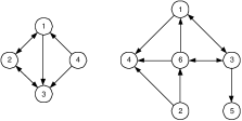
$\left[\begin{array}[]{cccc}0.2720&0.2840&0.2700&0.1440\\ \vskip 6.0pt plus 2.0pt minus 2.0pt\cr 0.1400&0.1390&0.0670&0.1390\\ \vskip 6.0pt plus 2.0pt minus 2.0pt\cr 0.2700&0.3120&0.2560&0.1650\\ \vskip 6.0pt plus 2.0pt minus 2.0pt\cr 0.2300&0.2440&0.2870&0.0720\\ \vskip 6.0pt plus 2.0pt minus 2.0pt\cr 0.0660&0.0720&0.1030&0\\ \vskip 6.0pt plus 2.0pt minus 2.0pt\cr 0.2540&0.2480&0.2340&0.1460\end{array}\right]$

Fig. 2: Two graphs $G_{A},G_{B}$ and their similarity matrix. The vertex of $G_{A}$ which is most similar to vertex 5 in $G_{B}$ is vertex $3$.

It is interesting to note that in the database literature similar ideas have been proposed [20], [17]. The applications there are information retrieval in large databases with which a particular graph structure can be associated. The ideas presented in these conference papers are obviously linked to those of the present paper, but in order to guarantee convergence of the proposed iteration to a unique fixed point, the iteration has to be slightly modified using e.g. certain weighting coefficients. Therefore, the hub and authority score of Kleinberg is not a special case of their definition. We thank the authors of [17] for drawing our attention to those references.

The rest of this paper is organized as follows. In Section 2, we describe some standard Perron-Frobenius results for non-negative matrices that are useful in the rest of the paper. In Section 3, we give a precise definition of the similarity matrix together with different alternative definitions. The definition immediately translates into an approximation algorithm and we discuss in that section some complexity aspects of the algorithm. In Section 4 we describe similarity matrices for the situation where one of the two graphs is a path graph of length 2 or 3. In Section 5 we consider the special case $G_{A}=G_{B}=G$ for which the score $s_{ij}$ is the similarity between the vertices $i$ and $j$ in a single graph $G$. Section 6 deals with graphs whose similarity matrix have rank one. We prove there that if one of the graphs is regular or if one of the graphs is undirected, then the similarity matrix has rank one. Regular graphs are graphs whose vertices have the same in-degrees, and the same out-degrees; cycle graphs, for example, are regular. In a final section we report results obtained for the automatic synonym extraction in a dictionary by using the central score of a graph. A short version of this paper appears as a conference contribution in [6].

2 Graphs and non-negative matrices

With any directed graph $G=(V,E)$ one can an associate a non-negative matrix via an indexation of its vertices. The so-called adjacency matrix of $G$ is the matrix $B\in{\mathbb{N}}^{n\times n}$ whose entry $b_{ij}$ equals the number of edges from vertex $i$ to vertex $j$. Let $B$ be the adjacency matrix of some graph $G$; the entry $(B^{k})_{ij}$ is equal to the number of paths of length $k$ from vertex $i$ to vertex $j$. From this it follows that a graph is strongly connected if and only if for every pair of indices $i$ and $j$ there is an integer $k$ such that $(B^{k})_{ij}>0$. Matrices that satisfy this property are said to be irreducible.

In the sequel, we shall need the notion of orthogonal projection on vector subspaces. Let $\mathcal{V}$ be a linear subspace of $\mathbb{R}^{n}$ and let $v\in\mathbb{R}^{n}$. The orthogonal projection of $v$ on $\mathcal{V}$ is the vector in $\mathcal{V}$ with smallest Euclidean distance to $v$. A matrix representation of this projection can be obtained as follows. Let $\{v_{1},\ldots,v_{m}\}$ be an orthonormal basis for $\mathcal{V}$ and arrange the column vectors $v_{i}$ in a matrix $V$. The projection of $v$ on $\mathcal{V}$ is then given by $\Pi v=VV^{T}v$ and the matrix $\Pi=VV^{T}$ is the orthogonal projector on $\mathcal{V}$. Projectors have the property that $\Pi^{2}=\Pi$.

The Perron-Frobenius theory [14] establishes interesting properties about the eigenvectors and eigenvalues for non-negative matrices. Let the largest magnitude of the eigenvalues of the matrix $M$ (the spectral radius of $M$) be denoted by $\rho(M)$. According to the Perron-Frobenius Theorem, the spectral radius of a non-negative matrix $M$ is an eigenvalue of $M$ (called the Perron root), and there exists an associated non-negative vector $x\geq 0$ ($x\neq 0$) such that $Mx=\rho x$ (called the Perron vector). In the case of symmetric matrices, more specific results can be obtained.

Theorem 1.

Let $M$ be a symmetric non-negative matrix of spectral radius $\rho$. Then the algebraic and geometric multiplicity of the Perron root $\rho$ are equal; there is a non-negative basis $X\geq 0$ for the invariant subspace associated with the Perron root; and the elements of the orthogonal projector $\Pi$ on the vector space associated with the Perron root of $M$ are all non-negative.

Proof.

We use the facts that any symmetric non-negative matrix $M$ can be permuted to a block-diagonal matrix with irreducible blocks $M_{i}$ on the diagonal [14, 3], and that the algebraic multiplicity of the Perron root of an irreducible non-negative matrix is equal to one. From these combined facts it follows that the algebraic and geometric multiplicities of the Perron root $\rho$ of $M$ are equal. Moreover, the corresponding invariant subspace of $M$ is obtained from the normalized Perron vectors of the $M_{i}$ blocks, appropriately padded with zeros. The basis $X$ one obtains that way is then non-negative and orthonormal. ∎

The next theorem will be used to justify our definition of similarity matrix between two graphs. The result describes the limit vectors of sequences associated with symmetric non-negative linear transformations.

Theorem 2.

Let $M$ be a symmetric non-negative matrix of spectral radius $\rho$. Let $z_{0}>0$ and consider the sequence

$$z_{k+1}=Mz_{k}/\|Mz_{k}\|_{2},\quad k=0,\ldots$$

Two convergence cases can occur depending on whether or not $-\rho$ is an eigenvalue of $M$. When $-\rho$ is not an eigenvalue of $M$, then the sequence $z_{k}$ simply converges to ${\Pi z_{0}}/{\|\Pi z_{0}\|_{2}}$, where $\Pi$ is the orthogonal projector on the invariant subspace associated with the Perron root $\rho$. When $-\rho$ is an eigenvalue of $M$, then the subsequences $z_{2k}$ and $z_{2k+1}$ converge to the limits

$$z_{even}(z_{0})=\lim_{k\rightarrow\infty}z_{2k}=\frac{\Pi z_{0}}{\|\Pi z_{0}\|_{2}}\quad\mbox{ and }\quad z_{odd}(z_{0})=\lim_{k\rightarrow\infty}z_{2k+1}=\frac{\Pi Mz_{0}}{\|\Pi Mz_{0}\|_{2}},$$

where $\Pi$ is the orthogonal projector on the sums of the invariant subspaces associated with $\rho$ and $-\rho$. In both cases the set of all possible limits is given by

$$Z=\{z_{even}(z_{0}),z_{odd}(z_{0}):z_{0}>0\}=\{\Pi z/\|\Pi z\|_{2}:z>0\}$$

and the vector $z_{even}({\bf 1})$ is the unique vector of largest possible 1-norm in that set.

Proof.

We prove only the case where $-\rho$ is an eigenvalue; the other case is a trivial modification. Let us denote the invariant subspaces of $M$ corresponding to $\rho$, to $-\rho$ and to the rest of the spectrum, respectively by $\mathcal{V}_{\rho}$, $\mathcal{V}_{-\rho}$ and $\mathcal{V}_{\mu}$. Assume that these spaces are non-trivial, and that we have orthonormal bases for them :

$$MV_{\rho}=\rho V_{\rho},\quad MV_{-\rho}=-\rho V_{-\rho},\quad MV_{\mu}=V_{\mu}M_{\mu},$$

where $M_{\mu}$ is a square matrix (diagonal if $V_{\mu}$ is the basis of eigenvectors) with spectral radius $\mu$ strictly less than $\rho$. The eigenvalue decomposition can then be rewritten in block diagonal form :

$$\begin{array}[]{rcl}M&=&\left[\begin{array}[]{ccc}V_{\rho}&V_{-\rho}&V_{\mu}\end{array}\right]\left[\begin{array}[]{ccc}\rho I&&\\ &-\rho I&\\ &&M_{\mu}\end{array}\right]\left[\begin{array}[]{ccc}V_{\rho}&V_{-\rho}&V_{\mu}\end{array}\right]^{T}\\ &=&\rho V_{\rho}V_{\rho}^{T}-\rho V_{-\rho}V_{-\rho}^{T}+V_{\mu}M_{\mu}V_{\mu}^{T}.\end{array}$$

It then follows that

$$M^{2}=\rho^{2}\Pi+V_{\mu}M_{\mu}^{2}V_{\mu}^{T}$$

where $\Pi:=V_{\rho}V_{\rho}^{T}+V_{-\rho}V_{-\rho}^{T}$ is the orthogonal projector onto the invariant subspace $\mathcal{V}_{\rho}\oplus\mathcal{V}_{-\rho}$ of $M^{2}$ corresponding to $\rho^{2}$. We also have

$$M^{2k}=\rho^{2k}\Pi+V_{\mu}M_{\mu}^{2k}V_{\mu}^{T}$$

and since $\rho(M_{\mu})=\mu<\rho$, it follows from multiplying this by $z_{0}$ and $Mz_{0}$ that

$$z_{2k}=\frac{\Pi z_{0}}{\|\Pi z_{0}\|_{2}}+O(\mu/\rho)^{2k}$$

and

$$z_{2k+1}=\frac{\Pi Mz_{0}}{\|\Pi Mz_{0}\|_{2}}+O(\mu/\rho)^{2k}$$

provided the initial vectors $z_{0}$ and $Mz_{0}$ have a non-zero component in the relevant subspaces, i.e. provided $\Pi z_{0}$ and $\Pi Mz_{0}$ are non-zero. But the Euclidean norm of these vectors equal $z_{0}^{T}\Pi z_{0}$ and $z_{0}^{T}M\Pi Mz_{0}$ since $\Pi^{2}=\Pi$. These norms are both non-zero since $z_{0}>0$ and both $\Pi$ and $M\Pi M$ are non-negative and non-zero.

It follows from the non-negativity of $M$ and the formula for $z_{even}(z_{0})$ and $z_{odd}(z_{0})$ that both limits lie in $\{\Pi z/\|\Pi z\|_{2}:z>0\}$. Let us now show that every element $\hat{z}_{0}\in\{\Pi z/\|\Pi z\|_{2}:z>0\}$ can be obtained as $z_{even}(z_{0})$ for some $z_{0}>0$. Since the entries of $\Pi$ are non-negative, so are those of $\hat{z}_{0}$. This vector may however have some of its entries equal to zero. From $\hat{z}_{0}$ we construct $z_{0}$ by adding $\epsilon$ to all the zero entries of $\hat{z}_{0}$. The vector $z_{0}-\hat{z}_{0}$ is clearly orthogonal to $\mathcal{V}_{\rho}\oplus\mathcal{V}_{-\rho}$ and will therefore vanish in the iteration of $M^{2}$. Thus we have $z_{even}(z_{0})=\hat{z}_{0}$ for $z_{0}>0$, as requested.

We now prove the last statement. The matrix $\Pi$ and all vectors are non-negative and $\Pi^{2}=\Pi$, and so,

$$\left|\left|\frac{\Pi{\mathbf{1}}}{\|\Pi{\mathbf{1}}\|_{2}}\right|\right|_{1}=\sqrt{{\mathbf{1}}^{T}\Pi^{2}{\mathbf{1}}}$$

and also

$$\left|\left|\frac{\Pi{z_{0}}}{\|\Pi{z_{0}}\|_{2}}\right|\right|_{1}=\frac{{\mathbf{1}}^{T}\Pi^{2}{z_{0}}}{\sqrt{{z_{0}}^{T}\Pi^{2}{z_{0}}}}.$$

Applying the Schwarz inequality to $\Pi z_{0}$ and $\Pi{\mathbf{1}}$ yields

$$|{\mathbf{1}}^{T}\Pi^{2}z_{0}|\leq\sqrt{z_{0}^{T}\Pi^{2}z_{0}}.\sqrt{{\mathbf{1}}^{T}\Pi^{2}{\mathbf{1}}}.$$

with equality only when $\Pi z_{0}=\lambda\Pi{\mathbf{1}}$ for some $\lambda\in\C$. But since $\Pi z_{0}$ and $\Pi{\mathbf{1}}$ are both real non-negative, the proof easily follows. ∎

3 Similarity between vertices in graphs

We now come to a formal definition of the similarity matrix of two directed graphs $G_{A}$ and $G_{B}$. The updating equation for the similarity matrix is motivated in the introduction and is given by the linear mapping:

$$X_{k+1}=BX_{k}A^{T}+B^{T}X_{k}A,\qquad k=0,1,\ldots$$ (3)

where $A$ and $B$ are the adjacency matrices of $G_{A}$ and $G_{B}$. In this updating equation, the entries of $X_{k+1}$ depend linearly on those of $X_{k}$. We can make this dependance more explicit by using the matrix-to-vector operator that develops a matrix into a vector by taking its columns one by one. This operator, denoted ${\rm{vec}}$, satisfies the elementary property ${\rm{vec}}(CXD)=(D^{T}\otimes C)\;{\rm{vec}}(X)$ in which $\otimes$ denotes the Kronecker product (also denoted tensorial, direct or categorial product). For a proof of this property, see Lemma 4.3.1 in [15]. Applying this property to (3) we immediately obtain

$$x_{k+1}=(A\otimes B+A^{T}\otimes B^{T})\;x_{k}$$ (4)

where $x_{k}={\rm{vec}}(X_{k})$. This is the format used in the introduction. Combining this observation with Theorem 2 we deduce the following theorem.

Theorem 3.

Let $G_{A}$ and $G_{B}$ be two graphs with adjacency matrices $A$ and $B$, fix some initial positive matrix $Z_{0}>0$ and define

$$Z_{k+1}=\frac{BZ_{k}A^{T}+B^{T}Z_{k}A}{\|BZ_{k}A^{T}+B^{T}Z_{k}A\|_{F}}\qquad k=0,1,\ldots.$$

Then, the matrix subsequences $Z_{2k}$ and $Z_{2k+1}$ converge to $Z_{even}$ and $Z_{odd}.$ Moreover, among all the matrices in the set

$$\{Z_{even}(Z_{0}),Z_{odd}(Z_{0}):Z_{0}>0\}$$

the matrix $Z_{even}({\bf 1})$ is the unique matrix of largest 1-norm.

In order to be consistent with the vector norm appearing in Theorem 2, the matrix norm $\|.\|_{F}$ we use here is the square root of the sum of all squared entries (this norm is known as the Euclidean or Frobenius norm), and the 1-norm $\|.\|_{1}$ is the sum of the magnitudes of all its entries. One can also provide a definition of the set $Z$ in terms of one of its extremal properties.

Theorem 4.

Let $G_{A}$ and $G_{B}$ be two graphs with adjacency matrices $A$ and $B$ and consider the notation of Theorem 3. The set

$$Z=\{Z_{even}(Z_{0}),Z_{odd}(Z_{0}):Z_{0}>0\}$$

and the set of all positive matrices that maximize the expression

$$\frac{\|BXA^{T}+B^{T}XA\|_{F}}{\|X\|_{F}}.$$

are equal. Moreover, among all matrices in this set there is a unique matrix $\mathbf{S}$ whose 1-norm is maximal. This matrix can be obtained as

$$\mathbf{S}=\lim_{k\rightarrow+\infty}Z_{2k}$$

for $Z_{0}={\bf 1}$.

Proof.

The above expression can also be written as $\|L(X)\|_{2}/\|X\|_{2}$ which is the induced 2-norm of the linear mapping $L$ defined by $L(X)=BXA^{T}+B^{T}XA$. It is well known [14] that each dominant eigenvector $X$ of ${L}^{2}$ is a maximizer of this expression. It was shown above that ${\mathbf{S}}$ is the unique matrix of largest 1-norm in that set. ∎

We take the matrix $\mathbf{S}$ appearing in this Theorem as definition of similarity matrix between $G_{A}$ and $G_{B}$. Notice that it follows from this definition that the similarity matrix between $G_{B}$ and $G_{A}$ is the transpose of the similarity matrix between $G_{A}$ and $G_{B}$.

A direct algorithmic transcription of the definition leads to an approximation algorithm for computing similarity matrices of graphs:

1. Set $Z_{0}={\bf 1}$.

2. Iterate an even number of times

$$Z_{k+1}=\frac{BZ_{k}A^{T}+B^{T}Z_{k}A}{\|BZ_{k}A^{T}+B^{T}Z_{k}A\|_{F}}$$

and stop upon convergence of $Z_{k}$.

4. Output $\mathbf{S}$.

This algorithm is a matrix analog to the classical power method (see [14]) to compute a dominant eigenvector of a matrix. The complexity of this algorithm is easy to estimate. Let $G_{A},G_{B}$ be two graphs with $n_{A},n_{B}$ vertices and $e_{A},e_{B}$ edges, respectively. Then the products $BZ_{k}$ and $B^{T}Z_{k}$ require less than $2n_{A}.e_{B}$ additions and multiplications each, while the subsequent products $(BZ_{k})A^{T}$ and $(B^{T}Z_{k})A$ require less than $2n_{B}.e_{A}$ additions and multiplications each. The sum and the calculation of the Frobenius norm requires $2n_{A}.n_{B}$ additions and multiplications, while the scaling requires one division and $n_{A}.n_{B}$ multiplications. Let us define

$$\alpha_{A}:=e_{A}/n_{A},\quad\alpha_{B}:=e_{B}/n_{B}$$

as the average number of non-zero elements per row of $A$ and $B$, respectively, then the total complexity per iteration step is of the order of $4(\alpha_{A}+\alpha_{B})n_{A}n_{B}$ additions and multiplications. As was shown in Theorem 2, the convergence of the even iterates of the above recurrence is linear with ratio $(\mu/\rho)^{2}$. The number of floating point operations needed to compute $\mathbf{S}$ to $\epsilon$ accuracy with the power method is therefore of the order of

$$8n_{A}n_{B}\frac{(\alpha_{A}+\alpha_{B})\log\epsilon}{(\log\mu-\log\rho)}.$$

Other sparse matrix methods could be used here, but we do not address such algorithmic aspects in this paper. For particular classes of adjacency matrices, one can compute the similarity matrix $\mathbf{S}$ directly from the dominant invariant subspaces of matrices of the size of $A$ or $B$. We provide explicit expressions for a few such classes in the next section.

4 Hubs, authorities and central scores

As explained in the introduction, the hub and authority scores of a graph can be expressed in terms of its adjacency matrix.

Theorem 5.

Let $B$ be the adjacency matrix of the graph $G_{B}$. The normalized hub and authority scores of the vertices of $G_{B}$ are given by the normalized dominant eigenvectors of the matrices $BB^{T}$ and $B^{T}B$, provided the corresponding Perron root is of multiplicity 1. Otherwise, it is the normalized projection of the vector ${\mathbf{1}}$ on the respective dominant invariant subspaces.

The condition on the multiplicity of the Perron root is not superfluous. Indeed, even for connected graphs, $BB^{T}$ and $B^{T}B$ may have multiple dominant roots: for cycle graphs for example, both $BB^{T}$ and $B^{T}B$ are the identity matrix.

Another interesting structure graph is the path graph of length three:

$$1\longrightarrow 2\longrightarrow 3$$

As for the hub and authority scores, we can give an explicit expression for the similarity score with vertex $2$, a score that we will call the central score. This central score has been successfully used for the purpose of automatic extraction of synonyms in a dictionary. This application is described in more details in Section 7.

Theorem 6.

Let $B$ be the adjacency matrix of the graph $G_{B}$. The normalized central scores of the vertices of $G_{B}$ are given by the normalized dominant eigenvector of the matrix $B^{T}B+BB^{T}$, provided the corresponding Perron root is of multiplicity 1. Otherwise, it is the normalized projection of the vector ${\mathbf{1}}$ on the dominant invariant subspace.

Proof.

The corresponding matrix $M$ is as follows :

$$M=\left[\begin{array}[]{ccc}0&B&0\\ B^{T}&0&B\\ 0&B^{T}&0\end{array}\right]$$

and so

$$M^{2}=\left[\begin{array}[]{ccc}BB^{T}&0&BB\\ 0&B^{T}B+BB^{T}&0\\ B^{T}B^{T}&0&B^{T}B\end{array}\right]$$

and the result then follows from the definition of the similarity scores, provided the central matrix $B^{T}B+BB^{T}$ has a dominant root $\rho^{2}$ of $M^{2}$. This can be seen as follows. The matrix $M$ can be permuted to

$$M=P^{T}\left[\begin{array}[]{cc}0&E\\ E^{T}&0\end{array}\right]P,\quad\mbox{\rm where }E:=\left[\begin{array}[]{c}B\\ B^{T}\end{array}\right]$$

Let now $V$ and $U$ be orthonormal bases for the dominant right and left singular subspaces of $E$ [14] :

$$EV=\rho U,\quad E^{T}U=\rho V,$$ (5)

then clearly $V$ and $U$ are also bases for the dominant invariant subspaces of $E^{T}E$ and $EE^{T}$, respectively, since

$$E^{T}EV=\rho^{2}V,\quad EE^{T}U=\rho^{2}U.$$

Moreover,

$$PM^{2}P^{T}=\left[\begin{array}[]{cc}EE^{T}&0\\ 0&E^{T}E\end{array}\right]$$

and the projectors associated to the dominant eigenvalues of $EE^{T}$ and $E^{T}E$ are respectively $\Pi_{v}:=VV^{T}$ and $\Pi_{u}:=UU^{T}$. The projector $\Pi$ of $M^{2}$ is then nothing but $P^{T}diag\{\Pi_{v},\Pi_{u}\}P$ and hence the sub-vectors of $\Pi\mathbf{1}$ are the vectors $\Pi_{v}{\mathbf{1}}$ and $\Pi_{u}{\mathbf{1}}$, which can be computed from the smaller matrices $E^{T}E$ or $EE^{T}$. Since $E^{T}E=B^{T}B+BB^{T}$ the central vector $\Pi_{v}{\mathbf{1}}$ is the middle vector of $\Pi{\mathbf{1}}$. It is worth pointing out that (5) also yields a relation between the two smaller projectors :

$$\rho^{2}\Pi_{v}=E^{T}\Pi_{u}E,\quad\rho^{2}\Pi_{u}=E\Pi_{v}E^{T}.$$

∎

In order to illustrate that path graphs of length 3 may have an advantage over the hub-authority structure graph we consider here the special case of the “directed bow-tie graph” $G_{B}$ represented in Figure 3. If we label the center vertex first, then label the $m$ left vertices and finally the $n$ right vertices, the adjacency matrix for this graph is given by

$$B=\left[\begin{array}[]{c|c|c}0&0\;\cdots\;0&1\;\cdots\;1\\ \hline\cr 1&&\\ \vdots&\mathbf{0}_{n}&\mathbf{0}\\ 1&&\\ \hline\cr 0&&\\ \vdots&\mathbf{0}&\mathbf{0}_{m}\\ 0&&\end{array}\right]$$

The matrix $B^{T}B+BB^{T}$ is equal to

$$B^{T}B+BB^{T}=\left[\begin{array}[]{ccc}m+n&0&0\\ 0&\mathbf{1}_{n}&0\\ 0&0&\mathbf{1}_{m}\end{array}\right],$$

and, following Theorem 6, the Perron root of $M$ is equal to $\rho=\sqrt{n+m}$ and the similarity matrix is given by the $(1+m+n)\times 3$ matrix

$$\mathbf{S}=\frac{1}{\sqrt{2(n+m)}}\left[\begin{array}[]{c|c|c}0&\sqrt{n+m}&0\\ \hline\cr 1&0&0\\ \vdots&\vdots&\vdots\\ 1&0&0\\ \hline\cr 0&0&1\\ \vdots&\vdots&\vdots\\ 0&0&1\end{array}\right].$$

This result holds irrespective of the relative value of $m$ and $n$. Let us call the three vertices of the path graph, 1, center and 3, respectively. One could view a center as a vertex through which much information is passed on. This similarity matrix $\mathbf{S}$ indicates that vertex 1 of $G_{B}$ looks very much like a center, the left vertices of $G_{B}$ look like 1’s, and the right vertices of $G_{B}$ look like 3’s. If on the other hand we analyze the graph $G_{B}$ with the hub-authority structure graph of Kleinberg, then the similarity scores $\mathbf{S}$ differ for $m<n$ and $m>n$ :

$$\mathbf{S}_{m>n}=\frac{1}{\sqrt{m+1}}\left[\begin{array}[]{c|c}1&0\\ \hline\cr 0&0\\ \vdots&\vdots\\ 0&0\\ \hline\cr 0&1\\ \vdots&\vdots\\ 0&1\end{array}\right],\quad\mathbf{S}_{m<n}=\frac{1}{\sqrt{n+1}}\left[\begin{array}[]{c|c}0&1\\ \hline\cr 1&0\\ \vdots&\vdots\\ 1&0\\ \hline\cr 0&0\\ \vdots&\vdots\\ 0&0\end{array}\right].$$

This shows a weakness of this structure graph, since the vertices of $G_{B}$ that deserve the label of hub or authority completely change between $m>n$ and $m<n$.

Fig. 3: A directed bow-tie graph. Kleinberg’s hub score of the center vertex is equal to $1/\sqrt{2}$ if $m>n$ and to $0$ if $m<n$. The central score of this vertex is equal to $1/\sqrt{2}$ independently of the relative values of $m$ and $n$.

5 Self-similarity matrix of a graph

When we compare two equal graphs $G_{A}=G_{B}=G$, the similarity matrix $\mathbf{S}$ is a square matrix whose entries are similarity scores between vertices of $G$; this matrix is the self-similarity matrix of $G$. Various graphs and their corresponding self-similarity matrices are represented in Figure 4. In general, we expect vertices to have a high similarity score with themselves; that is, we expect the diagonal entries of self-similarity matrices to be large. We prove in the next theorem that the largest entry of a self-similarity matrix always appears on the diagonal and that, except for trivial cases, the diagonal elements of a self-similarity matrix are non-zero. As can be seen from elementary examples, it is however not true that diagonal elements always dominate all elements on the same row and column.

	$\left[\begin{array}[]{ccc}0.408&0&0\\ \vskip 6.0pt plus 2.0pt minus 2.0pt\cr 0&0.816&0\\ \vskip 6.0pt plus 2.0pt minus 2.0pt\cr 0&0&0.408\end{array}\right]$
	$\left[\begin{array}[]{cccc}0.250&0.250&0.250&0.250\\ \vskip 6.0pt plus 2.0pt minus 2.0pt\cr 0.250&0.250&0.250&0.250\\ \vskip 6.0pt plus 2.0pt minus 2.0pt\cr 0.250&0.250&0.250&0.250\\ \vskip 6.0pt plus 2.0pt minus 2.0pt\cr 0.250&0.250&0.250&0.250\end{array}\right]$
	$\left[\begin{array}[]{cccc}0.182&0&0&0\\ \vskip 6.0pt plus 2.0pt minus 2.0pt\cr 0&0.912&0&0\\ \vskip 6.0pt plus 2.0pt minus 2.0pt\cr 0&0&0.182&0.182\\ \vskip 6.0pt plus 2.0pt minus 2.0pt\cr 0&0&0.182&0.182\end{array}\right]$

Fig. 4: Graphs and their corresponding self-similarity matrix. The self-similarity matrix of a graph gives a measure of how similar vertices are to each other.

Theorem 7.

The self-similarity matrix of a graph is positive semi-definite. In particular, the largest element of the matrix appears on diagonal, and if a diagonal entry is equal to zero the corresponding row and column are equal to zero.

Proof.

Since $A=B$, the iteration of the normalized matrices $Z_{k}$ now becomes

$$Z_{k+1}=\frac{AZ_{k}A^{T}+A^{T}Z_{k}A}{\|AZ_{k}A^{T}+A^{T}Z_{k}A\|_{F}},\quad Z_{0}={\bf 1}.$$

Since the scaled sum of two positive semi-definite matrices is also positive semi-definite, it is clear that all matrices $Z_{k}$ will be positive semi-definite. Moreover, positive semi-definite matrices are a closed set and hence the limit $\mathbf{S}$ will also be positive semi-definite. The properties mentioned in the statement of the theorem are well known properties of positive semi-definite matrices. ∎

When vertices of a graph are similar to each other, such as in cycle graphs, we expect to have a self-similarity matrix with all entries equal. This is indeed the case as will be proved in the next section. We can also derive explicit expressions for the self-similarity matrices of path graphs.

Theorem 8.

The self-similarity matrix of a path graph is a diagonal matrix.

Proof.

The product of two path graphs is a disjoint union of path graphs and so the matrix $M$ corresponding to this graph can be permuted to a block diagonal arrangement of Jacobi matrices

$$J_{j}:=\left[\begin{array}[]{cccc}0&1&\\ 1&\ddots&\ddots\\ &\ddots&0&1\\ &&1&0\end{array}\right]$$

of dimension $j=1,\ldots\ell$, where $\ell$ is the dimension of the given path graph. The largest of these blocks corresponds to the Perron root $\rho$ of $M$. There is only one largest block and its vertices correspond to the diagonal elements of $\bf S$. As shown in [19], $\rho=2\cos(\pi/(\ell+1))$ but $M$ has both eigenvalues $\pm\rho$ and the corresponding vectors have the elements $(\pm)^{j}\sin(j\pi/(\ell+1)),\;j=1,\ldots,\ell$, from which $\Pi{\mathbf{1}}$ can easily be computed. ∎

6 Similarity matrices of rank one

In this section we describe two classes of graphs that lead to similarity matrices that have rank one. We consider the case when one of the two graphs is regular (a graph is regular if the in-degrees of its vertices are all equal and the out-degrees are also equal), and the case when the adjacency matrix of one of the graphs is normal (a matrix $A$ is normal if it satisfies $AA^{T}=A^{T}A$). In both cases we prove that the similarity matrix has rank one. Graphs that are not directed have a symmetric adjacency matrix and symmetric matrices are normal, therefore graphs that are not directed always generate similarity matrices that have rank one.

Theorem 9.

Let $G_{A},G_{B}$ be two graphs of adjacency matrices $A$ and $B$ and assume that $G_{A}$ is regular. Then the similarity matrix between $G_{A}$ and $G_{B}$ is a rank one matrix of the form

$$\mathbf{S}=\alpha\;v{\mathbf{1}}^{T}$$

where $v=\Pi{\mathbf{1}}$ is the projection of ${\mathbf{1}}$ on the dominant invariant subspace of $(B+B^{T})^{2}$, and $\alpha$ is a scaling factor.

Proof.

It is known (see, e.g. [4]) that a regular graph $G_{A}$ has an adjacency matrix $A$ with Perron root of algebraic multiplicity 1 and that the vector $\mathbf{1}$ is the corresponding Perron vector of both $A$ and $A^{T}$. It easily follows from this that each matrix $Z_{k}$ of the iteration defining the similarity matrix is of rank one and of the type $v_{k}{\mathbf{1}}^{T}/\sqrt{n_{A}}$, where

$$v_{k+1}=(B+B^{T})v_{k}/\|(B+B^{T})v_{k}\|_{2},\quad v_{0}=\mathbf{1}.$$

This clearly converges to $\Pi\mathbf{1}/\|\Pi\mathbf{1}\|_{2}$ where $\Pi$ is the projector on the dominant invariant subspace of $(B+B^{T})^{2}$. ∎

Cycle graphs have an adjacency matrix $A$ that satisfies $AA^{T}=I$. This property corresponds to the fact that, in a cycle graph, all forward-backward paths from a vertex return to that vertex. More generally, we consider in the next theorem graphs that have an adjacency matrix $A$ that is normal, i.e., that have an adjacency matrix $A$ such that $AA^{T}=A^{T}A$.

Theorem 10.

Let $G_{A}$ and $G_{B}$ be two graphs of adjacency matrices $A$ and $B$ and assume that one of the adjacency matrices is normal. Then the similarity matrix between $G_{A}$ and $G_{B}$ has rank one.

Proof.

Let $A$ be the normal matrix and let $\alpha$ be its Perron root. Then there exists a unitary matrix $U$ which diagonalizes both $A$ and $A^{T}$ :

$$A=U\Lambda U^{*},\quad A^{T}=U\overline{\Lambda}U^{*}$$

and the columns $u_{i},i=1,\ldots,n_{A}$ of $U$ are their common eigenvectors (notice that $u_{i}$ is real only if $\lambda_{i}$ is real as well). Therefore

$$(U^{*}\otimes I)M(U\otimes I)=(U^{*}\otimes I)(A\otimes B+A^{T}\otimes B^{T})(U\otimes I)=\Lambda\otimes B+\overline{\Lambda}\otimes B^{T}$$

and the eigenvalues of $M$ are those of the Hermitian matrices

$$H_{i}:=\lambda_{i}B+\overline{\lambda}_{i}B^{T},$$

which obviously are bounded by $|\lambda_{i}|\beta$ where $\beta$ is the Perron root of $(B+B^{T})$. Moreover, if $v^{(i)}_{j},j=1,\ldots,n_{B}$ are the eigenvectors of $H_{i}$ then those of $M$ are given by

$$u_{i}\otimes v^{(i)}_{j},\quad i=1,\ldots n_{A},\quad j=1,\ldots,n_{B}$$

and they can again only be real if $\lambda_{i}$ is real. Since we want real eigenvectors corresponding to extremal eigenvalues of $M$ we only need to consider the largest real eigenvalues of $A$, i.e. $\pm\alpha$ where $\alpha$ is the Perron root of $A$. Since $A$ is normal we also have that its real eigenvectors are also eigenvectors of $A^{T}$. Therefore

$$A\Pi_{\alpha}=A^{T}\Pi_{\alpha}=\alpha\Pi_{\alpha},\quad A\Pi_{-\alpha}=A^{T}\Pi_{-\alpha}=-\alpha\Pi_{-\alpha}.$$

It then follows that

$$(A\otimes B+A^{T}\otimes B^{T})^{2}((\Pi_{+\alpha}+\Pi_{-\alpha})\otimes\Pi_{\beta})=\alpha^{2}(\Pi_{+\alpha}+\Pi_{-\alpha})\otimes\beta^{2}\Pi_{\beta},$$

and hence $\Pi:=(\Pi_{+\alpha}+\Pi_{-\alpha})\otimes\Pi_{\beta}$ is the projector of the dominant root $\alpha^{2}\beta^{2}$ of $M^{2}$. Applying this projector to the vector $\mathbf{1}$ yields the vector

$$(\Pi_{+\alpha}+\Pi_{-\alpha})\mathbf{1}\otimes\Pi_{\beta}\mathbf{1},$$

which corresponds to the rank one matrix

$${\bf S}=(\Pi_{+\alpha}+\Pi_{-\alpha})\mathbf{1}\Pi_{\beta}.$$

∎

When one of the graphs $G_{A}$ or $G_{B}$ is regular or has a normal adjacency matrix, the resulting similarity matrix ${\bf S}$ has rank one. Adjacency matrices of regular graphs and normal matrices have the property that the projector $\Pi$ on the invariant subspace corresponding to the Perron root of $A$ is also the projector on the subspace of $A^{T}$. As a consequence $\rho(A+A^{T})=2\rho(A)$. In this context we formulate the following conjecture.

Conjecture 11.

The similarity matrix of two graphs has rank one if and only if one of the graph has the property that its adjacency matrix $D$ is such that $\rho(D+D^{T})=2\rho(D)$.

7 Application to automatic extraction of synonyms

We illustrate in this last section the use of the central similarity score introduced in Section 4 for the automatic extraction of synonyms from a monolingual dictionary. Our method uses a graph constructed from the dictionary and is based on the assumption that synonyms have many words in common in their definitions and appear both in the definition of many words. We briefly outline our method below and then discuss the results obtained with the Webster dictionary on four query words. This application given in this section is based on [5], to which we refer the interested reader for a complete description.

The method is fairly simple. Starting from a dictionary, we first construct the associated dictionary graph $G$; each word of the dictionary is a vertex of the graph and there is an edge from $u$ to $v$ if $v$ appears in the definition of $u$. Then, associated with a given query word $w$, we construct a neighborhood graph $G_{w}$ which is the subgraph of $G$ whose vertices are pointed to by $w$ or are pointing to $w$ (see, e.g., Figure 5). Finally, we compute the similarity score of the vertices of the graph $G_{w}$ with the central vertex in the structure graph

$$1\longrightarrow 2\longrightarrow 3$$

and rank the words by decreasing score. Because of the way the neighborhood graph is constructed, we expect the words with highest central score to be good candidates for synonymy.

Fig. 5: Part of the neighborhood graph associated with the word “likely”. The graph contains all word used in the definition of “likely” and all words using “likely” in their definition. Synonyms are identified by selecting in this graph those vertices of highest central score.

Before proceeding to the description of the results obtained, we briefly describe the dictionary graph. We used the Online Plain Text English Dictionary [2] which is based on the “Project Gutenberg Etext of Webster’s Unabridged Dictionary” which is in turn based on the 1913 US Webster’s Unabridged Dictionary. The dictionary consists of 27 HTML files (one for each letter of the alphabet, and one for several additions). These files are freely available from the web site http://www.gutenberg.net/. The resulting graph has $112,169$ vertices and $1,398,424$ edges. It can be downloaded from the web-page http://www.eleves.ens.fr/home/senellar/.

In order to be able to evaluate the quality of our synonym extraction method, we have compared the results produced with three other lists of synonyms. Two of these (Distance and ArcRank) were compiled automatically by two other synonym extraction methods (see [5] for details; the method ArcRank is described in [16]), and one of them lists synonyms obtained from the hand-made resource WordNet freely available on the WWW, [1]. The order of appearance of the words for this last source is arbitrary, whereas it is well defined for the three other methods. We have not kept the query word in the list of synonyms, since this has not much sense except for our method, where it is interesting to note that in every example we have experimented, the original word appears as the first word of the list; a point that tends to give credit to our method. We have examined the first ten results obtained on four query words chosen for their variety:

1. disappear: a word with various synonyms such as vanish.

2. parallelogram: a very specific word with no true synonyms but with some similar words: quadrilateral, square, rectangle, rhomb…

3. sugar: a common word with different meanings (in chemistry, cooking, dietetics…). One can expect glucose as a candidate.

4. science: a common and vague word. It is hard to say what to expect as synonym. Perhaps knowledge is the best candidate.

In order to have an objective evaluation of the different methods, we have asked a sample of 21 persons to give a mark (from 0 to 10) to the lists of synonyms, according to their relevance to synonymy. The lists were of course presented in random order for each word. The results obtained are given in the Tables 1, 2, 3 and 4. The last two lines of each of these tables gives the average mark and its standard deviation.

	Distance	Our method	ArcRank	Wordnet
1	vanish	vanish	epidemic	vanish
2	wear	pass	disappearing	go away
3	die	die	port	end
4	sail	wear	dissipate	finish
5	faint	faint	cease	terminate
6	light	fade	eat	cease
7	port	sail	gradually
8	absorb	light	instrumental
9	appear	dissipate	darkness
10	cease	cease	efface
Mark	3.6	6.3	1.2	7.5
Std dev.	1.8	1.7	1.2	1.4

Table 1: Proposed synonyms for disappear

Concerning disappear, the distance method and our method do pretty well; vanish, cease, fade, die, pass, dissipate, faint are very relevant (one must not forget that verbs necessarily appear without their postposition); dissipate or faint are relevant too. Some words like light or port are completely irrelevant, but they appear only in 6th, 7th or 8th position. If we compare these two methods, we observe that our method is better: an important synonym like pass gets a good ranking, whereas port or appear are not in the top ten words. It is hard to explain this phenomenon, but we can say that the mutually reinforcing aspect of our method has apparently a positive effect. In contrast to this, ArcRank gives rather poor results with words such as eat, instrumental or epidemic that are not to the point.

	Distance	Our method	ArcRank	Wordnet
1	square	square	quadrilateral	quadrilateral
2	parallel	rhomb	gnomon	quadrangle
3	rhomb	parallel	right-lined	tetragon
4	prism	figure	rectangle
5	figure	prism	consequently
6	equal	equal	parallelepiped
7	quadrilateral	opposite	parallel
8	opposite	angles	cylinder
9	altitude	quadrilateral	popular
10	parallelepiped	rectangle	prism
Mark	4.6	4.8	3.3	6.3
Std dev.	2.7	2.5	2.2	2.5

Table 2: Proposed synonyms for parallelogram

Because the neighborhood graph of parallelogram is rather small (30 vertices), the first two algorithms give similar results, which are reasonable : square, rhomb, quadrilateral, rectangle, figure are rather interesting. Other words are less relevant but still are in the semantic domain of parallelogram. ArcRank which also works on the same subgraph does not give results of the same quality : consequently and popular are clearly irrelevant, but gnomon is an interesting addition. It is interesting to note that Wordnet is here less rich because it focuses on a particular aspect (quadrilateral).

	Distance	Our method	ArcRank	Wordnet
1	juice	cane	granulation	sweetening
2	starch	starch	shrub	sweetener
2	cane	sucrose	sucrose	carbohydrate
4	milk	milk	preserve	saccharide
5	molasses	sweet	honeyed	organic compound
6	sucrose	dextrose	property	saccarify
7	wax	molasses	sorghum	sweeten
8	root	juice	grocer	dulcify
9	crystalline	glucose	acetate	edulcorate
10	confection	lactose	saccharine	dulcorate
Mark	3.9	6.3	4.3	6.2
Std dev.	2.0	2.4	2.3	2.9

Table 3: Proposed synonyms for sugar

Once more, the results given by ArcRank for sugar are mainly irrelevant (property, grocer, …). Our method is again better than the distance method: starch, sucrose, sweet, dextrose, glucose, lactose are highly relevant words, even if the first given near-synonym (cane) is not as good. Note that our method has marks that are even better than those of Wordnet.

	Distance	Our method	ArcRank	Wordnet
1	art	art	formulate	knowledge domain
2	branch	branch	arithmetic	knowledge base
3	nature	law	systematize	discipline
4	law	study	scientific	subject
5	knowledge	practice	knowledge	subject area
6	principle	natural	geometry	subject field
7	life	knowledge	philosophical	field
8	natural	learning	learning	field of study
9	electricity	theory	expertness	ability
10	biology	principle	mathematics	power
Mark	3.6	4.4	3.2	7.1
Std dev.	2.0	2.5	2.9	2.6

Table 4: Proposed synonyms for science

The results for science are perhaps the most difficult to analyze. The distance method and ours are comparable. ArcRank gives perhaps better results than for other words but is still poorer than the two other methods.

As a conclusion, the first two algorithms give interesting and relevant words, whereas it is clear that ArcRank is not adapted to the search for synonyms. The use of the central score and its mutually reinforcing relationship demonstrates its superiority on the basic distance method, even if the difference is not obvious for all words. The quality of the results obtained with these different methods is still quite different to that of hand-made dictionaries such as Wordnet. Still, these automatic techniques show their interest, since they present more complete aspects of a word than hand-made dictionaries. They can profitably be used to broaden a topic (see the example of parallelogram) and to help with the compilation of synonyms dictionaries.

8 Concluding remarks

In this paper, we introduce a new concept of similarity matrix and explain how to associate a score with the similarity of the vertices of two graphs. We show how this score can be computed and indicate how it extends the concept of hub and authority scores introduced by Kleinberg. We prove several properties and illustrate the strength and weakness of this new concept. Investigations of properties and applications of the similarity matrix of graphs can be pursued in several directions. We outline some possible research directions.

One natural extension of our concept is to consider networks rather than graphs; this amounts to consider adjacency matrices with arbitrary real entries and not just integers. The definitions and results presented in this paper use only the property that the adjacency matrices involved have non-negative entries, and so all results remain valid for networks with non-negative weights. The extension to networks makes a sensitivity analysis possible: How sensitive is the similarity matrix to the weights in the network? Experiments and qualitative arguments show that, for most networks, similarity scores are almost everywhere continuous functions of the network entries. Perhaps this can be analyzed for models for random graphs such as those that appear in [7]? These questions can probably also be related to the large literature on eigenvalues and invariant subspaces of graphs; see, e.g., [8], [9] and [10].

It appears natural to investigate the possible use of the similarity matrix of two graphs to detect if the graphs are isomorphic. (The membership of the graph isomorphism problem to the complexity classes P or NP-complete is so far unsettled.) If two graphs are isomorphic, then their similarity matrix can be made symmetric by column (or row) permutation. It is easy to check in polynomial time if such a permutation is possible and if it is unique (when all entries of the similarity matrix are distinct, it can only be unique). In the case where no such permutation exists or when only one permutation is possible, one can immediately conclude by answering negatively or by checking the proposed permutation. In the case where many permutation render the similarity matrix symmetric, all of them have to be checked and this leads to a possibly exponential number of permutations to verify. It appears interesting to see how this heuristic compares to other heuristics for graph isomorphism and to investigate if other features of the similarity matrix can be used to limit the number of permutations to consider.

More specific questions on the similarity matrix also arise. One open problem is to characterize the pairs of matrices that give rise to a rank one similarity matrix. The structure of these pairs is conjectured at the end of Section 6. Is this conjecture correct? A long-standing graph question also arises when trying to characterize the graphs whose similarity matrices have only positive entries. The positive entries of the similarity matrix between the graphs $G_{A}$ and $G_{B}$ can be obtained as follows. First construct the product graph, symmetrize it, and then identify in the resulting graph the connected component(s) of largest possible Perron root. The indices of the vertices in that graph correspond exactly to the nonzero entries in the similarity matrix of $G_{A}$ and $G_{B}$. The entries of the similarity matrix will thus be all positive if and only if the symmetrized product graph is connected; that is, if and only if, the product graph of $G_{A}$ and $G_{B}$ is weakly connected. The problem of characterizing all pairs of graphs that have a weakly connected product was introduced and analyzed in 1966 in [11]. That reference provides sufficient conditions for the product to be weakly connected. Despite several subsequent contributions on this question (see, e.g. [12]), the problem of efficiently characterizing all pairs of graphs that have a weakly connected product is a problem that, to our knowledge, is still open.

Another topic of interest is to investigate how the concepts proposed here can be used, possibly in modified form, for evaluating the similarity between two graphs, for clustering vertices or graphs, for pattern recognition in graphs and for data mining purposes.

References

- [1] Wordnet 1.6, http://www.cogsci.princeton.edu/wn/, 1998.
- [2] The Online Plain Text English Dictionary, http://msowww.anu.edu.au/ralph/OPTED/, 2000.
- [3] A. Berman and R. J. Plemmons, Non-negative Matrices in the Mathematical Sciences, Classics in Applied Mathematics 9, SIAM, Philadelphia, PA, 1994.
- [4] N. Biggs, Algebraic Graph Theory (Second Edition), Cambridge Mathematical Library, Cambridge University Press, 1993.
- [5] V. D. Blondel and P. P. Senellart, Automatic extraction of synonyms in a dictionary, in Proceedings of the SIAM Text Mining Workshop, Arlington, VA, April 2002.
- [6] V. D. Blondel and P. Van Dooren, Similarity matrices for pairs of graphs, in Proceedings of the ICALP 2003 Conference, Lecture Notes in Computer Science, Volume 2719, J.C.M. Baeten et al. (Eds.), pp.739-550, Springer Verlag, 2003.
- [7] B. Bollobas, Random Graphs, Academic Press, 1985.
- [8] F. R. K. Chung, Spectral Graph Theory, American Mathematical Society, 1997.
- [9] D. Cvetković, P. Rowlinson and S. Simić, Eigenspaces of Graphs, Cambridge University Press, 1997.
- [10] D. Cvetković, M. Doob and H. Sachs, Spectra of Graphs – Theory and Applications (Third edition), Johann Ambrosius Barth Verlag, 1995.
- [11] F. Harary and C. Trauth, Connectedness of products of two directed graphs, SIAM Journal Appl. Math. 14 (1966), pp. 150–154.
- [12] D. J. Hartfiel and C. J. Maxson, The chainable matrix, a special combinatorial matrix, Discrete Math. 12 (1975), pp. 245–256.
- [13] M. Heymans, Extraction d’information dans les graphes, et application aux moteurs de recherche sur internet, Engineer thesis, Université catholique de Louvain, Louvain-la-Neuve, Belgium, 2001.
- [14] R. A. Horn and C. R. Johnson, Matrix Analysis, Cambridge University Press, London, 1985.
- [15] R. A. Horn and C. R. Johnson, Topics in Matrix Analysis, Cambridge University Press, London, 1991.
- [16] J. Jannink and G. Wiederhold, Thesaurus Entry Extraction from an On-line Dictionary, in Proceedings of Fusion 1999, Sunnyvale CA, 1999.
- [17] G. Jeh and J. Widom, SimRank: A Measure of Structural-Context Similarity, in Proceedings of the KDD2002 Conference, Edmonton, Canada, July 2002.
- [18] J. M. Kleinberg, Authoritative sources in a hyperlinked environment, Journal of the ACM 46:5 (1999), pp. 604–632.
- [19] M. Marcus and H. Minc, A Survey of Matrix Theory and Matrix Inequalities, Allyn and Bacon, Boston, MA, 1964.
- [20] S. Melnik, H. Garcia-Molina and E. Rahm, Similarity flooding: a versatile graph matching algorithm and its application to schema matching, in Proceedings 18th ICDE, San Jose CA, Feb 2002.
- [21] P. P. Senellart and V. D. Blondel, Automatic discovery of similar words, in A Comprehensive Survey of Text Mining, M. Berry (Ed.), Springer-Verlag, New York, 2003.