Communication-Aware Processor Allocation for Supercomputers

Abstract

We give processor-allocation algorithms for grid architectures, where the objective is to select processors from a set of available processors to minimize the average number of communication hops.

The associated clustering problem is as follows: Given $n$ points in $\Re^{d}$, find a size-$k$ subset with minimum average pairwise $L_{1}$ distance. We present a natural approximation algorithm and show that it is a $\frac{7}{4}$-approximation for 2D grids. In $d$ dimensions, the approximation guarantee is $2-\frac{1}{2d}$, which is tight. We also give a polynomial-time approximation scheme (PTAS) for constant dimension $d$ and report on experimental results.

1 Introduction

We give processor-allocation algorithms for grid architectures. Our objective is to select processors to run a job from a set of available processors so that the average number of communication hops between processors assigned to the job is minimized. Our problem is restated as follows: given a set $P$ of $n$ points in $\Re^{d}$, find a subset $S$ of $k$ points with minimum average pairwise $L_{1}$ distance.

Motivation: Processor Allocation in Supercomputers.

Our algorithmic work is motivated by a problem in the operation of supercomputers. Specifically, we targeted our algorithms and simulations at Cplant [brightwell00massively, cplant], a commodity-based supercomputer developed at Sandia National Laboratories, and Red Storm, a custom supercomputer being developed at Cray, though other supercomputers at Sandia have similar features. In these systems, a scheduler selects the next job to run based on priority. The allocator then independently places the job on a set of processors which exclusively run that job to completion. Security constraints forbid migration, preemption, or multitasking. These constraints make the allocation decision more important since it cannot be changed once made.

To obtain maximum throughput in a network-limited computing system, the processors allocated to a single job should be physically near each other. This placement reduces communication costs and avoids bandwidth contention caused by overlapping jobs. Experiments have shown that allocating nearby processors to each job can improve throughput on a range of architectures [baylor96, leung02a, mache96, mache97b, moore96]. Several papers suggest that minimizing the average number of communication hops is an appropriate metric for job placement [mache96, mache97b, krumke97]. Experiments with a communication test suite demonstrate that this metric correlates with a job’s completion time [leung02a].

Early processor-allocation algorithms allocate only convex sets of processors to each job [li91, chuang91, zhu92, bhattacharya94]. For such allocations, each job’s communication can be routed entirely within processors assigned to that job, so jobs contend only with themselves. But requiring convex allocations reduces the achievable system utilization to levels unacceptable for a government-audited system [krueger94, subramani02].

Figure 1: Illustration of MC: Shells around processor $A$ for a $3\times 1$ request.

Recent work [lo97, mache97a, chang98, leung02a, subramani02] allows discontiguous allocation of processors but tries to cluster them and minimize contention with previously allocated jobs. Mache, Lo, and Windisch [mache97a] propose the MC algorithm for grid architectures: For each free processor, algorithm MC evaluates the quality of an allocation centered on that processor. It counts the number of free processors within a submesh of the requested size centered on the given processor and within “shells” of processors around this submesh; see Figure 1 reproduced from [mache97a]. The cost of an allocation is the sum of the shell numbers of the allocated processors. MC chooses the allocation with lowest cost. Since users at Sandia do not request processors in a particular shape, in this paper, we consider MC1x1, a variant in which shell 0 is $1\times 1$ and subsequent shells grow in the same way as in MC.

Originally, processor allocation on the Cplant system was not based on the locations of the free processors. The allocator simply verified that enough processors were free before dispatching a job. The current allocator uses space-filling curves and 1D bin-packing techniques based upon work of Leung et al. [leung02a]. We also have Cplant implementations of a 3D version of MC1x1 and the greedy heuristic (called MM) analyzed in this paper.

Related Algorithmic Work.

Krumke et al. [krumke97] consider a generalization of our problem on arbitrary topologies for several measures of locality, motivated by allocation on the CM5. They prove it is NP-hard to approximate average pairwise distance in general, but give a 2-approximation for distances obeying the triangle inequality.

A natural special case of the allocation problem is the unconstrained problem, in the absence of occupied processors: For any number $k$, find $k$ grid points minimizing average pairwise $L_{1}$ distance. For moderate values of $k$, these sets can be found by exhaustive search; see Figure 2. The resulting shapes appear to approximate some “ideal” rounded shape, with better and better approximation for growing $k$. Karp et al. [KarpMcWo75] and Bender et al. [BenderBeDeFe02] study the exact nature of this shape, shown in Figure 3. Surprisingly, there is no known closed-form solution for the resulting convex curve, but Bender et al. [BenderBeDeFe02] have expressed it as a differential equation. The complexity of this special case remains open, but its mathematical difficulty suggests the hardness of obtaining good solutions for the general constrained problem.

Figure 2: Optimal unconstrained clusters for small values of $k$; numbers shown are the average $L_{1}$ distances, with truncated decimal values.

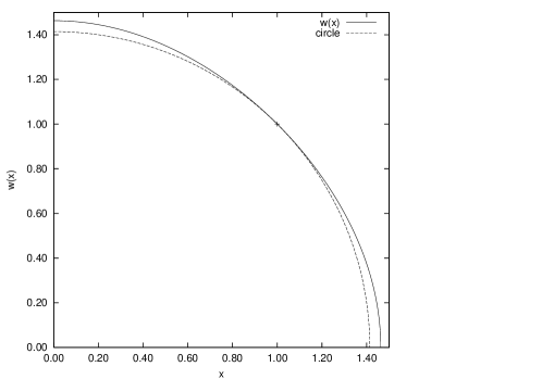
Figure 3: Plot from Bender et al. [BenderBeDeFe02] of a quarter of the optimal limiting boundary curve for the unconstrained problem; the dotted line is a circle.

In reconfigurable computing on field-programmable gate arrays (FPGAs), varying processor sizes give rise to a generalization of our problem: place a set of rectangular modules on a grid to minimize the overall weighted sum of $L_{1}$ distances between modules. Ahmadinia et al. [abftv-orcdprd-04] give an optimal $\Theta(n\log n)$ algorithm for finding an optimal feasible location for a module given a set of $n$ existing modules. At this point, no results are known for the general off-line problem (place $n$ modules simultaneously) or for on-line versions.

Another related problem is min-sum $k$-clustering: separate a graph into $k$ clusters to minimize the sum of distances between nodes in the same cluster. For general graphs, Sahni and Gonzalez [sahni76] show it is NP-hard to approximate this problem to within any constant factor for $k\geq 3$. In a metric space, Guttmann-Beck and Hassin [guttmannbeck98] give a $2$-approximation, Indyk [indyk99a] gives a PTAS for $k=2$, and Bartel et al. [bartal01] give an $O((1/\epsilon)\log^{1+\epsilon}n)$-approximation for general $k$.

Fekete and Meijer [fm-mdgmwc-04] consider the problem of maximizing the average $L_{1}$ distance. They give a PTAS for this dispersion problem in $\Re^{d}$ for constant $d$, and show that an optimal set of any fixed size can be found in $O(n)$ time.

Our Results.

We consider algorithms for minimizing the average $L_{1}$ distance between allocated processors in a mesh supercomputer. In particular, we give the following results:

• We prove that a greedy algorithm we call MM is a $\frac{7}{4}$-approximation algorithm for $2D$ grids. This reduces the previous best factor of 2 [krumke97]. We show that this analysis is tight.

• We present a simple generalization of MM to $d$-dimensional grids and prove that it gives a $2-\frac{1}{2d}$ approximation, which is tight.

• We give a polynomial-time approximation scheme (PTAS) for points in $\Re^{d}$ for constant $d$.

• Using simulations, we compare the allocation performance of MM to that of other algorithms. As a byproduct, we get insight on how to place a stream of jobs in an online setting.

• We give an algorithm to exactly solve the 2-dimensional case for $k=3$ in time $O(n\log n)$.

• We prove that the $d$-dimensional version of MC1x1 has approximation factor at most $d$ times that of MM.

Our work also led to a linear-time dynamic programming algorithm for the 1-dimensional problem of points on a line or ring; see Leung et al. [benderBDFL03] for details.

2 Algorithms for Two-Dimensional Point Sets

2.1 Manhattan Median Algorithm

Given a set $S$ of $k$ points in the plane, a point that minimizes the total $L_{1}$ distance to these points is called an ($L_{1}$) median. Given the nature of $L_{1}$ distances, this is a point whose $x$-coordinate (resp. $y$-coordinate) is the median of the $x$ (resp. $y$) values of the given point set. We can always pick a median whose coordinates are from the coordinates in $S$. There is a unique median if $k$ is odd; if $k$ is even, possible median coordinates may form intervals.

The natural greedy algorithm for our clustering problem is as follows:

Consider the set $I$ containing the $O(n^{2})$ intersection points of the horizontal and vertical lines through the points of input P. For each point $p\in I$ do: 1. Take the $k$ points closest to $p$ (using the $L_{1}$ metric), breaking ties arbitrarily. 2. Compute the total pairwise distance between all $k$ points. Return the set of $k$ points with smallest total pairwise distance.

We call this strategy MM, for Manhattan Median. We prove that MM is a $\frac{7}{4}$-approximation on 2D meshes. (Note that Krumke et al. [krumke97] call a minor variation of this algorithm Gen-Alg and show it is a 2-approximation in arbitrary metric spaces.)

For $S\subseteq P$, let $|S|$ denote the sum of $L_{1}$ distances between points in $S$. For a point $p$ in the plane, we use $p_{x}$ and $p_{y}$ to denote its $x$- and $y$-coordinates respectively.

Lemma 1

MM is not better than a $7/4$ approximation.

Proof

For a class of examples establishing the lower bound, consider the situation shown in Figure 4. For any $\epsilon>0$, it has clusters of $k/2$ points at $(0,0)$ and $(1,0)$. In addition, it has clusters of $k/8$ points at $(0,\pm(1-\epsilon))$, $(1,\pm(1-\epsilon))$, $(2-\epsilon,0)$, and $(-1+\epsilon,0)$. The best choices of median are $(0,0)$ and $(1,0)$, which yield a total distance of $7k^{2}(1-\Theta(\epsilon))/16$. The optimal solution is the points at $(0,0)$ and $(1,0)$, which yield a total distance of $k^{2}/4$. ∎

Figure 4: A class of examples where MM yields a ratio of $7/4$.

Now we show that $7/4$ is indeed the worst-case bound. We focus on possible worst-case arrangements and use local optimality to restrict the possible arrangements until the claim follows.

Let OPT be a subset of $P$ of size $k$ for which $|\mbox{\it OPT}|$ is minimum. Without loss of generality assume that the origin is a median point of OPT. This means that at most $k/2$ points of OPT have positive $x$-coordinates (similarly negative $x$-coordinates, positive $y$-coordinates, and negative $y$-coordinates). Let MM be the set of $k$ points closest to the origin. Since this is one candidate solution for the algorithm, its sum of pairwise distances is at least as high as that of the solution returned by the algorithm.

Without loss of generality, assume that the largest $L_{1}$ distance of a point in MM to the origin is 1, so MM lies in the $L_{1}$ unit circle $C$. (Note that $C$ is diamond-shaped.) We say that points are either inside $C$, on $C$, or outside $C$. All points of $P$ inside $C$ are in MM and at least some points on $C$ are in MM. If there are more than $k$ points on and inside $C$, we select all points inside $C$ plus those points on $C$ maximizing $|\mbox{\it MM}|$.

Clearly $1\leq|\mbox{\it MM}|/|\mbox{\it OPT}|$. Let $\rho_{k}$ be the supremum of $|\mbox{\it MM}|/|\mbox{\it OPT}|$ over all inputs $P$. By assuming that ties are broken badly, we can assume that there is an input for which $|\mbox{\it MM}|/|\mbox{\it OPT}|=\rho_{k}$:

Lemma 2

For any $n$ and $k$, there are point sets $P$ with $|P|=n$ for which $|\mbox{\it MM}|/|\mbox{\it OPT}|$ attains the value $\rho_{k}$.

Proof

The set of arrangements of $n$ points in the unit circle $C$ is a compact set in $2d$-dimensional space. By our assumption on breaking ties, $|\mbox{\it MM}|/|\mbox{\it OPT}|$ is upper semicontinuous, so it attains a maximum.∎

We show that $|\mbox{\it MM}|$ is at most $7/4$ times larger than $|\mbox{\it OPT}|$.

Theorem 2.1

MM is a $7/4$-approximation algorithm for minimizing the sum of pairwise $L_{1}$ distances in a 2D mesh.

Proof

For ease of presentation, we assume without loss of generality that $P=\mbox{\it MM}\cup\mbox{\it OPT}$. Let $B=\mbox{\it OPT}\cap\mbox{\it MM}$, $O=\mbox{\it OPT}-B$ and $A=\mbox{\it MM}-B$.

Claim 0: No point $p\in O$ lies outside $C$.

If a point $p\in O$ lies outside $C$ we can move it a little closer to the origin without entering $C$. Since it remains outside $C$, the point does not become part of MM, so $|\mbox{\it OPT}|$ is reduced, $|\mbox{\it MM}|$ remains the same and the ratio $|\mbox{\it MM}|/|\mbox{\it OPT}|$ increases, which is impossible.

Claim 1: All points inside $C$ are in MM.

It follows from the definition of MM that all points inside $C$ are in MM. Notice that this implies that no point $p\in O$ can lie inside $C$.

Claim 2: Without loss of generality, we may assume that the origin is also a median of MM.

Suppose that the origin is not a median of MM. We consider the case when more than $k/2$ points of MM have positive $y$-coordinate; the other cases are handled analogously. We set the $y$-coordinate of the point in MM with smallest positive $y$-coordinate to zero. By assumption, this causes the point to move away from at least as many points of MM as it moves toward. Thus, $|\mbox{\it MM}|$ does not decrease. The origin is a median of OPT so $|\mbox{\it OPT}|$ does not increase. Therefore, the ratio $|\mbox{\it MM}|/|\mbox{\it OPT}|$ cannot decrease. Since the ratio cannot increase by assumption, it must remain the same. Thus, we have constructed a point set achieving $|\mbox{\it MM}|/|\mbox{\it OPT}|=\rho_{k}$ with one fewer point having positive $y$-coordinate. Repeating this process will make some point on the line $y=0$ a median.

Claim 3: No point $p\in A$ lies inside $C$.

Suppose there is a $p\in A$ that lies inside $C$. Moving $p$ away from the origin increases MM because $p$ is moved further away from the median of MM. Since $p\notin\mbox{\it OPT}$, OPT does not increase, although it may decrease. So $|\mbox{\it MM}|/|\mbox{\it OPT}|$ increases, which is impossible. This implies that all points inside $C$ are in $B$ and that points from $A$ and $O$ lie on the boundary of $C$.

Claim 4: Without loss of generality, we may assume that all points $p\in A$ on $C$ lie in a corner of $C$.

Suppose $p\in A$ lies on an edge of $C$ but not in a corner. Let $D$ be the sum of the $L_{1}$ distances from $p$ to all points in $\mbox{\it MM}-{p}$. Consider the set $Q$ of all points $q$ for which the sum of the $L_{1}$ distances from $q$ to all points in $\mbox{\it MM}-{p}$ is at most $D$. The sum of distances is the sum of convex functions so it is also a convex function and the set $Q$ is a convex polygon through $p$. Therefore, we can move $p$ along the edge of $C$ on which it lies so that it either moves outside of $Q$ or remains on the boundary of $Q$. In former case, $|\mbox{\it MM}|$ increases. In the latter, $|\mbox{\it MM}|$ remains the same. In either case, $|\mbox{\it OPT}|$ stays the same or decreases. If $|\mbox{\it MM}|$ increases and/or $|\mbox{\it OPT}|$ decreases, $|\mbox{\it MM}|/|\mbox{\it OPT}|$ increases which is impossible. If both stay the same, we can move $p$ until it reaches a corner of $C$. For an illustration of what the configuration may look like see Figure 5(a).

Figure 5: Points of $A$, $O$ and $B$ (a) after claim 4 and (b) during motion used in claim 5.

Claim 5: Without loss of generality we may assume that all points in $O\cup B$ lie in a corner of $C$ or on the origin.

We prove the claim by contradiction. Suppose there is a set of points $S$ for which the claim is false. Let $p\in O\cup B$ be a point that does not lie in a corner of $C$ or on the origin. Let $S(p)$ be the points that lie on the axis-parallel rectangle through $p$ with corners on $C$. The set $S(p)$ is illustrated in Figure 5(b). We move the points in $S(p)$ simultaneously in such a way that they stay on an axis-parallel rectangle with corners on $C$. For example we move all points in $S(p)$ with maximal $y$-coordinates but not on $C$ upwards by $\epsilon$. We move all points in $S(p)$ with maximal $y$-coordinates and on $C$ upwards while remaining on $C$. Similarly the other points of $S(p)$ move either left, right or down. We choose $\epsilon$ small enough such that no point from $S\setminus S(p)$ enters the rectangle on which $S(p)$ lies. This move changes $|\mbox{\it MM}|$ by some amount $\delta_{a}$ and $|\mbox{\it OPT}|$ by some amount $\delta_{o}$. However if we move all points in the opposite direction (i.e. points with maximal $y$-coordinates downwards, etc.) $|\mbox{\it MM}|$ and $|\mbox{\it OPT}|$ change by $-\delta_{a}$ and $-\delta_{o}$ respectively. So if $\delta_{a}/\delta_{o}\neq\rho_{k}$, one of these two moves increases $|\mbox{\it MM}|/|\mbox{\it OPT}|$, which is impossible. If $\delta_{a}/\delta_{o}=\rho_{k}$ we keep moving the points in the same direction until there is a combinatorial change, i.e. a point from $S\setminus S(p)$ enters the rectangle on which $S(p)$ lies, a point in $S(p)$ reaches $C$, or the rectangle collapses into a line. Each combinatorial change decreases the number of rectangles on which the points lie, increases the number of points on $C$, or moves points to one of the coordinate axes. Since none of these changes is ever undone, we can then repeat this argument until all points of $S$ lie on a corner of $C$ or on the origin.

We can now complete the proof of Theorem 2.1. Let $b$ denote the number of points at the origin. These points are all in $B=\mbox{\it OPT}\cap\mbox{\it MM}$ since they were originally inside $C$. Let $a_{0},a_{1},a_{2},a_{3}$ and $o_{0},o_{1},o_{2},o_{3}$ be the points of MM and OPT at the north, east, south and west corners of $C$ respectively. The value of $|\mbox{\it MM}|$ is $2\sum_{0\leq i<j\leq 3}a_{i}a_{j}+\sum_{0\leq i\leq 3}ba_{i}~{}~{}=~{}~{}2\sum_{0\leq i<j\leq 3}a_{i}a_{j}+b(k-b)$ which is maximal when each value $a_{i}$ is equal to $\lceil(k-b)/4\rceil$ or $\lfloor(k-b)/4\rfloor$. The value of $|\mbox{\it OPT}|$ is $2\sum_{0\leq i<j\leq 3}o_{i}o_{j}+b(k-b)$ which is minimal when $o_{0}=k-b$ and $o_{1}=o_{2}=o_{3}=0$. The origin must be a median of OPT since none of our transformations move a point between quadrants. Thus, if $b<k/2$, the minimum value for $|\mbox{\it OPT}|$ occurs when $o_{0}=k/2$ and $o_{1}=k/2-b$. So if $b<k/2$ we have $\frac{|\mbox{\it MM}|}{|\mbox{\it OPT}|}\leq\frac{\frac{12(k-b)^{2}}{16}+b(k-b)}{k(\frac{k}{2}-b)+b(k-b)}$ from which it follows that $\frac{|\mbox{\it MM}|}{|\mbox{\it OPT}|}\leq\frac{3k^{2}-2kb-b^{2}}{2k^{2}-4b^{2}}.$ This is a convex function of $b$ in the interval $0\leq b<k/2$ whose values are smaller than 7/4.

If $b\geq k/2$ we have $\frac{|\mbox{\it MM}|}{|\mbox{\it OPT}|}\leq\frac{\frac{12(k-b)^{2}}{16}+b(k-b)}{b(k-b)}~{}=~{}\frac{3k+b}{4b}$ which is maximal when $b=k/2$ in which case $|\mbox{\it MM}|/|\mbox{\it OPT}|=7/4$. Notice that $n$ has to be at least $11k/8$ for this value to be obtained since we need $a_{i}=k/8$ for all $i$ and $o_{0}=k/2$ where MM and OPT can share the points in the north corner of $C$. For smaller values of $n$ we can add extra points to the corners of $C$ until $n=11k/8$, so MM increases and OPT decreases. Since $|\mbox{\it MM}/|\mbox{\it OPT}|=7/4$ when $n=11k/8$ we have $|\mbox{\it MM}/|\mbox{\it OPT}|\leq 7/4$ for all values of $k$. Therefore the theorem holds. ∎

2.2 Analysis of MC1x1

MC was originally presented as a heuristic algorithm, but we prove that MC1x1 has approximation ratio $(2-2/k)d$ in dimension $d$. Krumke et al. [krumke97] used the same ideas to prove that a variant of MM is a $(2-2/k)$-approximation algorithm; their argument also applies to MM.

Theorem 2.2

MC1x1 is a $(2-2/k)d$-approximation algorithm for minimizing the sum of pairwise $L_{1}$ distances in a $d$-dimensional mesh.

Proof

Recall that MC1x1 minimizes the sum of the selected points’ shell numbers. Let point $v$ be the center of the shells for the selected allocation and let $\sigma$ be the sum of the shell numbers for points of MC1x1. First, we bound $|\mbox{\it MC1x1}|$ in terms of $\sigma$. The total distance from $v$ to each point of MC1x1 is at most $\sigma d$ since a point in shell $i$ is at most $id$ steps from $v$. Thus, $|\mbox{\it MC1x1}|\leq(k-1)\sigma d$ since this is the distance if all paths are routed through $v$.

Now we bound $|\mbox{\it OPT}|$ in terms of $\sigma$. For this, we use the concept of a star, which is a set of points with one identified as its center. The length of a star is the total distance between the center and its other points. The smallest star with $k$ points has length at least $\sigma$ since a point distance $i$ from the star’s center is in the $i^{\text{th}}$ shell around that center. Thus, the total distance from one point of OPT to the others is at least $\sigma$. Since summing the lengths of stars of OPT with each point as the center counts the distance between each pair of points twice, $|\mbox{\it OPT}|\geq k\sigma/2$ and the lemma follows by combining our bounds. ∎

2.3 Fast Algorithm for $k=3$

Theorem 2.3

Let $P$ be a set of $n$ points in the plane. The subset of $P$ of size 3 with minimum total pairwise $L_{1}$ distance can be found in $O(n\log n)$ time.

Proof

Let $S=\{s_{0},s_{1},s_{2}\}$ be a subset of $P$. Label the $x$- and $y$-coordinates of a point $s\in S$ with $(x_{a},y_{b})$ with $0\leq a<3$ and $0\leq b<3$ so that $x_{0}\leq x_{1}\leq x_{2}$ and $y_{0}\leq y_{1}\leq y_{2}$. The total pairwise $L_{1}$ distance of $S$ is $2(x_{2}-x_{0})+2(y_{2}-y_{0})$. Consider the smallest Steiner star of $S$, which has center $(x_{1},y_{1})$. Its length is $(x_{2}-x_{0})+(y_{2}-y_{0})$. Since the total pairwise distance and length of the smallest Steiner star are constant multiples of each other, the subset of size 3 having minimum total pairwise distance also has the smallest Steiner star.

Let $c$ be the center of the smallest Steiner star of 3 points of $P$. By the discussion above, the three points having this Steiner star also have minimum total pairwise distance. These points are the three closest points to $c$ or there would have been a smaller Steiner star. Therefore, these points correspond to a cell on the order-3 Voronoi diagram of $P$. Since this diagram can be found in $O(n\log n)$ time [l-knnvd-82], the theorem follows. ∎

3 PTAS for Two Dimensions

Let $w(S,T)$ be the sum of all the distances from points in $S$ to points in $T$. Let $w_{x}(S,T)$ and $w_{y}(S,T)$ be the sum of $x$- and $y$- distances from points in $S$ to points in $T$, respectively. So $w(S,T)=w_{x}(S,T)+w_{y}(S,T)$. Let $w(S)=w(S,S)$, $w_{x}(S)=w_{x}(S,S)$, and $w_{y}(S)=w_{y}(S,S)$. We call $w(S)$ the weight of $S$.

Let $S=\{s_{0},s_{1},\ldots,s_{k-1}\}$ be a minimum-weight subset of $P$, where $k$ is an integer greater than 1. We label the $x$- and $y$-coordinates of a point $s\in S$ by some $(x_{a},y_{b})$ with $0\leq a<k$ and $0\leq b<k$ such that $x_{0}\leq x_{1}\leq\ldots\leq x_{k-1}$ and $y_{0}\leq y_{1}\leq\ldots\leq y_{k-1}$. (Note that in general, $a\neq b$ for a point $s=(x_{a},y_{b})$.) We can derive the following equations: $w_{x}(S)~{}=~{}(k-1)(x_{k-1}-x_{0})+(k-3)(x_{k-2}-x_{1})+~{}\ldots~{}$ and $w_{y}(S)~{}=~{}(k-1)(y_{k-1}-y_{0})+(k-3)(y_{k-2}-y_{1})+~{}\ldots~{}$ We show that there is a polynomial-time approximation scheme (PTAS), i.e., for any fixed positive $m=1/\varepsilon$, there is a polynomial approximation algorithm that finds a solution within $(1+\varepsilon)$ of the optimum.

The basic idea is similar to the one used by Fekete and Meijer [fm-mdgmwc-04] to select a set of points maximizing the overall distance: We find (by enumeration) a subdivision of an optimal solution into $m\times m$ rectangular cells $C_{ij}$, each containing a specific number $k_{ij}$ of selected points. The points from each cell $C_{ij}$ are selected in a way that minimizes the total distance to all other cells except for the $m-1$ cells in the same “horizontal” strip or the $m-1$ cells in the same “vertical” strip. As it turns out, this can be done in a way that the total neglected distance within the strips is bounded by a small fraction of the weight of an optimal solution, yielding the desired approximation property. See Figure 6 for the setup.

Figure 6: Dividing the point set into horizontal and vertical strips.

For ease of presentation, we assume that $k$ is a multiple of $m$ and $m>2$. Approximation algorithms for other values of $k$ can be constructed in a similar fashion. Consider a division of the plane by a set of $m+1$ $x$-coordinates $\xi_{0}\leq\xi_{1}\leq\ldots\leq\xi_{m}$. Let $X_{i}:=\{p=(x,y)\mid\xi_{i}\leq x\leq\xi_{i+1}\}$ be the vertical strip between coordinates $\xi_{i}$ and $\xi_{i+1}$. By enumeration of possible values of $\xi_{0},\ldots,\xi_{m}$ we may assume that each of the $m$ strips $X_{i}$ contains precisely $k/m$ points of an optimal solution. (A small perturbation does not change optimality or approximation properties of solutions. Thus, without loss of generality, we assume that no pair of points share either $x$-coordinate or $y$-coordinate.)

In a similar manner, assume we know $m+1$ $y$-coordinates $\eta_{0}\leq\eta_{1}\leq\ldots\leq\eta_{m}$ so that an optimal solution has precisely $k/m$ points in each horizontal strip $Y_{i}:=\{p=(x,y)\mid\eta_{i}\leq y\leq\eta_{i+1}\}$.

Let $C_{ij}:=X_{i}\cap Y_{j}$, and let $k_{ij}$ be the number of points in OPT that are chosen from $C_{ij}$. Since for all $i,j\in\{1,2,\ldots,m\}$,

$$\sum_{0\leq l<m}k_{lj}=\sum_{0\leq l<m}k_{il}=k/m,$$

we may assume by enumeration over the $O(k^{m})$ possible partitions of $k/m$ into $m$ pieces that we know all the numbers $k_{ij}$.

Finally, define the vector $\nabla_{ij}:=((2i+1-m)k/m,(2j+1-m)k/m)$. Our approximation algorithm is as follows: from each cell $C_{ij}$, choose $k_{ij}$ points that are minimum in direction $\nabla_{ij}$, i.e., select points $p=(x,y)$ for which $(x(2i+1-m)k/m,y(2j+1-m)k/m)$ is minimum. For an illustration, see Figure 7.

It can be shown that selecting points of $C_{ij}$ this way minimizes the sum of $x$-distances to points not in $X_{i}$ and the sum of $y$-distances to points not in $Y_{j}$. Technical details are described in the following. We summarize:

Theorem 3.1

The problem of selecting a subset of minimum total $L_{1}$ distance for a set of points in $\Re^{2}$ allows a PTAS.

Figure 7: Selecting points in cell $C_{12}$.

Correctness of the PTAS

Let MM be the point set selected by the algorithm described in Section 3. It is clear that MM can be computed in polynomial time. We will proceed by a series of lemmas to determine how well $w(\mbox{\it MM})$ approximates $w(\mbox{\it OPT})$. In the following, we consider the distances involving points from a particular cell $C_{ij}$. Let $\mbox{\it MM}_{ij}$ be the set of $k_{ij}$ points that are selected from $C_{ij}$ by the heuristic, and let $\mbox{\it OPT}_{ij}$ be a set of $k_{ij}$ points of an optimal solution that are attributed to $C_{ij}$. Let $\mbox{\it MM}_{i\bullet}$, $\mbox{\it OPT}_{i\bullet}$, $\mbox{\it MM}_{\bullet j}$ and $\mbox{\it OPT}_{\bullet j}$ be the set of $k/m$ points selected from $X_{i}$ and $Y_{j}$ by the heuristic and an optimal algorithm respectively. Finally $\overline{\mbox{\it MM}}_{i\bullet}:=\mbox{\it MM}\setminus\mbox{\it MM}_{i\bullet}$, $\overline{\mbox{\it MM}}_{\bullet j}:=\mbox{\it MM}\setminus\mbox{\it MM}_{\bullet j}$, $\overline{\mbox{\it OPT}}_{i\bullet}:=\mbox{\it OPT}\setminus\mbox{\it OPT}_{i\bullet}$ and $\overline{\mbox{\it OPT}}_{\bullet j}:=\mbox{\it OPT}\setminus\mbox{\it OPT}_{\bullet j}$.

For the rest of the notation notice that

$$w(HEU) = \sum_{i,j}{[w_{x}(\mbox{\it MM}_{ij},\overline{\mbox{\it MM}}_{i\bullet})+w_{y}(\mbox{\it MM}_{ij},\overline{\mbox{\it MM}}_{\bullet j})]}$$

$$+ \sum_{i}{w_{x}(\mbox{\it MM}_{i\bullet})}+\sum_{j}{w_{y}(\mbox{\it MM}_{\bullet j})}.$$

We first show that the first part is smaller that $w(\mbox{\it OPT})$. We then show that the second and third part are small fractions of $w(HEU)$.

Lemma 3

$$w_{x}(\mbox{\it MM}_{ij},\overline{\mbox{\it MM}}_{i\bullet})+w_{y}(\mbox{\it MM}_{ij},\overline{\mbox{\it MM}}_{\bullet j})$$

$$\leq w_{x}(\mbox{\it OPT}_{ij},\overline{\mbox{\it OPT}}_{i\bullet})+w_{y}(\mbox{\it OPT}_{ij},\overline{\mbox{\it OPT}}_{\bullet j}).$$

Proof

Consider a point $p\in\mbox{\it OPT}_{ij}\setminus\mbox{\it MM}_{ij}$. We will replace it with an arbitrary point $p^{\prime}\in\mbox{\it MM}_{ij}\setminus\mbox{\it OPT}_{ij}$ that was chosen by the heuristic instead of $p$. Let $p-p^{\prime}=h=(h_{x},h_{y})$. When replacing $p^{\prime}$ in MM by $p$, we increase the $x$-distance to the $ik/m$ points left of $C_{ij}$ by $h_{x}$, while decreasing the $x$-distance to $(m-i-1)k/m$ points right of $C_{ij}$ by $h_{x}$. In the balance, this yields a change of $((2i+1-m)k/m)h_{x}$. Similarly, we get a change of $((2j+1-m)k/m)h_{y}$ for the $y$-coordinates. Since $p^{\prime}$ was chosen to minimize the inner product $\langle p^{\prime},\nabla_{ij}\rangle$ we know that the inner product $\langle h,\nabla_{ij}\rangle\geq 0$, so the overall change of distances is positive.

Performing these replacements for all points in $\mbox{\it MM}\setminus\mbox{\it OPT}$, we can transform MM to OPT, while increasing the sum of distances $w_{x}(\mbox{\it MM}_{ij},\overline{\mbox{\it MM}}_{i\bullet})+w_{y}(\mbox{\it MM}_{ij},\overline{\mbox{\it MM}}_{\bullet j})$ to the sum $w_{x}(\mbox{\it OPT}_{ij},\overline{\mbox{\it OPT}}_{i\bullet})+w_{y}(\mbox{\it OPT}_{ij},\overline{\mbox{\it OPT}}_{\bullet j})$.∎

Corollary 1

$$\sum_{i,j}{w_{x}(\mbox{\it MM}_{ij},\overline{\mbox{\it MM}}_{i\bullet})+w_{y}(\mbox{\it MM}_{ij},\overline{\mbox{\it MM}}_{\bullet j})}\leq w(\mbox{\it OPT}).$$

In the following two lemmas we show that

$$\sum_{i}w_{x}(\mbox{\it MM}_{i\bullet})$$

is a small fraction of $w(\mbox{\it MM})$. Analogous proofs can be given for

$$\sum_{j}w_{y}(\mbox{\it MM}_{\bullet j}).$$

Lemma 4

$$\sum_{0<i<m-1}w_{x}(\mbox{\it MM}_{i\bullet})~{}\leq~{}\frac{w_{x}(\mbox{\it MM})}{m-2}.$$