Reduced cost-based ranking for generating promising subproblems

Abstract

In this paper, we propose an effective search procedure that interleaves two steps: subproblem generation and subproblem solution. We mainly focus on the first part. It consists of a variable domain value ranking based on reduced costs. Exploiting the ranking, we generate, in a Limited Discrepancy Search tree, the most promising subproblems first. An interesting result is that reduced costs provide a very precise ranking that allows to almost always find the optimal solution in the first generated subproblem, even if its dimension is significantly smaller than that of the original problem. Concerning the proof of optimality, we exploit a way to increase the lower bound for subproblems at higher discrepancies. We show experimental results on the TSP and its time constrained variant to show the effectiveness of the proposed approach, but the technique could be generalized for other problems.

1 Introduction

In recent years, combinatorial optimization problems have been tackled with hybrid methods and/or hybrid solvers [11, 18, 13, 19]. The use of problem relaxations, decomposition, cutting planes generation techniques in a Constraint Programming (CP) framework are only some examples. Many hybrid approaches are based on the use of a relaxation $R$, i.e. an easier problem derived from the original one by removing (or relaxing) some constraints. Solving $R$ to optimality provides a bound on the original problem. Moreover, when the relaxation is a linear problem, we can derive reduced costs through dual variables often with no additional computational cost. Reduced costs provide an optimistic esteem (a bound) of each variable-value assignment cost. These results have been successfully used for pruning the search space and for guiding the search toward promising regions (see [9]) in many applications like TSP [12], TSPTW [10], scheduling with sequence dependent setup times [8] and multimedia applications [4].

We propose here a solution method, depicted in Figure 1, based on a two step search procedure that interleaves ($i$) subproblem generation and ($ii$) subproblem solution. In detail, we solve a relaxation of the problem at the root node and we use reduced costs to rank domain values; then we partition the domain of each variable $X_{i}$ in two sets, i.e., the good part $D_{i}^{good}$ and the bad part $D_{i}^{bad}$. We search the tree generated by using a strategy imposing on the left branch the branching constraint $X_{i}\in D_{i}^{good}$ while on the right branch we impose $X_{i}\in D_{i}^{bad}$. At each leaf of the subproblem generation tree, we have a subproblem which can now be solved (in the subproblem solution tree).

Exploring with a Limited Discrepancy Strategy the resulting search space, we obtain that the first generated subproblems are supposed to be the most promising and are likely to contain the optimal solution. In fact, if the ranking criterion is effective (as the experimental results will show), the first generated subproblem (discrepancy equal to 0) $P^{(0)}$, where all variables range on the good domain part, is likely to contain the optimal solution. The following generated subproblems (discrepancy equal to 1) $P^{(1)}_{i}$ have all variables but the $i$-th ranging on the good domain and are likely to contain worse solutions with respect to $P^{(0)}$, but still good. Clearly, subproblems at higher discrepancies are supposed to contain the worst solutions.

A surprising aspect of this method is that even by using low cardinality good sets, we almost always find the optimal solution in the first generated subproblem. Thus, reduced costs provide extremely useful information indicating for each variable which values are the most promising. Moreover, this property of reduced costs is independent of the tightness of the relaxation. Tight relaxations are essential for the proof of optimality, but not for the quality of reduced costs. Solving only the first subproblem, we obtain a very effective incomplete method that finds the optimal solution in almost all test instances.

To be complete, the method should solve all subproblems for all discrepancies to prove optimality. Clearly, even if each subproblem could be efficiently solved, if all of them should be considered, the proposed approach would not be applicable. The idea is that by generating the optimal solution soon and tightening the lower bound with considerations based on the discrepancies shown in the paper, we do not have to explore all subproblems, but we can prune many of them.

In this paper, we have considered as an example the Travelling Salesman Problem and its time constrained variant, but the technique could be applied to a large family of problems.

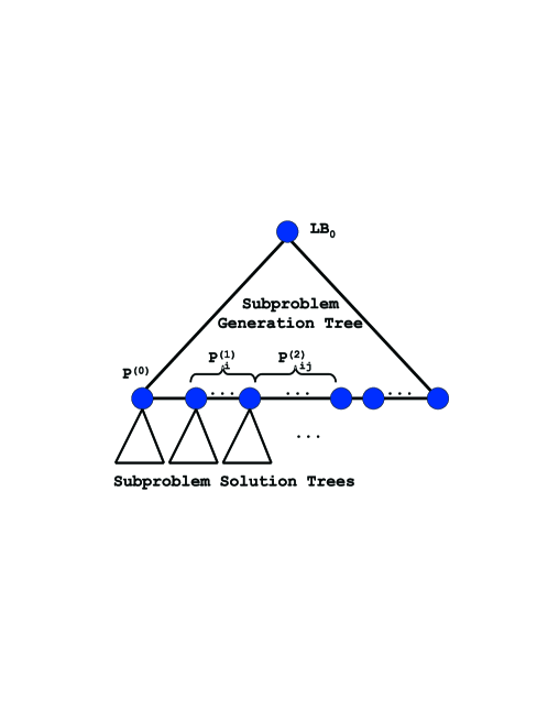
Figure 1: The structure of the search tree.

The contribution of this paper is twofold: ($i$) we show that reduced costs provide an extremely precise indication for generating promising subproblems, and ($ii$) we show that LDS can be used to effectively order the subproblems. In addition, the use of discrepancies enables to tighten the problem bounds for each subproblem.

The paper is organized as follows: in Section 2 we give preliminaries on Limited Discrepancy Search (LDS), on the TSP and its time constrained variant. In Section 3 we describe the proposed method in detail. Section 4 discusses the implementation, focussing mainly on the generation of the subproblems using LDS. The quality of the reduced cost-based ranking is considered in Section 5. In this section also the size of subproblems is tuned. Section 6 presents the computational results. Conclusion and future work follow.

2 Preliminaries

2.1 Limited Discrepancy Search

Limited Discrepancy Search (LDS) was first introduced by Harvey and Ginsberg [15]. The idea is that one can often find the optimal solution by exploring only a small fraction of the space by relying on tuned (often problem dependent) heuristics. However, a perfect heuristic is not always available. LDS addresses the problem of what to do when the heuristic fails.

Thus, at each node of the search tree, the heuristic is supposed to provide the good choice (corresponding to the leftmost branch) among possible alternative branches. Any other choice would be bad and is called a discrepancy. In LDS, one tries to find first the solution with as few discrepancies as possible. In fact, a perfect heuristic would provide us the optimal solution immediately. Since this is not often the case, we have to increase the number of discrepancies so as to make it possible to find the optimal solution after correcting the mistakes made by the heuristic. However, the goal is to use only few discrepancies since in general good solutions are provided soon.

LDS builds a search tree in the following way: the first solution explored is that suggested by the heuristic. Then solutions that follow the heuristic for every variable but one are explored: these solutions are that of discrepancy equal to one. Then, solutions at discrepancy equal to two are explored and so on.

It has been shown that this search strategy achieves a significant cutoff of the total number of nodes with respect to a depth first search with chronological backtracking and iterative sampling [20].

2.2 TSP and TSPTW

Let $G=(V,A)$ be a digraph, where $V=\{1,\dots,n\}$ is the vertex set and $A=\{(i,j):i,j\in V\}$ the arc set, and let $c_{ij}\geq 0$ be the cost associated with arc $(i,j)\in A$ (with $c_{ii}=+\infty$ for each $i\in V$). A Hamiltonian Circuit (tour) of $G$ is a partial digraph $\bar{G}=(V,\bar{A})$ of $G$ such that: $|\bar{A}|=n$ and for each pair of distinct vertices $v_{1},v_{2}\in V$, both paths from $v_{1}$ to $v_{2}$ and from $v_{2}$ to $v_{1}$ exist in $\bar{G}$ (i.e. digraph $\bar{G}$ is strongly connected).

The Travelling Salesman Problem (TSP) looks for a Hamiltonian circuit $G^{*}=(V,A^{*})$ whose cost $\sum_{(i,j)\in A^{*}}c_{ij}$ is a minimum.

A classic Integer Linear Programming formulation for TSP is as follows:

$$v(TSP) =\min\sum_{i\in V}\sum_{j\in V}c_{ij}\,x_{ij}$$ (1)

subject to $$\sum_{i\in V}x_{ij}=1,\qquad j\in V$$ (2)

$$\sum_{j\in V}x_{ij}=1,\qquad i\in V$$ (5)

$$\sum_{i\in S}\sum_{j\in V\setminus S}x_{ij}\geq 1,\qquad S\subset V,\;S\not=\emptyset$$

$$x_{ij}\hbox{~{}integer,~{}~{}}i,j\in V$$

where $x_{ij}=1$ if and only if arc $(i,j)$ is part of the solution. Constraints (2) and (5) impose in-degree and out-degree of each vertex equal to one, whereas constraints (5) impose strong connectivity.

Constraint Programming relies in general on a different model where we have a domain variable ${\rm\it Next}_{i}$ (resp. ${\rm\it Prev}_{i}$) that identifies cities visited after (resp. before) node $i$. Domain variable $Cost_{i}$ identifies the cost to be paid to go from node $i$ to node ${\rm\it Next}_{i}$.

Clearly, we need a mapping between the CP model and the ILP model: ${\rm\it Next}_{i}=j\;\Leftrightarrow\;x_{ij}=1$. The domain of variable ${\rm\it Next}_{i}$ will be denoted as $D_{i}$. Initially, $D_{i}=\{1,\dots,n\}$.

The Travelling Salesman Problem with Time Windows (TSPTW) is a time constrained variant of the TSP where the service at a node $i$ should begin within a time window $[a_{i},b_{i}]$ associated to the node. Early arrivals are allowed, in the sense that the vehicle can arrive before the time window lower bound. However, in this case the vehicle has to wait until the node is ready for the beginning of service.

As concerns the CP model for the TSPTW, we add to the TSP model a domain variable ${\rm\it Start}_{i}$ which identifies the time at which the service begins at node $i$.

A well known relaxation of the TSP and TSPTW obtained by eliminating from the TSP model constraints (5) and time windows constraints is the Linear Assignment Problem (AP) (see [3] for a survey). AP is the graph theory problem of finding a set of disjoint subtours such that all the vertices in $V$ are visited and the overall cost is a minimum. When the digraph is complete, as in our case, AP always has an optimal integer solution, and, if such solution is composed by a single tour, is then optimal for TSP satisfying constraints (5).

The information provided by the AP relaxation is a lower bound $LB$ for the original problem and the reduced cost matrix $\bar{c}$. At each node of the decision tree, each $\bar{c}_{ij}$ estimates the additional cost to pay to put arc $(i,j)$ in the solution. More formally, a valid lower bound for the problem where $x_{ij}=1$ is $LB|_{x_{ij}=1}=LB+\bar{c}_{ij}$. It is well-known that when the AP optimal solution is obtained through a primal-dual algorithm, as in our case (we use a C++ adaptation of the AP code described in [2]), the reduced cost values are obtained without extra computational effort during the AP solution. The solution of the AP relaxation at the root node requires in the worst case $O(n^{3})$, whereas each following AP solution can be efficiently computed in $O(n^{2})$ time through a single augmenting path step (see [2] for details). However, the AP does not provide a tight bound neither for the TSP nor for the TSPTW. Therefore we will improve the relaxation in Section 3.1.

3 The Proposed Method

In this section we describe the method proposed in this paper. It is based on two interleaved steps: subproblem generation and subproblem solution. The first step is based on the optimal solution of a (possibly tight) relaxation of the original problem. The relaxation provides a lower bound for the original problem and the reduced cost matrix. Reduced costs are used for ranking (the lower the better) variable domain values. Each domain is now partitioned according to this ranking in two sets called the good set and the bad set. The cardinality of the good set is problem dependent and is experimentally defined. However, it should be significantly lower than the dimension of the original domains.

Exploiting this ranking, the search proceeds by choosing at each node the branching constraint that imposes the variable to range on the good domain, while on backtracking we impose the variable to range on the bad domain. By exploring the resulting search tree by using an LDS strategy we generate first the most promising problems, i.e., those where no or few variables range on the bad sets.

Each time we generate a subproblem, the second step starts for optimally solving it. Experimental results will show that, surprisingly, even if the subproblems are small, the first generated subproblem almost always contains the optimal solution. The proof of optimality should then proceed by solving the remaining problems. Therefore, a tight initial lower bound is essential. Moreover, by using some considerations on discrepancies, we can increase the bound and prove optimality fast.

The idea of ranking domain values has been previously used in incomplete algorithms, like GRASP [5]. The idea is to produce for each variable the so called Restricted Candidate List (RCL), and explore the subproblem generated only by RCLs for each variable. This method provides in general a good starting point for performing local search. Our ranking method could in principle be applied to GRASP-like algorithms.

Another connection can be made with iterative broadening [14], where one can view the breadth cutoff as corresponding to the cardinality of our good sets. The first generated subproblem of both approaches is then the same. However, iterative broadening behaves differently on backtracking (it gradually restarts increasing the breadth cutoff).

3.1 Linear relaxation

In Section 2.2 we presented a relaxation, the Linear Assignment Problem (AP), for both the TSP and TSPTW. This relaxation is indeed not very tight and does not provide a good lower bound. We can improve it by adding cutting planes. Many different kinds of cutting planes for these problems have been proposed and the corresponding separation procedure has been defined [22]. In this paper, we used the Sub-tour Elimination Cuts (SECs) for the TSP. However, adding linear inequalities to the AP formulation changes the structure of the relaxation which is no longer an AP. On the other hand, we are interested in maintaining this structure since we have a polynomial and incremental algorithm that solves the problem. Therefore, as done in [10], we relax cuts in a Lagrangean way, thus maintaining an AP structure.

The resulting relaxation, we call it AP^cuts, still has an AP structure, but provides a tighter bound than the initial AP. More precisely, it provides the same objective function value as the linear relaxation where all cuts are added defining the sub-tour polytope. In many cases, in particular for TSPTW instances, the bound is extremely close to the optimal solution.

3.2 Domain partitioning

As described in Section 2.2, the solution of an Assignment Problem provides the reduced cost matrix with no additional computational cost. We recall that the reduced cost $\overline{c}_{ij}$ of a variable $x_{ij}$ corresponds to the additional cost to be paid if this variable is inserted in the solution, i.e., $x_{ij}=1$. Since these variables are mapped into CP variables Next, we obtain the same esteem also for variable domain values. Thus, it is likely that domain values that have a relative low reduced cost value will be part of an optimal solution to the TSP.

This property is used to partition the domain $D_{i}$ of a variable ${\rm\it Next}_{i}$ into $D_{i}^{good}$ and $D_{i}^{bad}$, such that $D_{i}=D_{i}^{good}\cup D_{i}^{bad}$ and $D_{i}^{good}\cap D_{i}^{bad}=\emptyset$ for all $i=1,\dots,n$. Given a ratio $r\geq 0$, we define for each variable ${\rm\it Next}_{i}$ the good set $D_{i}^{good}$ by selecting from the domain $D_{i}$ the values $j$ that have the $r*n$ lowest $\overline{c}_{ij}$. Consequently, $D_{i}^{bad}=D_{i}\setminus D_{i}^{good}$.

The ratio defines the size of the good domains, and will be discussed in Section 5. Note that the optimal ratio should be experimentally tuned, in order to obtain the optimal solution in the first subproblem, and it is strongly problem dependent. In particular, it depends on the structure of the problem we are solving. For instance, for the pure TSP instances considered in this paper, a good ratio is 0.05 or 0.075, while for TSPTW the best ratio observed is around 0.15. With this ratio, the optimal solution of the original problem is indeed located in the first generated subproblem in almost all test instances.

3.3 LDS for generating subproblems

In the previous section, we described how to partition variable domains in a good and a bad set by exploiting information on reduced costs. Now, we show how to explore a search tree on the basis of this domain partitioning. At each node corresponding to the choice of variable $X_{i}$, whose domain has been partitioned in $D_{i}^{good}$ and $D_{i}^{bad}$, we impose on the left branch the branching constraint $X_{i}\in D_{i}^{good}$, and on the right branch $X_{i}\in D_{i}^{bad}$. Exploring with a Limited Discrepancy Search strategy this tree, we first explore the subproblem suggested by the heuristic where all variable range on the good set; then subproblems where all variables but one range on the good set, and so on.

If the reduced cost-based ranking criterion is accurate, as the experimental results confirm, we are likely to find the optimal solution in the subproblem $P^{(0)}$ generated by imposing all variables ranging on the good set of values. If this heuristic fails once, we are likely to find the optimal solution in one of the $n$ subproblems ($P^{(1)}_{i}$ with $i\in\{1,\dots,n\}$) generated by imposing all variables but one (variable $i$) ranging on the good sets and one ranging on the bad set. Then, we go on generating $n(n-1)/2$ problems $P^{(2)}_{ij}$ all variables but two (namely $i$ and $j$) ranging on the good set and two ranging on the bad set are considered, and so on.

In Section 4 we will see an implementation of this search strategy that in a sense squeezes the subproblem generation tree shown in Figure 1 into a constraint.

3.4 Proof of optimality

If we are simply interested in a good solution, without proving optimality, we can stop our method after the solution of the first generated subproblem. In this case, the proposed approach is extremely effective since we almost always find the optimal solution in that subproblem.

Otherwise, if we are interested in a provably optimal solution, we have to prove optimality by solving all sub-problems at increasing discrepancies. Clearly, even if all subproblems could be efficiently solved, generating and solving all of them would not be practical. However, if we exploit a tight initial lower bound, as explained in Section 3.1, which is successively improved with considerations on the discrepancy, we can stop the generation of subproblems after few trials since we prove optimality fast.

An important part of the proof of optimality is the management of lower and upper bounds. The upper bound is decreased as we find better solutions, and the lower bound is increased as a consequence of discrepancy increase. The idea is to find an optimal solution in the first subproblem, providing the best possible upper bound.

The ideal case is that all subproblems but the first can be pruned since they have a lower bound higher than the current upper bound, in which case we only need to consider a single subproblem.

The initial lower bound ${\rm LB}_{0}$ provided by the Assignment Problem AP^cuts at the root node can be improved each time we switch to a higher discrepancy $k$. For $i\in\{1,\dots,n\}$, let $\overline{c}_{i}^{*}$ be the lowest reduced cost value associated with $D_{i}^{bad}$, corresponding to the solution of AP^cuts, i.e. $\overline{c}_{i}^{*}=\min_{j\in D_{i}^{bad}}{\overline{c}_{ij}}$. Clearly, a first trivial bound is ${\rm LB}_{0}+\min_{i\in\{1,\dots,n\}}\overline{c}_{i}^{*}$ for all problems at discrepancy greater than or equal to 1. We can increase this bound: let $L$ be the nondecreasing ordered list of $\overline{c}_{i}^{*}$ values, containing $n$ elements. $L[i]$ denotes the $i$-th element in $L$. The following theorem achieves a better bound improvement [21].

Theorem 3.1

For $k\in\{1,\dots,n\}$, ${\rm LB}_{0}+\sum_{i=1}^{k}L[i]$ is a valid lower bound for the subproblems corresponding to discrepancy k.

Proof

The proof is based on the concept of additive bounding procedures [6, 7] that states as follows: first we solve a relaxation of a problem $P$. We obtain a bound $LB$, in our case ${\rm LB}_{0}$ and a reduced-cost matrix $\overline{c}$. Now we define a second relaxation of $P$ having cost matrix $\overline{c}$. We obtain a second lower bound $LB^{(1)}$. The sum $LB+LB^{(1)}$ is a valid lower bound for $P$. In our case, the second relaxation is defined by the constraints imposing in-degree of each vertex less or equal to one plus a linear version of the k-discrepancy constraint: $\sum_{i\in V}\sum_{j\in D_{i}^{bad}}x_{ij}=k$. Thus, $\sum_{i=1}^{k}L[i]$ is exactly the optimal solution for this problem. $\Box$

Note that in general reduced costs are not additive, but in this case they are. As a consequence of this result, optimality is proven as soon as ${\rm LB}_{0}+\sum_{i=1}^{k}L[i]>{\rm UB}$ for some discrepancy $k$, where ${\rm UB}$ is the current upper bound. We used this bound in our implementation.

3.5 Solving each subproblem

Once the subproblems are generated, we can solve them with any complete technique. In this paper, we have used the method and the code described in [12] and in [10] for the TSPTW. As a search heuristic we have used the one behaving best for each problem.

4 Implementation

Finding a subproblem of discrepancy $k$ is equivalent to finding a set $S~{}\subseteq~{}\{1,\dots,n\}$ with $|S|=k$ such that

$$\begin{array}[]{ll}{\rm\it Next}_{i}\in D_{i}^{bad}&$for $i\in S$, and $\\ {\rm\it Next}_{i}\in D_{i}^{good}&$for $i\in\{1,\dots,n\}\setminus S.\end{array}$$

The search for such a set $S$ and the corresponding domain assignments have been ‘squeezed’ into a constraint, the discrepancy constraint discr_cst. It takes as input the discrepancy $k$, the variables ${\rm\it Next}_{i}$ and the domains $D_{i}^{good}$. Declaratively, the constraint holds if and only if exactly $k$ variables take their values in the bad sets.

Operationally, it keeps track of the number of variables that take their value in either the good or the bad domain. If during the search for a solution in the current subproblem the number of variables ranging on their bad domain is $k$, all other variables are forced to range on their good domain. Equivalently, if the number of variables ranging on their good domain is $n-k$, the other variables are forced to range on their bad domain.

The subproblem generation is defined as follows (in pseudo-code):

   for (k=0..n) {
     add(discr_cst(k,next,D_good));
     solve subproblem;
     remove(discr_cst(k,next,D_good));
   }

where k is the level of discrepancy, next is the array containing ${\rm\it Next}_{i}$, and D_good is the array containing $D_{i}^{good}$ for all $i\in\{1,\dots,n\}$. The command solve subproblem is shorthand for solving the subproblem which has been considered in Section 3.5.

A more traditional implementation of LDS (referred to as ‘standard’ in Table 1) exploits tree search, where at each node the domain of a variable is split into the good set or the bad set, as described in Section 3.3. In Table 1, the performance of this traditional approach is compared with the performance of the discrepancy constraint (referred to as discr_cst in Table 1). In this table results on TSPTW instances (taken from [1]) are reported. All problems are solved to optimality and both approaches use a ratio of 0.15 to scale the size of the good domains. In the next section, this choice is experimentally derived. Although one method does not outperform the other, the overall performance of the discrepancy constraint is in general slightly better than the traditional LDS approach. In fact, for solving all instances, we have in the traditional LDS approach a total time of 2.75 with 1465 fails, while using the constraint we have 2.61 seconds and 1443 fails.

	standard		discr_cst
instance	time	fails	time	fails
rbg016a	0.08	44	0.04	44
rbg016b	0.15	57	0.10	43
rbg017.2	0.05	14	0.05	14
rbg017	0.10	69	0.09	47
rbg017a	0.09	42	0.09	42
rbg019a	0.06	30	0.06	30
rbg019b	0.12	71	0.12	71
rbg019c	0.20	152	0.19	158
rbg019d	0.06	6	0.06	6
rbg020a	0.07	5	0.06	5

	standard		discr_cst
instance	time	fails	time	fails
rbg021.2	0.13	66	0.13	66
rbg021.3	0.22	191	0.20	158
rbg021.4	0.11	85	0.09	40
rbg021.5	0.10	45	0.16	125
rbg021.6	0.19	110	0.2	110
rbg021.7	0.23	70	0.22	70
rbg021.8	0.15	88	0.15	88
rbg021.9	0.17	108	0.17	108
rbg021	0.19	152	0.19	158
rbg027a	0.22	53	0.21	53

Table 1: Comparison of traditional LDS and the discrepancy constraint.

5 Quality of Heuristic

In this section we evaluate the quality of the heuristic used. On the one hand, we would like the optimal solution to be in the first subproblem, corresponding to discrepancy 0. This subproblem should be as small as possible, in order to be able to solve it fast. On the other hand, we need to have a good bound to prove optimality. For this we need relatively large reduced costs in the bad domains, in order to apply Theorem 3.1 effectively. This would typically induce a larger first subproblem. Consequently, we should make a tradeoff between finding a good first solution and proving optimality. This is done by tuning the ratio $r$, which determines the size of the first subproblem. We recall from Section 3.2 that $|D_{i}^{good}|\leq rn$ for $i\in\{1,\dots,n\}$.

In Tables 2 and 3 we report the quality of the heuristic with respect to the ratio. The TSP instances are taken from TSPLIB [23] and the asymmetric TSPTW instances are due to Ascheuer [1]. All subproblems are solved to optimality with a fixed strategy, as to make a fair comparison. In the tables, ‘size’ is the actual relative size of the first subproblem with respect to the initial problem. The size is calculated by $\frac{1}{n}\sum_{i=1}^{n}|D_{i}^{good}|/|D_{i}|$.

	ratio=0.025				ratio=0.05				ratio=0.075				ratio=0.1
instance	size	opt	pr	fails	size	opt	pr	fails	size	opt	pr	fails	size	opt	pr	fails
gr17	0.25	0	1	2	0.25	0	1	2	0.32	0	1	7	0.32	0	1	7
gr21	0.17	0	1	1	0.23	0	1	6	0.23	0	1	6	0.28	0	1	14
gr24	0.17	0	1	2	0.21	0	1	2	0.21	0	1	2	0.26	0	1	39
fri26	0.16	0	1	1	0.20	0	1	4	0.24	0	1	327	0.24	0	1	327
bayg29	0.14	1	2	127	0.17	0	1	341	0.21	0	1	1k	0.21	0	1	1k
bays29	0.13	1	6	19k	0.16	0	2	54	0.20	0	1	65	0.20	0	1	65
average	0.17	0.33	2	22	0.20	0	1.17	68	0.24	0	1	68	0.25	0	1	75

Table 2: Quality of heuristic with respect to ratio for the TSP.

The domains in the TSPTW instances are typically much smaller than the number of variables, because of the time window constraints that already remove a number of domain values. Therefore, the first subproblem might sometimes be relatively large, since only a few values are left after pruning, and they might be equally promising.

The next columns in the tables are ‘opt’ and ‘pr’. Here ‘opt’ denotes the level of discrepancy at which the optimal solution is found. Typically, we would like this to be 0. The column ‘pr’ stands for the level of discrepancy at which optimality is proved. This would preferably be 1. The column ‘fails’ denotes the total number of backtracks during search needed to solve the problem to optimality.

	ratio=0.05				ratio=0.1				ratio=0.15				ratio=0.2
instance	size	opt	pr	fails	size	opt	pr	fails	size	opt	pr	fails	size	opt	pr	fails
rbg010a	0.81	1	2	7	0.94	0	1	5	0.99	0	1	7	0.99	0	1	7
rbg016a	0.76	1	4	37	0.88	0	2	41	0.93	0	2	44	0.98	0	1	47
rbg016b	0.62	1	4	54	0.72	0	3	54	0.84	0	2	43	0.91	0	2	39
rbg017.2	0.38	0	1	2	0.49	0	1	9	0.57	0	1	14	0.66	0	1	27
rbg017	0.53	1	9	112	0.66	1	5	70	0.79	0	3	47	0.89	0	2	49
rbg017a	0.64	0	1	10	0.72	0	1	13	0.80	0	1	42	0.88	0	1	122
rbg019a	0.89	0	1	17	0.98	0	1	27	1	0	1	30	1	0	1	30
rbg019b	0.68	1	3	83	0.78	1	3	85	0.87	0	1	71	0.95	0	1	71
rbg019c	0.52	1	4	186	0.60	1	3	137	0.68	1	2	158	0.76	0	2	99
rbg019d	0.91	0	2	5	0.97	0	1	6	1	0	1	6	1	0	1	6
rbg020a	0.78	0	1	3	0.84	0	1	3	0.89	0	1	5	0.94	0	1	5
rbg021.2	0.50	0	2	23	0.59	0	1	48	0.66	0	1	66	0.74	0	1	148
rbg021.3	0.48	1	5	106	0.55	1	4	185	0.62	0	3	158	0.68	0	3	163
rbg021.4	0.47	1	4	152	0.53	0	3	33	0.61	0	3	40	0.67	0	2	87
rbg021.5	0.49	1	3	160	0.55	0	2	103	0.61	0	2	125	0.67	0	2	206
rbg021.6	0.41	1	2	8k	0.48	1	2	233	0.59	0	2	110	0.67	0	1	124
rbg021.7	0.40	1	3	518	0.49	0	2	91	0.59	0	1	70	0.65	0	1	70
rbg021.8	0.39	1	3	13k	0.48	1	2	518	0.56	0	1	88	0.63	0	1	88
rbg021.9	0.39	1	3	13k	0.48	1	2	574	0.56	0	1	108	0.63	0	1	108
rbg021	0.52	1	4	186	0.60	1	3	137	0.68	1	2	158	0.76	0	2	99
rbg027a	0.44	0	3	15	0.59	0	2	35	0.66	0	1	53	0.77	0	1	96
average	0.57	0.67	3.05	1725	0.66	0.38	2.14	114	0.74	0.10	1.57	69	0.80	0	1.38	81

	ratio=0.25				ratio=0.3				ratio=0.35
instance	size	opt	pr	fails	size	opt	pr	fails	size	opt	pr	fails
rbg010a	1	0	1	8	1	0	1	8	1	0	1	8
rbg016a	1	0	1	49	1	0	1	49	1	0	1	49
rbg016b	0.97	0	1	36	0.99	0	1	38	1	0	1	38
rbg017.2	0.74	0	1	31	0.84	0	1	20	0.90	0	1	20
rbg017	0.95	0	2	58	0.99	0	1	56	1	0	1	56
rbg017a	0.93	0	1	143	0.97	0	1	165	1	0	1	236
rbg019a	1	0	1	30	1	0	1	30	1	0	1	30
rbg019b	0.97	0	1	72	1	0	1	72	1	0	1	72
rbg019c	0.82	0	2	106	0.92	0	1	112	0.95	0	1	119
rbg019d	1	0	1	6	1	0	1	6	1	0	1	6
rbg020a	0.99	0	1	5	1	0	1	5	1	0	1	5
rbg021.2	0.80	0	1	185	0.91	0	1	227	0.95	0	1	240
rbg021.3	0.78	0	2	128	0.90	0	2	142	0.94	0	1	129
rbg021.4	0.74	0	2	114	0.88	0	1	67	0.94	0	1	70
rbg021.5	0.74	0	1	193	0.88	0	1	172	0.94	0	1	173
rbg021.6	0.73	0	1	132	0.89	0	1	145	0.95	0	1	148
rbg021.7	0.71	0	1	71	0.82	0	1	78	0.89	0	1	78
rbg021.8	0.71	0	1	89	0.83	0	1	91	0.90	0	1	95
rbg021.9	0.71	0	1	115	0.83	0	1	121	0.90	0	1	122
rbg021	0.82	0	2	106	0.92	0	1	112	0.95	0	1	119
rbg027a	0.83	0	1	245	0.90	0	1	407	0.96	0	1	1k
average	0.85	0	1.24	92	0.93	0	1.05	101	0.96	0	1	139

Table 3: Quality of heuristic with respect to ratio for the asymmetric TSPTW.

Concerning the TSP instances, already for a ratio of $0.05$ all solutions are in the first subproblem. For a ratio of $0.075$, we can also prove optimality at discrepancy 1. Taking into account also the number of fails, we can argue that both $0.05$ and $0.075$ are good ratio candidates for the TSP instances.

For the TSPTW instances, we notice that a smaller ratio does not necessarily increase the total number of fails, although it is more difficult to prove optimality. Hence, we have a slight preference for the ratio to be $0.15$, mainly because of its overall (average) performance.

An important aspect we are currently investigating is the dynamic tuning of the ratio.

6 Computational Results

We have implemented and tested the proposed method using ILOG Solver and Scheduler [17, 16]. The algorithm runs on a Pentium 1Ghz, 256 MB RAM, and uses CPLEX 6.5 as LP solver. The two sets of test instances are taken from the TSPLIB [23] and Ascheuer’s asymmetric TSPTW problem instances [1].

	No LDS		LDS			first subproblem
instance	time	fails	time	fails	ratio	obj	time	fails
gr17	0.12	34	0.12	1	0.05	-	-	-
gr21	0.07	19	0.06	1	0.05	-	-	-
gr24	0.18	29	0.18	1	0.05	-	-	-
fri26	0.17	70	0.17	4	0.05	-	-	-
bayg29	0.33	102	0.28	28	0.05	-	-	-
bays29∗	0.30	418	0.20	54	0.05	opt	0.19	36
dantzig42	1.43	524	1.21	366	0.075	-	-	-
hk48	12.61	15k	1.91	300	0.05	-	-	-
gr48∗	21.05	25k	19.10	22k	0.075	opt	5.62	5.7k
brazil58∗	limit	limit	81.19	156k	0.05	opt	80.3	155k
∗ Optimality not proven directly after solving first subproblem.

Table 4: Computational results for the TSP.

	FLM2002		No LDS		LDS
instance	time	fails	time	fails	time	fails
rbg010a	0.0	6	0.06	6	0.03	4
rbg016a	0.1	21	0.04	10	0.04	8
rbg016b	0.1	27	0.11	27	0.09	32
rbg017.2	0.0	17	0.04	14	0.04	2
rbg017	0.1	27	0.06	9	0.08	11
rbg017a	0.1	22	0.05	8	0.05	1
rbg019a	0.0	14	0.05	11	0.05	2
rbg019b	0.2	80	0.08	37	0.09	22
rbg019c	0.3	81	0.08	17	0.14	74
rbg019d	0.0	32	0.06	19	0.07	4
rbg020a	0.0	9	0.07	11	0.06	3
rbg021.2	0.2	44	0.09	20	0.08	15
rbg021.3	0.4	107	0.11	52	0.14	80
rbg021.4	0.3	121	0.10	48	0.09	32
rbg021.5	0.2	55	0.14	89	0.12	60
rbg021.6	0.7	318	0.14	62	0.16	50

	FLM2002		No LDS		LDS
instance	time	fails	time	fails	time	fails
rbg021.7	0.6	237	0.19	45	0.21	43
rbg021.8	0.6	222	0.09	30	0.10	27
rbg021.9	0.8	310	0.10	31	0.11	28
rbg021	0.3	81	0.07	17	0.14	74
rbg027a	0.2	50	0.19	45	0.16	23
rbg031a	2.7	841	0.58	121	0.68	119
rbg033a	1.0	480	0.62	70	0.73	55
rbg034a	55.2	13k	0.65	36	0.93	36
rbg035a.2	36.8	5k	5.23	2.6k	8.18	4k
rbg035a	3.5	841	0.82	202	0.83	56
rbg038a	0.2	49	0.37	42	0.36	3
rbg040a	738.1	136k	185.0	68k	1k	387k
rbg042a	149.8	19k	29.36	11k	70.71	24k
rbg050a	180.4	19k	3.89	1.6k	4.21	1.5k
rbg055a	2.5	384	4.39	163	4.50	133
rbg067a	4.0	493	26.29	171	25.69	128

Table 5: Computational results for the asymmetric TSPTW.

instance	opt	obj	gap (%)	time	fails
rbg016a	179	179	0	0.04	7
rbg016b	142	142	0	0.09	22
rbg017	148	148	0	0.07	5
rbg019c	190	202	6.3	0.11	44
rbg021.3	182	182	0	0.09	29
rbg021.4	179	179	0	0.06	4

instance	opt	obj	gap (%)	time	fails
rbg021.5	169	169	0	0.10	19
rbg021.6	134	134	0	0.15	49
rbg021	190	202	6.3	0.10	44
rbg035a.2	166	166	0	4.75	2.2k
rgb040a	386	386	0	65.83	25k
rbg042a	411	411	0	33.26	11.6k

Table 6: Computational results for the first subproblem of the asymmetric TSPTW

Table 4 shows the results for small TSP instances. Time is measured in seconds, fails again denote the total number of backtracks to prove optimality. The time limit is set to 300 seconds. Observe that our method (LDS) needs less number of fails than the approach without subproblem generation (No LDS). This comes with a cost, but still our approach is never slower and in some cases considerably faster. The problems were solved both with a ratio of 0.05 and 0.075, the best of which is reported in the table. Observe that in some cases a ratio of 0.05 is best, while in other cases 0.075 is better. For three instances optimality could not be proven directly after solving the first subproblem. Nevertheless the optimum was found in this subproblem (indicated by objective ‘obj’ is ‘opt’). Time and the number of backtracks (fails) needed in the first subproblem are reported for these instances.

In Table 5 the results for the asymmetric TSPTW instances are shown. Our method (LDS) uses a ratio of 0.15 to solve all these problems to optimality. It is compared to our code without the subproblem generation (No LDS), and to the results by Focacci, Lodi and Milano (FLM2002) [10]. Up to now, FLM2002 has the fastest solution times for this set of instances, to our knowledge. When comparing the time results (measured in seconds), one should take into account that FLM2002 uses a Pentium III 700 MHz.

Our method behaves in general quite well. In many cases it is much faster than FLM2002. However, in some cases the subproblem generation does not pay off. This is for instance the case for rbg040a and rbg042a. Although our method finds the optimal solution in the first branch (discrepancy 0) quite fast, the initial bound LB₀ is too low to be able to prune the search tree at discrepancy 1. In those cases we need more time to prove optimality than we would have needed if we did not apply our method (No LDS). In such cases our method can be applied as an effective incomplete method, by only solving first subproblem. Table 6 shows the results for those instances for which optimality could not be proven directly after solving the first subproblem. In almost all cases the optimum is found in the first subproblem.

7 Discussion and Conclusion

We have introduced an effective search procedure that consists of generating promising subproblems and solving them. To generate the subproblems, we split the variable domains in a good part and a bad part on the basis of reduced costs. The domain values corresponding to the lowest reduced costs are more likely to be in the optimal solution, and are put into the good set.

The subproblems are generated using a LDS strategy, where the discrepancy is the number of variables ranging on their bad set. Subproblems are considerably smaller than the original problem, and can be solved faster. To prove optimality, we introduced a way of increasing the lower bound using information from the discrepancies.

Computational results on TSP and asymmetric TSPTW instances show that the proposed ranking is extremely accurate. In almost all cases the optimal solution is found in the first subproblem. When proving optimality is difficult, our method can still be used as an effective incomplete search procedure, by only solving the first subproblem.

Some interesting points arise from the paper: first, we have seen that reduced costs represent a good ranking criterion for variable domain values. The ranking quality is not affected if reduced costs come from a loose relaxation.

Second, the tightness of the lower bound is instead very important for the proof of optimality. Therefore, we have used a tight bound at the root node and increased it thus obtaining a discrepancy-based bound.

Third, if we are not interested in a complete algorithm, but we need very good solutions fast, our method turns out to be a very effective choice, since the first generated subproblem almost always contains the optimal solution.

Future directions will explore a different way of generating subproblems. Our domain partitioning is statically defined only at the root node and maintained during the search. However, although being static, the method is still very effective. We will explore a dynamic subproblem generation.

References

-
[1]
N. Ascheuer.
ATSPTW - Problem instances.
http://www.zib.de/ascheuer/ATSPTWinstances.html. - [2] G. Carpaneto, S. Martello, and P. Toth. Algorithms and codes for the Assignment Problem. In B. Simeone et al., editor, Fortran Codes for Network Optimization - Annals of Operations Research, pages 193–223. 1988.
- [3] M. Dell’Amico and S. Martello. Linear assignment. In F. Maffioli M. Dell’Amico and S. Martello, editors, Annotated Bibliographies in Combinatorial Optimization, pages 355–371. Wiley, 1997.
- [4] T. Fahle and M. Sellman. Cp-based lagrangean relaxation for a multi-media application. In [13], 2001.
- [5] T.A. Feo and M.G.C. Resende. Greedy randomized adaptive search procedures. Journal of Global Optimization, 6:109–133, 1995.
- [6] M. Fischetti and P. Toth. An additive bounding procedure for combinatorial optimization problems. Operations Research, 37:319–328, 1989.
- [7] M. Fischetti and P. Toth. An additive bounding procedure for the asymmetric travelling salesman problem. Mathematical Programming, 53:173–197, 1992.
- [8] F. Focacci, P. Laborie, and W. Nuijten. Solving scheduling problems with setup times and alternative resources. In Proceedings of the Fifth International Conference on Artificial Intelligence Planning and Scheduling (AIPS2000), 2000.
- [9] F. Focacci, A. Lodi, and M. Milano. Cost-based domain filtering. In CP’99 Conference on Principles and Practice of Constraint Programming, pages 189–203, 1999.
- [10] F. Focacci, A. Lodi, and M. Milano. A hybrid exact algorithm for the TSPTW. INFORMS Journal of Computing, to appear. Special issue on The merging of Mathematical Programming and Constraint Programming.
- [11] F. Focacci, A. Lodi, M. Milano, and D. Vigo Eds. Proceedings of the International Workshop on the Integration of Artificial Intelligence and Operations Research techniques in Constraint Programming, 1999.
- [12] F. Focacci, A. Lodi, M. Milano, and D. Vigo. Solving TSP through the integration of OR and CP techniques. Proc. CP98 Workshop on Large Scale Combinatorial Optimisation and Constraints, 1998.
- [13] C. Gervet and M. Wallace Eds. Proceedings of the International Workshop on the Integration of Artificial Intelligence and Operations Research techniques in Constraint Programming, 2001.
- [14] M.L. Ginsberg and W.D. Harvey. Iterative broadening. Artificial Intelligence, 55(2):367–383, 1992.
- [15] W. D. Harvey and M. L. Ginsberg. Limited Discrepancy Search. In C. S. Mellish, editor, Proceedings of the Fourteenth International Joint Conference on Artificial Intelligence (IJCAI-95); Vol. 1, pages 607–615, 1995.
- [16] ILOG. ILOG Scheduler 4.4, Reference Manual, 2000.
- [17] ILOG. ILOG Solver 4.4, Reference Manual, 2000.
- [18] U. Junker, S. Karisch, and S. Tschoeke Eds. Proceedings of the International Workshop on the Integration of Artificial Intelligence and Operations Research techniques in Constraint Programming, 2000.
- [19] F. Laburthe and N. Jussien Eds. Proceedings of the International Workshop on the Integration of Artificial Intelligence and Operations Research techniques in Constraint Programming, 2002.
- [20] P. Langley. Systematic and nonsystematic search strategies. In Proceedings of the 1st International Conference on AI Planning Systems, pages 145–152, 1992.
- [21] A. Lodi. Personal communication.
- [22] M. Padberg and G. Rinaldi. An efficient algorithm for the minimum capacity cut problem. Mathematical Programming, 47:19–36, 1990.
- [23] G. Reinelt. TSPLIB - a Travelling Salesman Problem Library. ORSA Journal on Computing, 3:376–384, 1991.