Decomposition Based Search

Abstract

In this paper we present and evaluate a search strategy called Decomposition Based Search (DBS) which is based on two steps: subproblem generation and subproblem solution. The generation of subproblems is done through value ranking and domain splitting. Subdomains are explored so as to generate, according to the heuristic chosen, promising subproblems first.

We show that two well known search strategies, Limited Discrepancy Search (LDS) and Iterative Broadening (IB), can be seen as special cases of DBS. First we present a tuning of DBS that visits the same search nodes as IB, but avoids restarts. Then we compare both theoretically and computationally DBS and LDS using the same heuristic. We prove that DBS has a higher probability of being successful than LDS on a comparable number of nodes, under realistic assumptions. Experiments on a constraint satisfaction problem and an optimization problem show that DBS is indeed very effective if compared to LDS.

1 Introduction

In this work we present a search strategy, called Decomposition Based Search (DBS) for the solution of constraint satisfaction and optimization problems. The search strategy is organized in two steps: subproblem generation and subproblem solution. In the first phase, domain values are ranked and ordered accordingly for decreasing ranks. Based on this ranking, domains are partitioned in two or more subdomains. Subproblems then consist of the initial problem, in which variables range over one of their subdomains. In the second phase of DBS the subproblems are being solved. The first subproblem is considered the most promising one, according to the ranking, to contain a (good) solution.

The actual generation of subproblems is managed by a tree search in which we branch on subdomains. Although this tree can be traversed using any strategy, we prefer to use an LDS-based strategy because it generates the most promising subproblem first. If the ranking is accurate, we are likely to find feasible solutions or good solutions (for optimization problems) early during the search process, which in the second case is an extremely helpful condition to prove optimality relatively fast (see also [9]). On the other hand, the search process can be stopped once the current best solution satisfies the user’s needs, thus obtaining an incomplete search strategy.

DBS has several degrees of freedom, whose tuning leads to different explorations of the subproblem generation tree. Beside the (traditional) variable and value ordering heuristics, in DBS we have to tune other parameters concerning the partitioning of domains. Specifically, the size and the number of subdomains should be tuned and domains can be partitioned statically or dynamically. Statically means that domains are divided once for all at the root node while dynamically means that at each level of the search tree we select a variable and we partition its domain (which can be already partly pruned by propagation).

This simple idea was first presented in [1] for scheduling problems modelled through position variables. This paper can be seen as a generalization and an extension of our previous work [10]. In that paper, we were mainly concerned to show the effectiveness of a reduced cost based ranking. In this paper, instead, we will theoretically and computationally evaluate this search strategy and compare it with other search strategies. To show its behaviour in practice, we apply DBS to both constraint satisfaction and optimization problems.

Concerning the comparison with other search strategies, we first present a tuning of DBS such that it traverses the same nodes of the search tree as Iterative Broadening (IB). Moreover, since DBS avoids the restarts of IB, it generates less leaf nodes. Next we consider traditional Limited Discrepancy Search (LDS) and show the equivalence with DBS when the cardinality of each subdomain is equal to one. In addition, we show that by considering more than one value in each subdomain, under realistic conditions, DBS has a higher probability of being successful than LDS on a comparable number of generated nodes. Then, we show experimental behaviour of LDS and DBS on the whole search tree, given a number of probability distributions among the branches being successful. Finally, we consider a constraint satisfaction problem, namely the partial latin square completion problem and a combinatorial optimization problem, the traveling salesman problem. We apply LDS and DBS to these problems using the same variable and value ordering heuristics and show that DBS outperforms LDS in almost all cases.

The paper is organized as follows. The next section introduces some preliminaries. In Section 3 we propose the subproblem generation scheme. In Section 4, we perform a theoretical comparison with IB and LDS. In Section 5, we present a computational study of DBS experimenting it both on constraint satisfaction and optimization problems. We conclude in Section 6.

2 Definitions

In this work we consider Constraint Satisfaction Problems (or CSPs), possibly together with an objective function to be optimized. A Constraint Satisfaction Problem $P$ is defined by the triple $({\mathcal{X}},{\mathcal{D}},{\mathcal{C}})$, where ${\mathcal{X}}=\{x_{1},\dots,x_{n}\}$ is a set of variables, ${\mathcal{D}}=\{D_{1},\dots,D_{n}\}$ is a set of variable domains, and ${\mathcal{C}}=\{C_{1},\dots,C_{m}\}$ is a set of constraints $C_{j}(x_{i_{1}},\dots,x_{i_{k}})$ ($j=1,\dots,m$) over variables ($k\leq n$). A solution $s$ to $P$ is an assignment of each variable to a value in its domain such that all constraints are satisfied.

As far as search trees are concerned, we follow the concepts and vocabulary introduced by Perron [11] and Van Hentenryck et al. [6]. A search tree consists of three disjoint sets of nodes that are connected to each other: open nodes, closed nodes and unexplored nodes. The connection between the three is as follows:

• all ancestors of an open node in a search tree are closed nodes,

• each unexplored node has exactly one open node as its ancestor,

• no closed node has an open node as its ancestor.

The set of open nodes is called the search frontier. The search frontier evolves by so called node expansion. This operation removes an open node from the frontier, transforms it to a closed node, and adds the unexplored children of the node to the frontier. It corresponds to the branch operation in the Branch & Bound algorithm. In this work, nodes represent CSPs.

3 Decomposition Based Search

Decomposition Based Search is a two-phase search strategy, consisting of subproblem generation and subproblem solution. In this section we first give an outline of the strategy. Then details about subproblem generation are presented. After that, the subproblem solution is considered.

The input of the DBS algorithm is the problem specification, represented by a CSP $P_{0}=({\mathcal{X}},{\mathcal{D}},{\mathcal{C}})$ and characteristics of the method that may be defined by the user. Such characteristics must include a way to evaluate domain values, and a solution strategy to solve the subproblems. Algorithm 1 presents the general DBS scheme.

Algorithm 1 Decomposition Based Search

Input: CSP $P_{0}$, variable ordering (used in choose), domain value evaluator rank, domain partitioner partition, search selector select, depth bound $d$, subproblem solution strategy (used in solve), stop criteria stop

  open $P_{0}$

  while stop not satisfied do

     select open node $\rightarrow$ $P$

     if $P$ at depth $d$ then

        solve $P$

     else

        choose variable $x$

        rank domain values of $x$

        partition domain of $x$

        expand $P$

     end if

  end while

3.1 Subproblem Generation

The decomposition into subproblems is managed by a search tree. It can be divided into two parts: the search tree specification and the search tree exploration. The specification defines the nodes in the search tree, while the exploration defines the way of traversing those nodes. We will treat both concepts separately.

3.1.1 Search tree specification

The subproblem generation tree is specified by variable ordering and domain partitioning (based upon some domain value ranking). We list the basic ingredients for the specification of this search tree.
Variable Ordering - This is the traditional variable ordering heuristic which specifies which variable will be used to expand the current node. The ordering of variables can be of great importance during dynamic domain partitioning. One widely used and problem-independent variable ordering heuristic in CP is the first-fail principle: the variable with the smallest domain size is selected first. Another principle is to select the most constrained variable (i.e. the variable that occurs in the most number of constraints). As usual, problem dependent heuristics can be used as well.
Domain Value Evaluator - In order to rank domain values (function rank in Algorithm 1) we need a domain value evaluator, specified by the user. The ranking is characterized by two levels of accuracy: first, the rank should give a correct indication on which are the most promising values. Higher ranks should be given to more promising domain values. Second, it should discriminate among values. Here we introduce the concept of plateaus: a plateau is a set of values with the same (or very similar) rank (sometimes also called a tie). To perform a theoretical comparison among search strategies, we assume that the evaluator has a probability distribution that assigns a certain probability of success to each branch. Plateaus contain values with the same probability of success.
Domain Partitioner - Given a domain value ranking, the user has to specify how the domain has to be partitioned (function partition in Algorithm 1). In general, we partition domain $D_{i}$ into $p$ subdomains $D_{i}^{(0)},\dots,D_{i}^{(p-1)}$ with ‘best’ ranked values in the first subdomain $D_{i}^{(0)}$ and the worst ranked values in the last subdomain $D_{i}^{(p-1)}$.

The user has to specify the number of subdomains (possibly variable dependent), and the sizes of the different subdomains. An important point is that if the heuristics presents plateaus, the domain partitioning step should in general collect all values in a plateau in the same subdomain. Thus, the user can partition variable domains according to equivalent ranks. Another possibility is to partition domains on the base of their cardinality, e.g., split a domain into two subdomains, with the 10% best ranked values in the first and the other 90% in the second.
Node Expansion - The procedure expand $P$ in Algorithm 1 generates $p$ children of a node $P$, being aware of the selected variable $x_{i}$ and the domain partition $D_{i}^{(0)},\dots,D_{i}^{(p-1)}$. Based upon the current node $P=({\mathcal{X}},{\mathcal{D}},{\mathcal{C}})$, the children $P_{r}$ are defined as $P_{r}=({\mathcal{X}},{\mathcal{\tilde{D}}},{\mathcal{C}})$, where $\tilde{D}=\{D_{1},\dots,D_{i-1},D_{i}^{(r)},D_{i+1},\dots,D_{n}\}$, with $r\in\{0,\dots,p-1\}$. The procedure closes node $P$ and opens its children.

3.1.2 Search tree exploration

The nodes of the search tree must be visited in a specific order, based upon the following characteristics.
Search Selector - The search selector is implemented by the function select that chooses a node to expand from the frontier. In principle, any search selector ranging from Depth-First Search to LDS could be used, but LDS fits the most to the idea of DBS. Instead of LDS, also the Best Bound First (BBF) strategy could be suitable to the DBS framework. BBF is typically applied in a dynamic way, where it is convenient to recompute the bounds after each node expansion. When both the ranking heuristic and the bound computation have the same origin (say reduced costs and a solution from an LP relaxation as done in [10]), a dynamic version of LDS will often behave similar to BBF.

In this paper we take into account a LDS Selector. Harvey and Ginsberg define LDS on binary search trees [5]. However, we need a general search strategy, therefore we cannot be limited to binary trees. In the following we recall two version of LDS when applied to a $b$-ary tree (a search tree with branch width $b$, see Figure 1.a).

In principle, a $b$-ary search tree can be mapped onto a binary search tree (see Figure 1.b), but one has to take into account the depth of the resulting tree. When $n$ variables ranging on $b$ domain values are considered, the leftmost path from the root to a leaf in the binary search tree will be of depth $n$. On the other hand, the rightmost path will be of depth $n*b$, see Figure 1. This has to be taken into account when analyzing LDS on a $b$-ary search tree.

a.    $b$-ary search tree                                         b.    binary search tree

Figure 1: Two corresponding (partial) search trees. The numbers $1,2,\dots,b$ represent domain values. The numbers between parentheses represent the discrepancy corresponding to the above leaf nodes.

For the purpose of this paper, we have chosen not use binary trees with variable depths, but to maintain a $b$-ary search tree with fixed depth $n$. For this reason, we need to distribute higher discrepancies along multiple branches, on multiple depths. A straightforward way to do so is the following. Each node in the search tree has $b$ branches, ordered by some heuristic. The branches (ordered from left to right) contribute a discrepancy of 0 up to $b-1$ and have a corresponding label weighting the arc, i.e., $w_{ij}$ where $i$ represents the depth of the search tree and $j$ the fact that the arc is ranked $j$. The total discrepancy of a leaf node is the sum of all branches that form the path from the root node to this leaf, i.e., $\sum_{i=1}^{n}w_{ij}$ $j=0..b-1$ (see also Figure 1).

Now we still have a degree of freedom. At each discrepancy $k$ we have two choices: the first one is to visit nodes labelled with discrepancy $k$ independently from their order. However, when the heuristic used to label branches represents, for example, preferences, visiting nodes of discrepancy $k$ in any order is not fair since we give the same importance to a choice where $n-1$ variables have the first choice (that suggested by the heuristics) and one its $k-th$ choice. Therefore, if the heuristics orders preferences, we have $n-1$ variables completely satisfied and one with its $k-th$ preference. Among nodes with the same discrepancy, we could visit first those where the level of un-satisfaction is more balanced. Therefore, one could prefer to visit first the node where $k$ out of $n$ variables have a degree of un-satisfaction equal to 1. In this way, we apply an ordering to nodes with the same discrepancy. Before traversing a branch whose label is $h$ we have to explore all those paths formed by branches labelled from 0 up to $h-1$. This preference based ordering will be used to compare DBS with IB in Section 4.1.
Depth Bounding - The user may be interested to partition domains only until a certain depth $d$. At level $d$, the subproblem solution procedure will start. When $d$ is taken smaller than the depth of the search tree (together with a LDS search selector and single valued subdomains), DBS behaves similar to Depth-Bounded Discrepancy Search [13].

3.2 Subproblem Solution

At a certain level $d$ of depth in the search tree, the user has specified to solve the subproblem at hand. In order to solve the subproblem, several methods can be applied, which are often problem dependent. In the following, we present only a few of the possible methods to give some insights.

An interesting aspect of the subproblem solution concerns the use of a different variable and value ordering heuristic with respect to that used for subproblem generation. Suppose that the first application of DBS for subproblem generation has grouped domain values with the same (or similar) ranking value. Using the same heuristic for the subproblem solution is not very informative since all values belonging to the problem have a very similar rank. Thus, it is convenient to change the heuristic and use for instance one of the following search strategies.
Standard labelling procedure - Solve the subproblem using traditional Depth-First Search. A motivation for this strategy is that all leaf nodes in the subproblem are equally likely to be successful with respect to the heuristic applied to the subproblem generation. Moreover, Depth-First Search is usually much faster than specialized search strategies.
Iterated application of DBS - Another possibility is to apply DBS to the subproblem again. As stated above, it would be useless to use the same heuristic for ranking domain values as the one used for subproblem generation. Instead, one should use a heuristic that captures a different property of the problem at hand. Thus, combining DBS at different levels yields an effective and simple method for breaking ties.
Local Search - An alternative to the use of tree search could be the use of local moves on a landscape. In this case, we have to generate some initial solution of the subproblem, and try to improve it by performing problem dependent ‘local moves’. The resulting approach is not ‘complete’.

4 Comparison with other approaches

This section compares DBS with similar approaches to traverse a search tree, namely Iterative Broadening (IB) [2] and Limited Discrepancy Search (LDS) [5]. Note the distinction between LDS as sole search strategy (single-valued) and LDS as component of DBS to generate subproblems (multi-valued).

For our comparison we make the following assumptions. DBS, IB and LDS are applied to the same search tree with fixed branch width $b$ and depth $n$. Furthermore, we assume that a heuristic orders the branches in such a way that the probability that branch $j$ leads to a successful leaf is $p_{j}$, with $p_{1}\geq p_{2}\geq\dots\geq p_{b}$. As in [5], this probability is independent of the depth for the sake of simplicity. Thus the probability that the first leaf of the ordered search tree is successful is $p_{1}^{n}$. Finally, a fair comparison is established by the hypothesis that the heuristic is the same for all three approaches.

As explained in Section 3, we have seen that DBS can be tuned by fixing the degrees of freedom. In the following we show that DBS can be tuned in such a way that it is equivalent to IB and even improves it by avoiding the repeated exploration of some nodes.

Next we consider LDS and show the equivalence with DBS when the cardinality of each subdomain is taken one. In addition, we show that by considering more than one value in each subdomain, the first subproblem generated by DBS has a higher probability of being successful than LDS under certain conditions.

Finally, we show experimental behaviour of LDS and DBS on the whole search tree, given a number of probability distributions among the branches being successful.

4.1 Iterative Broadening

Iterative Broadening (IB) (see [2]) introduces a breadth cut-off $c_{0}$ which is the maximum branch-width to explore in a Depth-First Search (DFS) tree. First $c_{0}$ is set to some initial value, and the corresponding search tree is traversed in a DFS manner. After that, we increase $c_{0}$ and traverse the extended search tree. Typically $c_{0}$ is only increased a small number of times, as to keep the total nodes to search as low as possible, while still being effective. It is proven that under certain assumptions IB performs better than DFS [2]. One drawback of IB is the redundancy in traversing the search tree. Each time $c_{0}$ is increased, the corresponding search tree has to be traversed from scratch, including the parts that were already visited in previous runs.

The first subproblem generated by DBS can be seen as the first run of IB, where $c_{0}$ is the exact number of values to include in the best subdomain for each variable. If this subtree is being traversed in a DFS manner, DBS and IB behave equally in this first case. Moreover, when we apply LDS instead of DFS to traverse the subtree, DBS behaves provably better than IB (see [5]).

Suppose that IB increases $c_{0}$ to $c_{1}$ up to $c_{\rm max}$. Let the corresponding consecutive runs be denoted by IB($c_{i}$). Define the following domain partitioner (denoted by ($\star$)) for variable $x_{i}$, partitioning $D_{i}$ into $D_{i}^{(0)},\dots,D_{i}^{({\rm max})}$, where $D_{i}^{(0)}=\{d_{1},\dots,d_{c_{0}}\}$, and $D_{i}^{(t)}=\{d_{c_{t-1}+1},\dots d_{c_{t}}\}$ ($0<t\leq{\rm max}$). Here $d_{j}$ represents the domain value of $D_{i}$ corresponding to the $j$-th branch in the ordered search tree. Next, we apply a preference based ordered (described in Section 3.1.2) LDS strategy to the subproblem generation tree of DBS. Given a branch cut-off $c_{t}$ ($t\in\{0,\dots,c_{\rm max}\}$), let DBS$(t)^{(\star)}_{k}$ represent all subproblems of discrepancy $k$, using partitioner $(\star)$ restricted to subdomains $D_{i}^{(l)}$ with $l\leq t$, in which at least one $D_{i}^{(t)}$ is present. Applying this strategy up to discrepancy $k=t*n$, the subsequent runs of DBS$(t)^{(\star)}_{k}$ exactly generate those leaf nodes generated by IB($c_{t}$) and not generated by IB($c_{t-1}$), yielding the following theorem. Here $|$DBS$(t)^{(\star)}_{k}|$ denotes the number of leaf nodes generated by DBS$(t)^{(\star)}_{k}$. Similarly for $|$IB($c_{t}$)$|$.

Theorem 4.1

Given DBS$(t)^{(\star)}_{k}$ and IB($c_{t}$) as described above ($t>0$),

$$\sum_{k=t}^{t*n}\mbox{\rm prob(DBS$(t)^{(\star)}_{k}$ successful)}= \mbox{\rm prob(IB($c_{t}$) successful)}-$$

$$\mbox{\rm prob(IB($c_{t-1}$) successful)},$$

and

$$\sum_{k=t}^{t*n}|\mbox{\rm DBS}(t)^{(\star)}_{k}|=|\mbox{\rm IB}(c_{t})|-|\mbox{\rm IB}(c_{t-1})|.$$

Proof

Follows immediately from the above. ∎

As a consequence of this theorem, note that the redundant exploration in IB does not appear in the case of DBS.

4.2 Limited Discrepancy Search

For the definition of Limited Discrepancy Search we refer to [5] and to our definition for $b$-ary trees given in Section 3.1.2.

When DBS is configured in such a way that the subdomains are restricted to contain only a single value, traversing the corresponding tree using a limited discrepancy strategy will be equivalent to LDS. More interesting is what happens when DBS applies a limited discrepancy strategy to subdomains of cardinality greater than one in comparison to LDS on single values. Then one can compare the total number of generated leaf nodes with the probability of success for both methods. In the following the first subproblem generated by DBS is compared with LDS on single values.

Assume a domain partitioning of DBS in which the best ranked subdomains have cardinality $c$ (with $c\leq b$). Let DBS($c$) denote the first subproblem generated by DBS, corresponding to discrepancy 0. The total number of leaf nodes of DBS($c$) is $c^{n}$. The probability of success is

$$\mbox{\rm prob(DBS($c$) successful)}=\left(\sum_{i=1}^{c}p_{i}\right)^{n}.$$

Next the same analysis is performed for LDS. Let LDS($k$) denote the search subtree consisting of all paths of discrepancy $k$ from the root to the leaf nodes. At depth $n$ of the search tree, the paths of discrepancy $k$ can be viewed as partitioning the integer $k$ into exactly $n$ integers between 0 and $b$. Formally, define the set of partitions of an integer $k$ as

$$\mathcal{P}_{k}=\{\pi_{i}=(\pi_{i}^{(1)},\pi_{i}^{(2)},\dots,\pi_{i}^{(n)})\;|\;\pi_{i}^{(j)}\;{\rm integer,}\;0\leq\pi_{i}^{(j)}\leq b,\;\sum_{j=1}^{n}\pi_{i}^{(j)}=k\}$$

Furthermore, each partition $\pi_{i}$ can occur several times. We denote its multiplicity as $\mu_{i}$. The number of leaf nodes of discrepancy $k$ is thus $\sum_{i=1}^{|\mathcal{P}_{k}|}\mu_{i}$. The probability that these nodes are successful is

$$\mbox{\rm prob(LDS($k$) successful)}=\sum_{i=1}^{|\mathcal{P}_{k}|}\left(\prod_{j=1}^{n}p_{\pi_{i}^{(j)}}\right)\mu_{i}\;.$$

Let LDS($d$)${}_{d=0}^{k}$ denote the search subtree consisting of all paths of discrepancy 0 up to $k$ from the root to the leaf nodes. Then

$$\mbox{\rm prob(LDS($d$)${}_{d=0}^{k}$ successful)}=\mbox{\rm$\sum_{d=0}^{k}$ prob(LDS($d$) successful)}.$$

Next we present two results that relate the probability of success of DBS and LDS. The first result considers a search tree in which the first $c$ branches are ranked equal (called a plateau). The second result considers a search tree in which no plateaus occur.

Theorem 4.2

Given $p_{1}=p_{2}=\dots=p_{c}>p_{c+1}\geq p_{c+2}\geq\dots\geq p_{b}$, $1\leq\tilde{c}\leq c$ and $0\leq k\leq n(b-1)$:

$$\frac{\mbox{\rm prob(DBS($\tilde{c}$) successful)}}{\tilde{c}^{n}}\geq\frac{\mbox{\rm prob(LDS($d$)${}_{d=0}^{k}$ successful)}}{\sum_{d=0}^{k}\sum_{i=1}^{|\mathcal{P}_{d}|}\mu_{i}}.$$

Proof

The inequality compares the mean probability of success per leaf node of DBS($\tilde{c}$) and LDS($d$)${}_{d=0}^{k}$. For DBS($\tilde{c}$) this is $p_{1}^{n}$ for all $\tilde{c}\leq c$. This is the same for LDS($d$)${}_{d=0}^{k}$ when $k<c$. For $k\geq c$, LDS($k$) also uses branches with $p_{c+1}$ up to $p_{b}$ which are strictly smaller than $p_{1}$ up to $p_{c}$. Hence the mean probability of success per leaf node decreases for LDS($k$). ∎

Corollary 1

Given a problem instance in which for each search variable a plateau of size $c$ is ranked best, DBS($c$) is more likely to be successful than LDS($d$)${}_{d=0}^{k}$ on a comparable number of generated leaf nodes.

Proof

Direct application of Theorem 4.2. ∎

We now consider the case when the branches all have strictly different probabilities of success. In the following theorem we compare the first subproblem generated by DBS($c$), containing $c^{n}$ leaf nodes, with any LDS($d$)${}_{d=0}^{k}$ search tree containing at most $c^{n}$ leaf nodes. In other words, we fix $c$ (and hence DBS($c$)), and make sure that LDS($d$)${}_{d=0}^{k}$ does not generate more leaf nodes than DBS($c$). In that case, DBS($c$) is more likely to be successful than LDS($d$)${}_{d=0}^{k}$, assuming $p_{1}^{n-1}p_{c+1}<p_{c}^{n}$.

Theorem 4.3

Given $p_{1}>p_{2}>\dots>p_{b}$ with $p_{1}^{n-1}p_{c+1}<p_{c}^{n}$, $n>1$, $1\leq c\leq b$, $0\leq k\leq n(b-1)$ and LDS($d$)${}_{d=0}^{k}$ is allowed to generate at most $c^{n}$ leaf nodes:

$$\mbox{\rm prob(DBS($c$) successful)}\geq\mbox{\rm prob(LDS($d$)${}_{d=0}^{k}$ successful)},$$

In particular, equality only holds for the pairs $(c=1,k=0)$, $(c=b-1,k=n(b-1)-1)$ and $(c=b,k=n(b-1))$.

Proof

It is easily seen that equality holds only for the pairs $(c=1,k=0)$, $(c=b-1,k=n(b-1)-1)$ and $(c=b,k=n(b-1))$ because for each pair the generated search trees are equivalent (note that $n(b-1)$ is the maximum discrepancy of LDS).

The strict inequality comes from the following observation. LDS($d$)${}_{d=0}^{k}$ can generate at most $c^{n}$ leaf nodes, and by nature it differs at least one leaf node from DBS(c) when $n>1$. Therefore LDS($d$)${}_{d=0}^{k}$ can be built from DBS($c$) by interchanging DBS($c$) leaf nodes for LDS($d$)${}_{d=0}^{k}$ leaf nodes. Consider the worst-case interchangement that can occur. The rightmost leaf node inside the DBS($c$) search tree has the smallest probability of success within that tree, namely $p_{c}^{n}$. The ‘first’ leaf node of LDS($d$)${}_{d=0}^{k}$ outside the DBS($c$) tree is one of $n$ in which one branch is of discrepancy $c$ (branch $c+1$) and the others of discrepancy 0 (branch 1). This leaf node has probability of success $p_{1}^{n-1}p_{c+1}$, being the highest outside the DBS($c$) tree. Since $p_{1}^{n-1}p_{c+1}<p_{c}^{n}$, non-DBS($c$) leaf nodes have a strictly smaller probability of success than DBS($c$) leaf nodes. Hence the interchangement will decrease the total probability of success of LDS($d$)${}_{d=0}^{k}$ with respect to DBS($c$). ∎

4.3 Theoretical comparison of LDS and DBS

In this section we compare the behaviour of DBS and LDS on a whole search tree, given three different probability distributions of being successful among the branches. We have chosen to compare linear, poisson and binomial probability distributions, depicted in Figure 2. This choice is motivated by the different slopes of the distributions, which will influence the performance of DBS and LDS. For each probability distribution, also a version containing plateaus has been used. Such a distribution consists of 4 plateaus of size 2, following the same distribution as its origin (although being scaled to make the sum among all branches equal to 1).

Figure 3 depicts the results of our experiments. It shows the cumulative probability of success for DBS and LDS. DBS is plotted in two different ways. The first way represents DBS on subdomains of size 2 using a limited discrepancy strategy to generate subproblems (indicated by ‘DBS(2), with LDS’). The second represents DBS($c$), the first subproblem generated by DBS, where $c$ is the size of the best ranked subdomains and ranges from 1 up to $b/2$ (indicated by ‘DBS($c$)’). The latter corresponds to DBS($c$) in Section 4.2.

Figures 3.a and 3.b make use of a linear descending probability distribution among the branches, with and without plateaus. One can observe that for this distribution the performance of DBS and LDS is almost identical, although ‘DBS(2) with LDS’ performs slightly better than LDS when plateaus are present.

In Figures 3.c up to 3.f the used probability distributions are poisson and binomial (both distributions are scaled such that the sum among the branches equals 1). These figures show a better performance for ‘DBS(2) with LDS’ compared to LDS, especially in the presence of plateaus. Another observation concerns DBS($c$) compared to LDS. Even in case of plateaus, enlarging $c$ does not necessarily make DBS($c$) better than LDS.

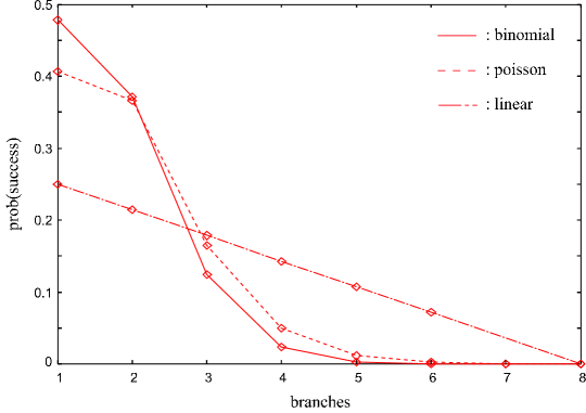
Figure 2: Probability distributions among the branches being successful.

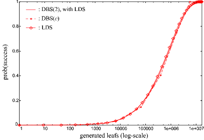
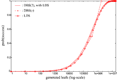
a.    linear without plateaus                        b.    linear with plateaus

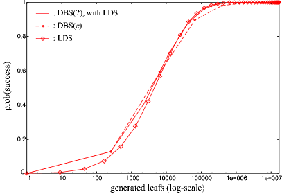
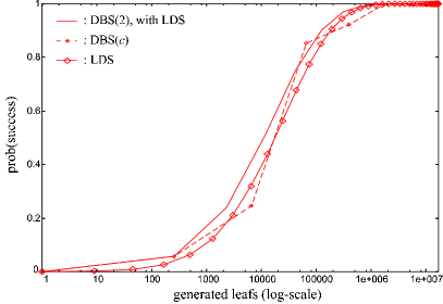
c.    poisson without plateaus                        d.    poisson with plateaus

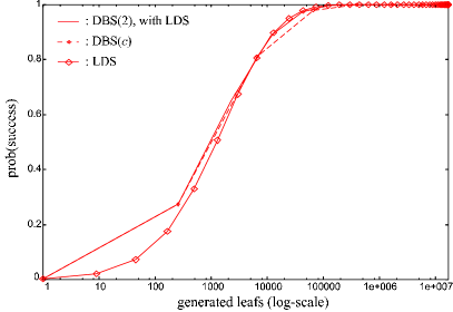
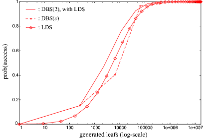
e.    binomial without plateaus                   f.    binomial with plateaus

Figure 3: Cumulative probability of success for LDS and DBS on search tree of width 8, depth 8 and linear, poisson and binomial probability distributions.

5 Computational Results

This section presents computational results of two applications for which we have compared DBS and LDS. The first is the traveling salesman problem, the second the partial latin square completion problem. For each application we state the problem, define the applied heuristic and report the computational results.

For the implementation of the applications we have used ILOG Solver [8] and Cplex [7] on a Pentium 1Ghz with 256 MB RAM.

5.1 Traveling salesman problem

The traveling salesman problem (TSP) is a traditional NP-hard combinatorial optimization problem. Given a set of cities with distances (costs) between them, the problem is to find a closed tour of minimal length visiting each city exactly once.

For the TSP, we have used a heuristic similar to the one used in [10]. It relies on the reduced cost matrix that originates from the solution of a linear relaxation (an assignment problem) inferred from the TSP. The heuristic ranks those values best that are associated to the lowest reduced costs. Intuitively this is motivated by the fact that those values will contribute the least to an optimal tour. Differently from [10] we now apply this heuristic in a dynamic way. This means that the subdomains are not selected beforehand (statically) but during the subproblem generation. This approach avoids the inclusion of already pruned domain values. Secondly, for each variable we only include values that have the same (lowest) reduced cost, instead of a range of low reduced costs.

The further tuning of DBS consists of the following. The subproblems are generated using a limited discrepancy strategy, without preference ordering concerning the discrepancies. Subproblems are being solved using depth-first search, since all leaf nodes can be considered to have equal probability of success.

To compare LDS and DBS fairly, we stop the search as soon as an optimal solution has been found. The proof of optimality should not be taken into account, because it is not directly related to the probability of a branch being successful.

	LDS			DBS
instance	time (s)	fails	discr	time (s)	fails	discr
gr17	0.08	36	2	0.02	3	0
gr21	0.16	52	3	0.01	1	0
gr24	0.49	330	5	0.01	4	0
fri26	0.16	82	2	0.01	0	0
bayg29	8.06	4412	8	0.07	82	1
bays29	2.31	1274	5	0.07	43	1
dantzig42	0.98	485	1	0.79	1317	1
swiss42	6.51	2028	4	0.08	15	0
hk48	190.96	35971	11	0.23	175	1
brazil58	N.A.	N.A.	N.A.	0.72	770	1

N.A. means ‘not applicable’ due to time limit (900 s).

Table 1: Results for finding optima of TSP instances (not proving optimality).

The results of our comparison are presented in Table 1. The instances are taken from TSPLIB [12] and represent symmetric TSPs. For LDS and DBS, the table shows the time and the number of fails (backtracks) needed to find an optimum. For LDS, the discrepancy of the leaf node that represents the optimum is given. The discrepancy of the subproblem that contains the optimum is reported for DBS.

For all instances but one, DBS performs much better than LDS. Both the number of fails and the computation time are substantially less for DBS. Observe that for the instance dantzig42 LDS needs less fails than DBS, but uses more time. Here is where the depth-first search strategy for solving the DBS subproblems pays off. It can visit almost three times more nodes in less time, because it lacks the LDS overhead.

5.2 Partial latin square completion problem

The partial latin square completion problem (PLSCP) is a well known NP-complete combinatorial satisfaction problem. A latin square is an $n\times n$ square in which each row and each column is a permutation of the numbers $\{1,\dots,n\}$. For example:

	2		4		3		1
	1		3		2		4
	4		2		1		3
	3		1		4		2

is a latin $4\times 4$ square. A partial latin square is a partially pre-assigned square. The PLSCP is the problem of extending a partial latin square to a feasible (completely filled) latin square.

As heuristic we have used a simple first-fail principle for the values, i.e. values that are most constrained are to be considered first. This means, a value that occurs the most inside a partial latin square is ranked best. Hence the rank of a value is taken equal to the number of the value’s occurrences in the partial latin square, and a higher rank is regarded better.

In our implementation, DBS groups together values of the same rank to generate subproblems, using a limited discrepancy strategy without preference ordering concerning the discrepancy. The subproblems are being solved using a depth-first strategy, since we consider all values of the same rank to be equally successful. Furthermore, the CSP that models the PLSCP uses alldifferent constraints on the rows and the columns, with maximal propagation. The maximal alldifferent propagation (achieving hyper-arc consistency) is of great importance for solving the PLSCP as a CSP. With less powerful propagation, the considered instances are practically unsolvable.

	LDS			DBS
instance	time (s)	fails	discr	time (s)	fails	discr
bpls.order25.holes238	2.36	668	5	1.09	746	5
bpls.order25.holes239	0.49	15	1	0.42	2	1
bpls.order25.holes240	1.17	179	4	0.86	893	4
bpls.order25.holes241	3.31	772	3	4.70	3123	4
bpls.order25.holes242	2.41	537	3	1.80	1753	4
bpls.order25.holes243	4.06	1082	4	3.96	2542	4
bpls.order25.holes244	1.33	214	3	2.99	2072	4
bpls.order25.holes245	9.40	2308	6	10.66	12906	7
bpls.order25.holes246	2.01	401	5	2.22	1029	4
bpls.order25.holes247	258.91	69105	6	11.66	5727	4
bpls.order25.holes248	33.65	6969	5	0.68	125	2
bpls.order25.holes249	212.76	60543	11	101.46	85533	8
bpls.order25.holes250	2.45	338	2	0.83	687	3
pls.order30.holes328	273.53	32538	4	82	14102	3
pls.order30.holes330	21.79	2756	3	25.15	5019	3
pls.order30.holes332	235.40	30033	5	56.94	9609	3
pls.order30.holes334	4.18	256	2	6.09	843	2
pls.order30.holes336	1.73	69	2	0.76	12	1
pls.order30.holes338	49.17	5069	3	29.41	8026	3
pls.order30.holes340	1.68	91	2	0.81	66	2
pls.order30.holes342	28.40	3152	3	5.41	600	2
pls.order30.holes344	9.05	605	2	8.35	1103	2
pls.order30.holes346	2.15	101	2	3.76	482	2
pls.order30.holes348	43.80	2658	2	32.86	2729	2
pls.order30.holes350	1.16	46	1	0.80	12	1
pls.order30.holes352	5.10	288	2	0.95	32	1
sum	1211.45	220793	91	396.62	159773	81
mean	46.59	8492.04	3.50	15.25	6145.12	3.12

Table 2: Results for PLS completion problems.

In Table 2 we report the performance of LDS and DBS on a set of partial latin square completion problems. The instances are generated with the PLS-generator lsencode by Gomes et al. [3]. Following remarks made in [4], our generated instances are such that they are ‘difficult’ to solve. The instances bpls.order25.holes$m$ are balanced $25\times 25$ partial latin squares, with $m$ unfilled entries (around 38%). Instances pls.order30.holes$m$ are unbalanced $30\times 30$ partial latin squares, with $m$ unfilled entries (around 38%).

Again, we report the time and the number of fails (backtracks) needed to find a solution for both LDS and DBS. The discrepancy of the leaf node that represents the solution is reported for LDS, for DBS this is the discrepancy of the subproblem that contained the solution. Although DBS performs much better than LDS on average, the results are not homogeneous. For some instances LDS even found a solution at a lower discrepancy level than DBS. This can be explained by the pruning power of the alldifferent constraint. Because DBS branches on subdomains of cardinality larger than one, the alldifferent constraint will remove less inconsistent values compared to branching on single values, as is the case with LDS. Using DBS, such values will only be removed inside the subproblems.

As was already mentioned in Section 5.1, DBS effectively exploits the depth-first strategy which it is allowed to use to solve the subproblems. For a number of instances, DBS finds a solution earlier than LDS, although making use a higher number of fails.

6 Conclusion

In this paper, we presented a theoretical and experimental evaluation of an effective search strategy, Decomposition Based Search (DBS), based on value ranking and domain partitioning. We have shown that DBS can be tuned to implement two well known search strategies, namely Iterative Broadening and Limited Discrepancy Search. Concerning IB, we show that DBS explores the same number of nodes of each IB iteration, but avoids restarts. As far as LDS is concerned, we prove that DBS has a higher probability of success on a comparable number of nodes. Experimental result on the partial latin square completion problem and on the traveling salesman problem show that DBS outperforms LDS in almost all cases.

References

- [1] F. Focacci. Solving Combinatorial Optimization Problems in Constraint Programming. PhD thesis, University of Ferrara, 2001.
- [2] M.L. Ginsberg and W.D. Harvey. Iterative broadening. Artificial Intelligence, 55(2):367–383, 1992.
- [3] C.P. Gomes, H. Kautz, and Y. Ruan. lsencode: a generator of quasigroup with holes and quasigroup completion problems, 2001.
- [4] C.P. Gomes and D. Shmoys. Completing Quasigroups or Latin Squares: A Structured Graph Coloring Problem. In Proc. Computational Symposium on Graph Coloring and Generalizations, 2002.
- [5] W. D. Harvey and M. L. Ginsberg. Limited Discrepancy Search. In C. S. Mellish, editor, Proceedings of the Fourteenth International Joint Conference on Artificial Intelligence (IJCAI-95); Vol. 1, pages 607–615, 1995.
- [6] P. van Hentenryck, L. Perron, and J.-F. Puget. Search and Strategies in OPL. ACM Transactions on Computational Logic (TOCL), 1(2):285–320, 2000.
- [7] ILOG. ILOG Cplex 7.1, Reference Manual, 2001.
- [8] ILOG. ILOG Solver 5.1, Reference Manual, 2001.
- [9] A. Lodi, M. Milano, and L.M. Rousseau. Discrepancy based additive bounding, 2003. Submitted.
- [10] M. Milano and W.J. van Hoeve. Reduced cost-based ranking for generating promising subproblems. In P. van Hentenryck, editor, Eighth International Conference on the Principles and Practice of Constraint Programming (CP’02), volume 2470 of LNCS, pages 1–16. Springer Verlag, 2002.
- [11] L. Perron. Search procedures and parallelism in constraint programming. In J. Jaffar, editor, Fifth International Conference on the Principles and Practice of Constraint Programming (CP’99), volume 1713 of LNCS, pages 346–360. Springer Verlag, 1999.
- [12] G. Reinelt. TSPLIB - a Traveling Salesman Problem Library. ORSA Journal on Computing, 3:376–384, 1991.
- [13] T. Walsh. Depth-Bounded Discrepancy Search. In Proceedings of the 15th International Joint Conference on Artificial Intelligence (IJCAI), 1997.