A Framework for High-Accuracy Privacy-Preserving Mining

Abstract

To preserve client privacy in the data mining process, a variety of techniques based on random perturbation of data records have been proposed recently. In this paper, we present a generalized matrix-theoretic model of random perturbation, which facilitates a systematic approach to the design of perturbation mechanisms for privacy-preserving mining. Specifically, we demonstrate that (a) the prior techniques differ only in their settings for the model parameters, and (b) through appropriate choice of parameter settings, we can derive new perturbation techniques that provide highly accurate mining results even under strict privacy guarantees. We also propose a novel perturbation mechanism wherein the model parameters are themselves characterized as random variables, and demonstrate that this feature provides significant improvements in privacy at a very marginal cost in accuracy.

While our model is valid for random-perturbation-based privacy-preserving mining in general, we specifically evaluate its utility here with regard to frequent-itemset mining on a variety of real datasets. The experimental results indicate that our mechanisms incur substantially lower identity and support errors as compared to the prior techniques.

1 . Introduction

The knowledge models produced through data mining techniques are only as good as the accuracy of their input data. One source of data inaccuracy is when users, due to privacy concerns, deliberately provide wrong information. This is especially common with regard to customers asked to provide personal information on web forms to e-commerce service providers.

The compulsion for doing so may be the (perhaps well-founded) worry that the requested information may be misused by the service provider to harass the customer. As a case in point, consider a pharmaceutical company that asks clients to disclose the diseases they have suffered from in order to investigate the correlations in their occurrences – for example, “Adult females with malarial infections are also prone to contract tuberculosis”. While the company may be acquiring the data solely for genuine data mining purposes that would eventually reflect itself in better service to the client, at the same time the client might worry that if her medical records are either inadvertently or deliberately disclosed, it may adversely affect her employment opportunities.

To encourage users to submit correct inputs, a variety of privacy-preserving data mining techniques have been proposed in the last few years [3, 9, 12, 18, 23]. The goal of these techniques is to keep the raw local data private but, at the same time, support accurate reconstruction of the global data mining models. Most of the techniques are based on a data perturbation approach, wherein the user data is distorted in a probabilistic manner that is disclosed to the eventual miner. For example, in the MASK technique [18], intended for privacy-preserving association-rule mining on sparse boolean databases, each $0$ or $1$ in the original user transaction vector is flipped with a parametrized probability $1-p$.

1.1 . The FRAPP Framework

The trend in the prior literature has been to propose specific perturbation techniques, which are then analyzed for their privacy and accuracy properties. We move on, in this paper, to presenting FRAPP (FRamework for Accuracy in Privacy-Preserving mining), a generalized matrix-theoretic framework that facilitates a systematic approach to the design of random perturbation schemes for privacy-preserving mining. While various privacy metrics have been discussed in the literature, FRAPP supports a particularly strong notion of privacy, originally proposed in [13]. Specifically, it supports a measure called “amplification”, which guarantees strict limits on privacy breaches of individual user information, independent of the distribution of the original data.

FRAPP quantitatively characterizes the sources of error in random data perturbation and model reconstruction processes. We first demonstrate that the prior techniques differ only in their settings for the FRAPP parameters. Further, and more importantly, we show that through appropriate choice of parameter settings, new perturbation techniques can be constructed that provide highly accurate mining results even under strict privacy guarantees. Efficient implementations for these new perturbation techniques are also presented.

We investigate here, for the first time, the possibility of randomizing the perturbation parameters themselves. The motivation is that it could lead to an increase in privacy levels since the exact parameter values used by a specific client will not be known to the data miner. This scheme has the obvious downside of perhaps reducing the model reconstruction accuracy. However, our investigation shows that the tradeoff is very attractive in that the privacy increase is substantial whereas the accuracy reduction is only marginal. This opens up the possibility of using FRAPP in a two-step process: First, given a user-desired level of privacy, identifying the deterministic values of the FRAPP parameters that both guarantee this privacy and also maximize the accuracy; and then, (optionally) randomizing these parameters to obtain even better privacy guarantees at a minimal cost in accuracy.

The FRAPP model is valid for random-perturbation-based privacy-preserving mining in general. Here, we focus on its applications to categorical databases, where the domain of each attribute is finite. Note that boolean data is a special case of this class, and further, that continuous-valued attributes can be converted into categorical attributes by partitioning the domain of the attribute into fixed length intervals.

To quantitatively evaluate FRAPP’s utility, we specifically evaluate the performance of our new perturbation mechanisms on the popular mining task of finding frequent itemsets, the cornerstone of association rule mining. Our evaluation on a variety of real datasets shows that both identity and support errors are substantially lower than those incurred by the prior privacy-preserving techniques.

1.2 . Contributions

In a nutshell, FRAPP provides a mathematical foundation for “raising both the accuracy and privacy bars in strict privacy-preserving mining”. Specifically, our main contributions are as follows:

• FRAPP, a generalized matrix-theoretic framework for random perturbation and mining model reconstruction;

• Using FRAPP to derive new perturbation mechanisms for minimizing the model reconstruction error while ensuring strict privacy guarantees;

• Introducing the concept of randomization of perturbation parameters, and thereby deriving enhanced privacy;

• Efficient implementations of the perturbation techniques for the proposed mechanisms;

• Quantitatively demonstrating the utility of our schemes in the context of association rule mining.

1.3 . Organization

The remainder of this paper is organized as follows: The FRAPP framework for data perturbation and model reconstruction is presented in Section 2. Appropriate choices of FRAPP parameters for simultaneously guaranteeing strict data privacy and providing high model accuracy are discussed in Section 3. The impact of randomizing the FRAPP parameters is investigated in Section 4. Efficient schemes for implementing the new perturbation mechanisms are described in Section 5. In Section 6, we discuss the application of our mechanisms to association rule mining. Then, in Section 7, the utility of FRAPP in the context of association rule mining is quantitatively investigated. Related work on privacy-preserving mining is reviewed in Section 8. Finally, in Section 9, we summarize the conclusions of our study and outline future research avenues.

2 . The FRAPP Framework

In this section, we describe the construction of the FRAPP framework, and its quantification of privacy and accuracy measures.

Data Model.

We assume that the original database $U$ consists of $N$ records, with each record having $M$ categorical attributes. The domain of attribute $j$ is denoted by $S_{U}^{j}$, resulting in the domain $S_{U}$ of a record in $U$ being given by $\displaystyle S_{U}={\tiny\prod}_{j=1}^{M}S_{U}^{j}$. We map the domain $S_{U}$ to index set $I_{U}=\{1,\ldots,|S_{U}|\}$, so that we can model the database as set of $N$ values from $I_{U}$. Thus, if we denote $i^{th}$ record of $U$ as $U_{i}$, we have

$$U=\{U_{i}\}_{i=1}^{N},\qquad U_{i}\in I_{U}$$

Perturbation Model

We consider the privacy situation wherein the customers trust no one except themselves, that is, they wish to perturb their records at their client site before the information is sent to the the miner, or any intermediate party. This means that perturbation is done at the level of individual customer records $U_{i}$, without being influenced by the contents of the other records in the database.

For this situation, there are two possibilities: a simple independent column perturbation, wherein the value of each attribute in the record is perturbed independently of the rest, or a more generalized dependent column perturbation, where the perturbation of each column may be affected by the perturbations of the other columns in the record. Most of the prior perturbation techniques, including [12, 13, 18], fall into the independent column perturbation category. The FRAPP framework, however, includes both kinds of perturbation in its analysis.

Let the perturbed database be $V=\{V_{1},\ldots,V_{N}\}$, with domain $S_{V}$, and corresponding index set $I_{V}$. For each original customer record $U_{i}=u,u\in I_{U}$, a new perturbed record $V_{i}=v,v\in I_{V}$ is randomly generated with probability $p(u\to v)$. Let $A$ denote the matrix of these transition probabilities, with $\displaystyle A_{vu}=p(u\to v)$. This random process maps to a Markov process, and the perturbation matrix $A$ should therefore satisfy the following properties [22]:

$$\sum_{v\in I_{V}}{A_{vu}} = 1\qquad\forall u\in I_{U}$$

$$A_{vu} \geq 0\qquad\forall u\in I_{U},v\in I_{V}$$ (1)

Due to the constraints imposed by Equation 2, the domain of $A$ is not $\mathbf{R}^{|S_{U}|\times\mathbf{|}S_{V}|}$ but a subset of it. This domain is further restricted by the choice of perturbation method. For example, for the MASK technique [18] mentioned in the Introduction, all the entries of matrix $A$ are decided by the choice of the single parameter $p$.

In this paper, we propose to explore the preferred choices of $A$ to simultaneously achieve privacy guarantees and high accuracy, without restricting ourselves ab initio to a particular perturbation method.

2.1 . Privacy Guarantees

The miner receives the perturbed database $V$ and attempts to reconstruct the original probability distribution of database $U$ using this perturbed data and the knowledge of the perturbation matrix $A$.

The prior probability of a property of a customer’s private information is the likelihood of the property in the absence of any knowledge about the customer’s private information. On the other hand, the posterior probability is the likelihood of the property given the perturbed information from the customer and the knowledge of the prior probabilities through reconstruction from the perturbed database. As discussed in [13], in order to preserve the privacy of some property of a customer’s private information, we desire that the posterior probability of that property should not be much higher than the prior probability of the property for the customer. This is quantified by saying that a perturbation method has privacy guarantees $(\rho_{1},\rho_{2})$ if, for any property $Q(U_{i})$ with prior probability less than $\rho_{1}$, the posterior probability of the property is guaranteed to be less than $\rho_{2}$.

For our formulation, we derive (using Definition 3 and Statement 1 from [13]) the following condition on the perturbation matrix $A$ in order to support $(\rho_{1},\rho_{2})$ privacy.

$$\frac{A_{vu_{1}}}{A_{vu_{2}}}\leq\gamma\leq\frac{\rho_{2}(1-\rho_{1})}{\rho_{1}(1-\rho_{2})}\qquad u_{1},u_{2}\in I_{U},\forall v\in I_{V}$$ (2)

That is, the choice of perturbation matrix $A$ should follow the restriction that the ratio of any two entries should not be more than $\gamma$.

2.2 . Reconstruction Model

We now analyze how the distribution of the original database can be reconstructed from the perturbed database. As per the perturbation model, a client $C_{i}$ with data record $U_{i}=u,u\in I_{U}$ generates record $V_{i}=v,v\in I_{V}$ with probability $p[u\rightarrow v]$. This event of generation of $v$ can be viewed as a Bernoulli trial with success probability $p[u\rightarrow v]$. If we denote outcome of $i^{th}$ Bernoulli trial by random variable $Y_{v}^{i}$, then the total number of successes $Y_{v}$ in $N$ trials is given by sum of the $N$ Bernoulli random variables. i.e.

$$Y_{v}=\sum_{i=1}^{N}{Y_{v}^{i}}$$ (3)

That is, the total number of records with value $v$ in the perturbed database will be given by the total number of successes $Y_{v}$.

Note that $Y_{v}$ is the sum of $N$ independent but non-identical Bernoulli trials. The trials are non-identical because the probability of success in a trial $i$ varies from another trial $j$ and actually depends on the values of $U_{i}$ and $U_{j}$, respectively. The distribution of such a random variable $Y_{v}$ is known as the Poisson-Binomial distribution [25].

Now, from Equation 3, the expectation of $Y_{v}$ is given by

$$E(Y_{v})=\sum_{i=1}^{N}{E(Y_{v}^{i})}=\sum_{i=1}^{N}{P(Y_{v}^{i}=1)}$$ (4)

Let $X_{u}$ denote the number of records with value $u$ in the original database. Since $P(Y_{v}^{i}=1)=p[u\rightarrow v]={A_{vu}}$, for $U_{i}=u$, we get

$$E(Y_{v})=\sum_{u\in I_{U}}A_{vu}X_{u}$$ (5)

Let $X=[{X_{1}}X_{2}\cdots{X_{|S_{U}|}}]^{T}$, $Y=[Y_{1}Y_{2}\cdots Y_{|S_{V}|}]^{T}$, then from Equation 5 we get

$$E(Y)=AX$$ (6)

We estimate $X$ as $\widehat{X}$ given by the solution of following equation

$$Y=A\widehat{X}$$ (7)

which is an approximation to Equation 6. This is a system of $|S_{V}|$ equations in $|S_{U}|$ unknowns. For the system to be uniquely solvable, a necessary condition is that the space of the perturbed database is larger than or equal to the original database (i.e. $|S_{V}|\geq|S_{U}|$). Further, if the inverse of matrix $A$ exists, then we can find the solution of above system of equations by

$$\widehat{X}=A^{-1}Y$$ (8)

That is, Equation 8 gives the estimate of the distribution of records in the original database, which is the objective of the reconstruction exercise.

2.3 . Estimation Error

To analyze the error in the above estimation process, we use the following well-known theorem from linear algebra [22]:

Theorem 1: For an equation of form $Ax=b$, the relative error in solution $x=A^{-1}b$ satisfies

$$\frac{\parallel\delta x\parallel}{\parallel x\parallel}\leq c\frac{\parallel\delta b\parallel}{\parallel b\parallel}$$

where $c$ is the condition number of matrix $A$. For a positive definite matrix, $c=\lambda_{max}/\lambda_{min}$, where $\lambda_{max}$ and $\lambda_{min}$ are the maximum and minimum eigen values of $n\times n$ matrix $A$. Informally, the condition number is a measure of stability or sensitivity of a matrix to numerical operations. Matrices with condition numbers near one are said to be well-conditioned, whereas those with condition numbers much greater than one (e.g. $10^{5}$ for a $5*5$ Hilbert matrix [22]) are said to be ill-conditioned.

From Equations 6, 8 and the above theorem, we have

$$\frac{\parallel\widehat{X}-X\parallel}{\parallel X\parallel}\leq c\frac{\parallel Y-E(Y)\parallel}{\parallel E(Y)\parallel}$$ (9)

This inequality means that the error in estimation arises from two sources: First, the sensitivity of the problem which is measured by the condition number of matrix $A$; and, second, the deviation of $Y$ from its mean as measured by the variance of $Y$.

As discussed above, $Y_{v}$ is a Poisson-Binomial distributed random variable. Hence, using the expression for variance of a Poisson-Binomial random variable [25], we can compute the variance of $Y_{v}$ to be

$$Var(Y_{v}) = A_{v}X(1-\frac{1}{N}A_{v}X)$$ (10)

$$-\sum_{u\in I_{U}}(A_{vu}-\frac{1}{N}A_{v}X)^{2}{X_{u}}$$

which depends on the perturbation matrix $A$ and the distribution $X$ of records in the original database. Thus the effectiveness of the privacy preserving method is critically dependent on the choice of matrix $A$.

3 . Choice of Perturbation Matrix

The various perturbation techniques proposed in the literature primarily differ in their choice for perturbation matrix $A$. For example,

• MASK [18] uses the matrix $A$ with

  $$A_{vu}=p^{k}(1-p)^{M_{b}-k}$$ (11)

  where $k$ is the number of attributes with matching values in perturbed value $v$ and original value $u$, $M_{b}$ is the number of boolean attributes when each categorical attribute $j$ is converted into $\mid S_{U}^{j}\mid$ boolean attributes, and $1-p$ is the value flipping probability.

• The cut-and-paste randomization operator [12] employs a matrix $A$ with

  $$A_{vu} = \sum_{z=0}^{M}p_{M}[z]\sum_{q=max\{0,z+l_{u}-M,l_{u}+l_{v}-M_{b}\}}^{min\{z,l_{u},l_{v}\}}\frac{{\binom{l_{u}}{q}}{\binom{M-l_{u}}{z-q}}}{\binom{M}{z}}$$

  $$\qquad\cdot{\binom{M_{b}-l_{u}}{l_{v}-q}}\rho^{(l_{v}-q)}(1-\rho)^{(M_{b}-l_{u}-l_{v}+q)}$$

  where (12)

  $$p_{M}[z] = \sum_{w=0}^{min\{K,z\}}{\binom{M-w}{z-w}}\rho^{(z-w)}(1-\rho)^{(M-z)}$$ (15)

  $$\cdot\left\{\begin{array}[]{ll}1-M/(K+1)&\textrm{if }w=M\textrm{ and }w<K\\ 1/(K+1)&\textrm{o.w.}\end{array}\right.$$

  Here $l_{u}$ and $l_{v}$ are the number of $1^{s}$ in the original record $u$ and its corresponding perturbed record $v$, respectively, while $K$ and $\rho$ are operator parameters.

For enforcing strict privacy guarantees, the parameters for the above methods are decided by the constraints on the values of perturbation matrix $A$ given in Equation 2. It turns out that for practical values of privacy requirements, the resulting matrix $A$ for these schemes is extremely ill-conditioned – in fact, we found the condition numbers in our experiments to be of the order of $10^{5}$ and $10^{7}$ for MASK and the Cut-and-Paste operator, respectively.

Such ill-conditioned matrices make the reconstruction very sensitive to the variance in the distribution of the perturbed database. Thus, it is important to carefully choose the matrix $A$ such that it is well-conditioned (i.e has a low condition number). If we decide on a distortion method apriori, as in the prior techniques, then there is little room for making specific choices of perturbation matrix $A$. Therefore, we take the opposite approach of first designing matrices of the required type, and then devising perturbation methods that are compatible with the chosen matrices.

To choose the appropriate matrix, we start from the intuition that for $\gamma=\infty$, the matrix choice would be the unity matrix, which satisfies the constraints on matrix $A$ imposed by Equations 2 and 2, and has condition number 1. Hence, for a given $\gamma$, we can choose the following matrix:

$$A_{ij}=\left\{\begin{array}[]{ll}\gamma x,&\textrm{if }i=j\\ x,&\textrm{o.w.}\end{array}\right.$$ (17)

$$where$$

$$x=\frac{1}{\gamma+(|S_{U}|-1)}$$ (18)

This matrix will be of the form

$$\begin{array}[]{cc}x&\left[\begin{array}[]{cccc}\gamma&1&1&\ldots\\ 1&\gamma&1&\ldots\\ 1&1&\gamma&\ldots\\ \vdots&\vdots&\vdots&\ddots\end{array}\right]\end{array}$$

It is easy to see that the above matrix, which incidentally is a symmetric Toeplitz matrix [22], satisfies the conditions given by Equations 2 and 2. Further, its condition number can be computed to be $1+\frac{\mid S_{U}\mid}{\gamma-1}$, For ease of exposition, we will hereafter refer to this matrix informally as the “gamma-diagonal matrix”.

At this point, an obvious question is whether it is possible to design matrices that have even lower condition number than the gamma-diagonal matrix. In the remainder of this section, we prove that within the constraints of our problem, the gamma-diagonal matrix has the lowest possible condition number, that is, it is an optimal choice (albeit non-unique).

Proof.

To prove this, we will first derive the expression for minimum condition number for such matrices and the conditions under which that condition number is achieved. Then we show that our gamma-diagonal matrix satisfies these conditions, and has minimum condition number.

For a symmetric positive definite matrix, the condition number is given by

$$c = \frac{\lambda_{max}}{\lambda_{min}}$$ (19)

where $\lambda_{max}$ and $\lambda_{min}$ are the maximum and minimum eigenvalues of the matrix. As the matrix $A$ is a Markov matrix (refer Equation 2), the following theorem for eigenvalues of a matrix can be used

Theorem 2 [22] For an $n\times n$ Markov matrix,

• $1$ is an eigenvalue

• the other eigenvalues satisfy $\mid\lambda_{i}\mid\leq 1$

Theorem 3 [22] The sum of $n$ eigenvalues equals the sum of $n$ diagonal entries:

$$\lambda_{1}+\cdots+\lambda_{n}=A_{11}+\cdots+A_{nn}$$

Using Theorem 2 we get,

$$\lambda_{max} = 1$$

As the least eigenvalue $\lambda_{min}$ will always be less than or equal to average of the eigenvalues other than $\lambda_{max}$, we get,

$$\lambda_{min} \leq \frac{1}{n-1}{\sum_{i=2}^{n}\lambda_{i}}$$

where $\lambda_{1}=\lambda_{max}$ Using Theorem 3,

$$\lambda_{min} \leq \frac{1}{n-1}\Bigg{(}\sum_{i=1}^{n}A_{ii}-1\Bigg{)},$$ (20)

Hence, condition number,

$$c=\frac{1}{\lambda_{min}}\geq\frac{n-1}{\sum_{i=1}^{n}A_{ii}-1}$$ (21)

Now, due to privacy constraints on $A$ given by Equation 2,

$$A_{ii}\leq\gamma A_{ij}\textrm{ for any }j\neq i,$$

i.e.,

$$\begin{array}[]{ccc}A_{ii}&\leq&\gamma A_{i1}\\ A_{ii}&\leq&\gamma A_{i2}\\ {}\hfil&\vdots&{}\hfil\end{array}$$

Summing above,

$$(n-1)A_{ii} \leq \gamma\sum_{j\neq i}A_{ij}$$

$$= \gamma(1-A_{ii})$$

where the last step is due to the condition on $A$ given by Equation 2. Solving for $A_{ii}$, we get,

$$A_{ii} \leq \frac{\gamma}{\gamma+n-1}$$ (22)

Using above inequality in Equation 21, we get

$$c\geq\frac{n-1}{\frac{n\gamma}{\gamma+n-1}-1}=\frac{\gamma+n-1}{\gamma-1}$$ (23)

Hence minimum condition number for the symmetric perturbation matrices under privacy constraints represented by $\gamma$ is $\frac{\gamma+n-1}{\gamma-1}$. This condition number is achieved when $A_{ii}=\frac{\gamma}{\gamma+n-1}$.

The diagonal values of gamma-diagonal matrix given by Equation 2 is $\frac{\gamma}{\gamma+n-1}$. Thus it is minimum condition number symmetric perturbation matrix, with condition number $\frac{\gamma+\mid S_{U}\mid-1}{\gamma-1}$.

4 . Randomizing the Perturbation Matrix

The estimation model in the previous section implicitly assumed the perturbation matrix $A$ to be deterministic. However, it appears intuitive that if the perturbation matrix parameters are themselves randomized, so that each client uses a perturbation matrix that is not specifically known to the miner, the privacy of the client will be further increased. Of course, it may also happen that the reconstruction accuracy may suffer in this process.

In this section, we explore this tradeoff. Instead of deterministic matrix $A$, the perturbation matrix here is matrix $\tilde{A}$ of random variables, where each entry $\tilde{A}_{vu}$ is a random vaiable with $E(\tilde{A}_{vu})=A_{vu}$. The values taken by the random variables for a client $C_{i}$ provide the specific values for his/her perturbation matrix.

4.1 . Privacy Guarantees

Let $Q(U_{i})$ be a property of client $C_{i}$’s private information, and let record $U_{i}=u$ be perturbed to $V_{i}=v$. Denote the prior probability of $Q(U_{i})$ by $P(Q(U_{i}))$. On seeing the perturbed data, the posterior probability of the property is calculated to be:

$$P(Q(U_{i})|V_{i}=v) = \sum_{Q(u)}P_{U_{i}|V_{i}}(u|v)$$

$$= \sum_{Q(u)}\frac{P_{U_{i}}(u)P_{V_{i}|U_{i}}(v|u)}{P_{V_{i}}(v)}$$

When we use a fixed perturbation matrix $A$ for all clients $i$, then $P_{V_{i}/U_{i}}(v/u)=A_{vu},\forall i$. Hence

$$P(Q(U_{i})|V_{i}=v) = \frac{\sum_{Q(u)}P_{U_{i}}(u)A_{vu}}{\sum_{Q(u)}P_{U_{i}}(u)A_{vu}+\sum_{\neg Q(u)}P_{U_{i}}(u)A_{vu}}$$

As discussed in [13], the data distribution $P_{U_{i}}$ in the worst case can be such that $P(U_{i}=u)>0$ only if $\{u\in I_{U}|Q(u)\textrm{ and }A_{vu}=maxp\}$
or
$\{u\in I_{U}|\neg Q(u)\textrm{ and }A_{vu}=minp\}$,
so that

$$P(Q(U_{i})/V_{i}=v)=\frac{P(Q(u))\cdot maxp}{P(Q(u))\cdot maxp+P(\neg Q(u))\cdot minp}$$

where $maxp=\max_{Q(u^{\prime})}A_{vu^{\prime}}$ and $minp=\min_{\neg Q(u^{\prime})}A_{vu^{\prime}}$. Since the distribution $P_{U}$ is known through reconstruction to the miner, and matrix $A$ is fixed, the above posterior probability can be determined by the miner. For example, if $P(Q(u))=5\%,\gamma=19$, the posterior probability can be computed to be $50\%$ for perturbation with the gamma-diagonal matrix.

But, in the randomized matrix case where $P_{V_{i}/U_{i}}(v/u)$ is a realization of random variable $\tilde{A}$, only its distribution and not the exact value for a given $i$ is known to the miner. Thus determinations like the above cannot be made by the miner for a given record $U_{i}$. For example, suppose we choose matrix $A$ such that

$$A_{uv}=\left\{\begin{array}[]{ll}\gamma x+r,&\textrm{if }u=v\\ x-\frac{r}{\mid S_{U}\mid-1},&\textrm{o.w.}\end{array}\right.$$ (25)

where $x=\frac{1}{\gamma+(|S_{U}|-1)}$ and $r$ is a random variable uniformly distributed between $[-\alpha,\alpha]$. Thus, the worst case posterior probability for a record $U_{i}$ is now a function of the value of $r$, and is given by

$$\rho_{2}(r)=\frac{P(Q(u))\cdot\gamma x+r}{P(Q(u))\cdot(\gamma x+r)+P(\neg Q(u))(x-\frac{r}{\mid S_{U}\mid-1})}$$

Therefore, only the posterior probability range, i.e. $[\rho_{2}^{-},\rho_{2}^{+}]=[\rho_{2}(-\alpha),\rho_{2}(+\alpha)]$, and the distribution over the range, can be determined by the miner. For example, for the situation $P(Q(u))=5\%,\gamma=19,\alpha=\gamma x/2$, he can only say that the posterior probability lies in the range [$33\%,60\%$] with its probability of being greater than 50% ($\rho_{2}$ corresponding to $r=0$) equal to its probability of being less than 50%.

4.2 . Reconstruction Model

The reconstruction model for the deterministic perturbation matrix $A$ was discussed in Section 2.2. We now describe the changes to this analysis for the randomized perturbation matrix $\tilde{A}$.
The probability of success for Bernoulli variable $Y_{v}^{i}$ is now modified to

$$P(Y_{v}^{i}=1)=\tilde{A}_{vu}^{i},\textrm{ for }U_{i}=u$$

where $\tilde{A}_{vu}^{i}$ denotes the $i^{th}$ realization of random variable $\tilde{A}_{vu}$.

Thus, from Equation 4,

$$E(Y_{v}) = \sum_{i=1}^{N}{P(Y_{v}^{i}=1)}$$ (26)

$$= \sum_{u\in I_{U}}{\sum_{\{i|U_{i}=u\}}{{\tilde{A}}_{vu}^{i}}}$$

$$= \sum_{u\in I_{U}}{\overline{A}_{vu}{X_{u}}}$$

$$\Rightarrow E(Y) = \overline{A}_{vu}X$$ (27)

where $\overline{A}_{vu}=\frac{1}{{X_{u}}}\sum_{\{i|U_{i}=u\}}{\tilde{A}_{vu}^{i}}$ is the average of the values taken by $\tilde{A}_{vu}$ for the clients whose original data record had value $u$.

$\tilde{A}_{vu}$ is a random variable with expectation $E(\tilde{A}_{vu})=A_{vu}$, it can be easily seen that,

$$E(\overline{A}_{vu})=A_{vu}$$ (28)

Hence, from Equation 26, we get

$$E(E(Y))=AX$$ (29)

We estimate $X$ as $\widehat{X}$ given by the solution of following equation

$$Y=A\widehat{X}$$ (30)

which is an approximation to Equation 29. From Theorem 1 in Section 2.2, the error in estimation is bounded by:

$$\frac{\parallel\widehat{X}-{X}\parallel}{\parallel X\parallel}\leq c\frac{\parallel Y-E(E(Y))\parallel}{\parallel E(E(Y))\parallel}$$ (31)

where $\boldmath{c}$ is the condition number of perturbation matrix $A$.

We now compare these bounds with the corresponding bounds of the deterministic case. Firstly, note that, due to the use of the randomized matrix, there is a double expectation for $Y$ on the RHS of the inequality, as opposed to the single expectation in the deterministic case. Secondly, only the numerator is different between the two cases since $E(E(Y))=AX$. Now, we have

$${}\parallel Y-E(E(Y))\parallel$$

$$= \parallel(Y-E(Y))+(E(Y)-E(E(Y)))\parallel$$

$$\leq \parallel Y-E(Y)\parallel+\parallel E(Y)-E(E(Y))\parallel$$

Here $\parallel Y-E(Y)\parallel$ is given by the variance of random variable $Y$. Since $Y_{v}$, as discussed before, is Poisson-binomial distributed, its variance is given by [25]

$$Var(Y_{v}) = N\overline{p}_{v}-\sum_{i}{(p_{v}^{i})^{2}}$$ (32)

where $\overline{p}_{v}=\frac{1}{N}\sum_{i}{p_{v}^{i}}$ and $p_{v}^{i}=P(Y_{v}^{i}=1)$.

It is easily seen (by elementary calculus or induction) that among all combinations $\{p_{v}^{i}\}$ such that $\sum_{i}{p_{v}^{i}}=n\overline{p}_{v}$, the sum $\sum_{i}{(p_{v}^{i})^{2}}$ assumes its minimum value when all $p_{v}^{i}$ are equal. It follows that, if the average probability of success $\overline{p}_{v}$ is kept constant, $Var(Y_{v})$ assumes its maximum value when $p_{v}^{1}=\cdots=p_{v}^{N}$. In other words, the variability of $p_{v}^{i}$, or its lack of uniformity, decreases the magnitude of chance fluctuations, as measured by its variance [14]. On using random matrix $\tilde{A}$ instead of deterministic $A$ we increase the variability of $p_{v}^{i}$ (now $p_{v}^{i}$ assumes variable values for all $i$), hence decreasing the fluctuation of $Y_{v}$ from its expectation, as measured by its variance.

Hence, $\parallel Y-E(Y)\parallel$ is likely to be decreased as compared to the deterministic case, thereby reducing the error bound. On the other hand, the positive value $\parallel E(Y)-E(E(Y))\parallel=\parallel(\overline{A}-A)X\parallel$, which depends upon the variance of the random variables in $\tilde{A}$, was $0$ in the deterministic case. Thus, the error bound is increased by this term.

So, we have a classic tradeoff situation here, and as shown later in our experiments of Section 7, the tradeoff turns out very much in our favour with the two opposing terms almost canceling each other out, making the error only marginally worse than the deterministic case.

5 . Implementation of Perturbation Algorithm

To implement the perturbation process discussed in the previous sections, we effectively need to generate for each $U_{i}=u$, a discrete distribution with PMF $P(v)=A_{vu}$ and CDF $F(v)=\sum_{i\leq v}A_{iu}$, defined over $v=1,\ldots,\mid S_{V}\mid$.

A straightforward algorithm for generating the perturbed record $v$ from the original record $u$ is the following

1. Generate $r\sim{\cal U}(0,1)$

2. Repeat for $v=1,\ldots,\mid S_{V}\mid$

   if $F(v-1)<r\leq F(v)$

   return $V_{i}=v$

where ${\cal U}(0,1)$ denotes uniform distribtion over range $[0,1]$

This algorithm, whose complexity is proportional to the product of the cardinalities of the attribute domains, will require $\mid S_{V}\mid/2$ iterations on average which can turn out to be very large. For example, with $31$ attributes, each with two categories, this amounts to $2^{30}$ iterations for each customer! We therefore present below an alternative algorithm whose complexity is proportional to the sum of the cardinality of the attribute domains.

Given that we want to perturb the record $U_{i}=u$, we can write

$$\begin{array}[]{l}P(V_{i};U_{i}=u)\\ =P(V_{i1},\ldots,V_{iM};u)\\ =P(V_{i1};u)\cdot P(V_{i2}|V_{i1};u)\cdots P(V_{iM}|V_{i1},\ldots,V_{i(M-1)};u)\end{array}$$

For the perturbation matrix $A$, we get the following expressions for the above probabilities:

$$P(V_{i1}=a;u) = \sum_{\{v|v(1)=a\}}{A_{vu}}$$

$$P(V_{i2}=b|V_{i1}=a;u) = \frac{P(V_{i2}=b,V_{i1}=a;u)}{P(V_{i1}=a);u}$$

$$= \frac{\sum_{\{v|v(1)=a\&v(2)=b\}}{A_{vu}}}{P(V_{i1}=a;u)}$$

$$\ldots\textrm{and so on }$$

where $v(i)$ denotes value of $i^{th}$ column for record value =$v$.

For the gamma-diagonal matrix $A$, and using $n_{j}$ to represent $\prod_{k=1}^{j}{\mid S_{U}^{k}\mid}$, we get the following expressions for these probabilities after some simple algebraic calculations:

$$P(V_{i1}=b;U_{i1}=b) = (\gamma+\frac{n_{M}}{n_{1}}-1)x$$

$$P(V_{i1}=b;U_{i1}\neq b) = \frac{n_{M}}{n_{1}}x$$

Then, for the $j^{th}$ attribute

$$P(V_{ij}/V_{i1},\ldots,V_{i(j-1)};U_{i})\qquad\qquad\qquad\qquad\qquad$$

$$=\left\{\begin{array}[]{ll}\frac{(\gamma+\frac{n_{M}}{n_{j}}-1)x}{\prod_{k=1}^{j-1}p_{k}},&\qquad\textrm{if }\forall k\leq j,V_{ik}=U_{ik}\\ \\ \frac{(\frac{n_{M}}{n_{j}})x}{\prod_{k=1}^{j-1}p_{k}},&\qquad\textrm{o.w.}\\ \end{array}\right.$$ (36)

where $p_{k}$ is the probability that $V_{ik}$ takes value $a$, given that $a$ is the outcome of the random process performed for $k^{th}$ attribute. i.e.

$$p_{k}=P(V_{ik}=a/V_{i1},\ldots,V_{i(k-1)};U_{i})$$

Therefore, to achieve the desired random perturbation for a value in column $j$, we use as input both its original value and the perturbed value of the previous column $j-1$, and generate the perturbed value as per the discrete distribution given in Equation 5. Note that is an example of dependent column perturbation, in contrast to the independent column perturbation used in most of the prior techniques.

To assess the complexity, it is easy to see that the average number of iterations for the $j^{th}$ discrete distribution will be ${\small|S_{U}^{j}|/2}$, and hence the average number of iterations for generating a perturbed record will be ${\small\sum_{j}|S_{U}^{j}|/2}$ (this value turns out to be exactly $M$ for a boolean database).

6 . Application to Association Rule Mining

To illustrate the utility of the FRAPP framework, we demonstrate in this section how it can be used for enhancing privacy-preserving mining of association rules, a popular mining model that identifies interesting correlations between database attributes [1, 21].

The core of the association rule mining is to identify “frequent itemsets”, that is, all those itemsets whose support (i.e. frequency) in the database is in excess of a user-specified threshold. Equation 8 can be directly used to estimate the support of itemsets containing all $M$ categorical attributes. However, in order to incorporate the reconstruction procedure into bottom-up association rule mining algorithms such as Apriori [2], we need to also be able to estimate the supports of itemsets consisting of only a subset of attributes.

Let $C$ denotes the set of all attributes in the database, and $C_{s}$ be a subset of attributes. Each of the attributes $j\in C_{s}$ can assume one of the $|S_{U}^{j}|$ values. Thus, the number of itemsets over attributes in $C_{s}$ is given by $n_{C_{s}}=\prod_{j\in{C_{s}}}|S_{U}^{j}|$. Let ${\cal L,H}$ denote itemsets over this subset of attributes.

We say that record supports an itemset $\cal L$ over $C_{s}$ if the entries in the record for the attributes $j\in C_{s}$ are same as in $\cal L$.

Let support of an itemset ${\cal L}$ in original and distorted database be denoted by $sup^{U}_{{\cal L}}$ and $sup^{V}_{{\cal L}}$, respectively. Then,

$$sup^{V}_{{\cal L}} = \frac{1}{N}\sum_{v\textrm{\tiny{ supports }}{\cal L}}Y_{v}$$

where $Y_{v}$ denotes the number of records in $V$ with value $v$ (refer Section 2.2). From Equation 7, we know

$$Y_{v} = \sum_{u\in I_{U}}A_{vu}\widehat{X}_{u}$$ (38)

Hence,

$$sup^{V}_{{\cal L}} = \frac{1}{N}\sum_{v\textrm{\tiny{ supports }}{\cal L}}\sum_{u}A_{vu}\widehat{X}_{u}$$

$$= \frac{1}{N}\sum_{u}\widehat{X}_{u}\sum_{v\textrm{\tiny{ supports }}{\cal L}}A_{vu}$$

$$= \frac{1}{N}\sum_{{\cal H}}\sum_{u\textrm{\tiny{ supports }}{\cal H}}\widehat{X}_{u}\sum_{v\textrm{\tiny{ supports }}{\cal L}}A_{vu}$$

If for all $u$ which support a given itemset ${\cal H}$, $\sum_{v\textrm{\tiny{ supports }}{\cal L}}A_{vu}={\cal A}_{\cal HL}$, i.e. it is equal for all $u$ which support a given itemset, then the above equation can be written as:

$$sup^{V}_{{\cal L}} = \frac{1}{N}\sum_{{\cal H}}{\cal A}_{{\cal HL}}\sum_{u\textrm{\tiny{ supports }}{\cal H}}\widehat{X}_{u}$$

$$= \sum_{{\cal H}}{\cal A}_{{\cal HL}}\qquad\widehat{sup^{U}}_{{\cal H}}$$

Now we find the matrix ${\cal A}$ for our gamma-diagonal matrix. Through some simple algebra, we get following matrix $\cal A$ corresponding to itemsets over subset $C_{s}$, Hence,

$${\cal A}_{\cal HL}=\left\{\begin{array}[]{ll}\gamma x+(\frac{n_{C}}{n_{C_{s}}}-1)x,&\textrm{if }{\cal H=L}\\ \frac{n_{C}}{n_{C_{s}}}x,&\textrm{o.w.}\end{array}\right.$$ (40)

Using the above $n_{C_{s}}\times n_{C_{s}}$ matrix we can estimate support of itemsets over any subset $C_{s}$ of attributes. Thus our scheme can be implemented on popular bottom-up association rule mining algorithms.

7 . Performance Analysis

We move on, in this section, to quantify the utility of the FRAPP framework with respect to the privacy and accuracy levels that it can provide for mining frequent itemsets.

Table 1: CENSUS Dataset

Attribute	Categories
age	$(15-35],(35-55],(55-75],>75$
fnlwgt	$(0-1e5],(1e5-2e5],(1e5-3e5],(3e5-4e5],>4e5$
hours-per-week	$(0-20],(20-40],(40-60],(60-80],>80$
race	White, Asian-Pac-Islander, Amer-Indian-Eskimo, Other, Black
sex	Female, Male
native-country	United-States, Other

Table 2: HEALTH Dataset

Attribute	Categories
AGE (Age)	$[0-20),[20-40),[40-60),[60-80),\geq 80)$
BDDAY12 (Bed days in past 12 months)	$[0-7),[7-15),[15-30),[30-60),\geq 60$
DV12 (Doctor visits in past 12 months)	$[0-7),[7-15),[15-30),[30-60),\geq 60$
PHONE (Has Telephone)	Yes,phone number given; Yes, no phone number given; No
SEX (Sex)	Male ; Female
INCFAM20 (Family Income)	Less than $20,000; $20,000 or more
HEALTH (Health status)	Excellent; Very Good; Good; Fair; Poor

Datasets.

We use the following real world datasets in our experiments:

CENSUS

: This dataset contains census information for approximately 50,000 adult American citizens. It is available from the UCI repository [26], and is a popular benchmark in data mining studies. It is also representative of a database where there are fields that users may prefer to keep private – for example, the “race” and “sex” attributes. We use three continuous (age, fnlwgt, hours-per-week) and three nominal attributes (native-country, sex, race) from the census database in our experiments. The continuous attributes are partitioned into (five) equiwidth intervals to convert them into categorical attributes. The categories used for each attribute are listed in Table 1.

HEALTH

: This dataset captures health information for over 100,000 patients collected by the US government [27]. We selected 3 continuous and 4 nominal attributes from the dataset for our experiments. The continuous attributes were partitioned into equi-width intervals to convert them into categorical attributes. The attributes and their categories are listed in Table 2.

We evaluated the association rule mining accuracy of our schemes on the above datasets for $sup_{min}=2\%$. Table 3 gives the number of frequent itemsets in the datasets for $sup_{min}=2\%$.

Table 3: Frequent Itemsets for $sup_{min}=0.02$

	Itemset Length
	1	2	3	4	5	6	7
CENSUS	19	102	203	165	64	10	–
HEALTH	23	123	292	361	250	86	12

Privacy Metric.

The $(\rho_{1},\rho_{2})$ strict privacy measure from [13] is used as the privacy metric. While we experimented with a variety of privacy settings, due to space limitations, we present results here for a sample $(\rho_{1},\rho_{2})=(5\%,50\%)$, which was also used in [13]. This privacy value results in $\gamma=19$.

Accuracy Metrics.

We evaluate two kinds of mining errors, Support Error and Identity Error, in our experiments:

Support Error ($\rho$)

This metric reflects the (percentage) average relative error in the reconstructed support values for those itemsets that are correctly identified to be frequent. Denoting the number of frequent itemsets by $|F|$, the reconstructed support by $\widehat{sup}$ and the actual support by $sup$, the support error is computed over all frequent itemsets as

$${\rho}=\frac{1}{\mid F\mid}\Sigma_{f\in F}\frac{\mid\widehat{sup}_{f}-sup_{f}\mid}{sup_{f}}*100$$

Identity Error ($\sigma$)

This metric reflects the percentage error in identifying frequent itemsets and has two components: $\sigma^{+}$, indicating the percentage of false positives, and $\sigma^{-}$ indicating the percentage of false negatives. Denoting the reconstructed set of frequent itemsets with $R$ and the correct set of frequent itemsets with $F$, these metrics are computed as:

${\sigma^{+}}=\frac{\mid R-F\mid}{\mid F\mid}*100$             ${\sigma^{-}}=\frac{\mid F-R\mid}{\mid F\mid}$ * 100

Perturbation Mechanisms.

We show frequent-itemset-mining accuracy results for our proposed perturbation mechanisms as well as representative prior techniques. For all the perturbation mechanisms, the mining from the distorted database was done using Apriori [2] algorithm, with an additional support reconstruction phase at the end of each pass to recover the original supports from the perturbed database supports computed during the pass [18, 8].

The perturbation mechanisms evaluated in our study are the following:

DET-GD:

This schemes uses the deterministic gamma-diagonal perturbation matrix $A$ (Section 3) for perturbation and reconstruction. The implementation described in Section 5 was used to carry out the perturbation, and the results of Section 6 were used to compute the perturbation matrix used in each pass of Apriori for reconstruction.

RAN-GD:

This scheme uses the randomized gamma-diagonal perturbation matrix $\tilde{A}$ (Section 4) for perturbation and reconstruction. Though in general, any distribution can be used for $\tilde{A}$, here we evaluate the performance of uniformly distributed $\tilde{A}$ given by Equation 25 over the entire range of the randomization parameter $\alpha$.

MASK:

This is the perturbation scheme proposed in [18], which is intended for boolean databases and is characterized by a single parameter $1-p$, which determines the probability of an attribute value being flipped. In our scenario, the categorical attributes are mapped to boolean attributes by making each value of the category an attribute. Thus, the $M$ categorical attributes map to $M_{b}=\sum_{j}\mid S_{U}^{j}\mid$ boolean attributes.

The flipping probability $1-p$ was chosen as the lowest value which could satisfy the constraints given by Equation 2. The constraint $\forall v:\forall u_{1},u_{2}:\frac{A_{vu_{1}}}{A_{vu_{2}}}\leq\gamma$ is satisfied for MASK [18], if $\displaystyle\frac{p^{M_{b}}}{(1-p)^{M_{b}}}\leq\gamma$. But, for each categorical attribute, one and only one of its associated boolean attributes takes value $1$ in a particular record. Therefore, all the records contain exactly $M$ $1^{s}$, and the following condition is sufficient for the privacy constraints to be satisfied:

$$\frac{p^{2M}}{(1-p)^{2M}}\leq\gamma$$

. This equation was used to determine the appropriate value of $p$. Value of $p$ turns out be $0.5610$ and $0.5524$ respectively for CENSUS and HEALTH datasets for $\gamma=19$.

C&P:

This is the Cut-and-Paste perturbation scheme proposed in [12], with algorithmic parameters $K$ and $\rho$. To choose $K$, we varied $K$ from $0$ to $M$, and for each $K$, $\rho$ was chosen such that the matrix (Equation • ‣ 3) satisfies the privacy constraints (Equation 2). The results reported here are for the $(K,\rho)$ combination giving the best mining accuracy. For $\gamma=19$ $K=3,\rho=0.494$ turn out to be appropriate values.

7.1 . Experimental Results

For the CENSUS dataset, the support ($\rho$) and identity ($\sigma^{-}$, $\sigma^{+}$) errors of the four perturbation mechanisms (DET-GD, RAN-GD, MASK, C&P) is shown in Figure 1, as a function of the length of the frequent itemsets. The corresponding graphs for the HEALTH dataset are shown in Figure 2. In this graph for comparison, the performance of RAN-GD is shown for randomization parameter $\alpha={\gamma x}/{2}$. Note that the support error ($\rho$) is plotted on a log-scale.

In these figures, we first note that the performance of the DET-GD method is visibly better than that of MASK and C&P. In fact, as the length of the frequent itemset increases, the performance of both MASK and C&P degrades drastically. MASK is not able to find any itemsets of length above 4 for the CENSUS dataset, and above 5 for the HEALTH dataset, while C&P does not works after 3-length itemsets.

The second point to note is that the accuracy of RAN-GD, although dealing with a randomized matrix, is only marginally lower than that of DET-GD. In return, it provides a substantial increase in the privacy – its worst case (determinable) privacy breach is only $33\%$ as compared to $50\%$ with DET-GD. Figure 3 shows performance of RAN-GD over entire range of $\alpha$, and the posterior probability range $[\rho^{-},\rho^{+}]$. It shows mining support reconstruction errors for itemset length $4$. We can observe that the performance of RAN-GD does not deviate much from the derterministic case over the entire range, where as very low determinable posterior probability can be obtained for higher values of $\alpha$.

The primary reason for DET-GD and RAN-GD’s good performance is the low condition number of their perturbation matrices. This is quantitatively shown in Figure 4, which compares the condition numbers (on a log-scale) of the reconstruction matrices. Note that as the expected value of random matrix $\tilde{A}$ is used for estimation in RAN-GD, and the random matrix used in experiments has expected value $A$ (refer Equation 25) used in DET-GD, the condition numbers for two methods are equal. Here we see that the condition number for DET-GD and RAN-GD is not only low but also constant over all lengths of frequent itemsets (as mentioned before, the condition number is equal to $1+\frac{|S_{U}|)}{(\gamma-1)}$). In marked contrast, the condition number for MASK and C&P increase exponentially with increasing itemset length, resulting in drastic degradation in accuracy. Thus our choice of a gamma-diagonal matrix shows highly promising results for discovery of long patterns.

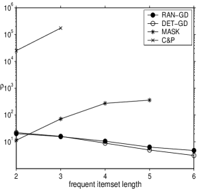
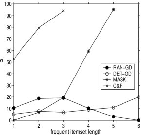
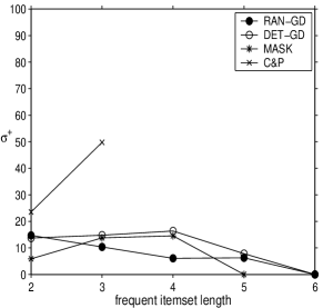
Figure 1: (a) Support error $\rho$ (b) False negatives $\sigma^{-}$ (c) False positives $\sigma^{+}$ for CENSUS dataset

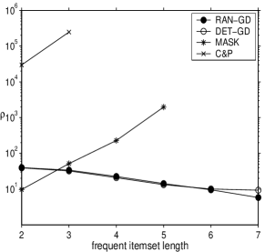
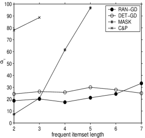
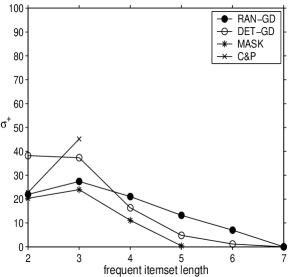
Figure 2: (a) Support error $\rho$ (b) False negatives $\sigma^{-}$ (c) False positives $\sigma^{+}$ for HEALTH dataset

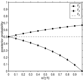
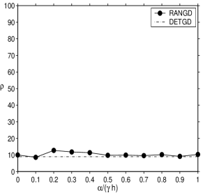
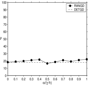
Figure 3: (a) Posterior probability ranges (b) Support error $\rho$ for CENSUS (c) Support error $\rho$ for HEALTH dataset with varying degree of randomization

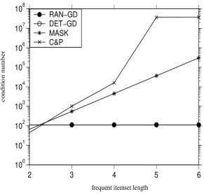
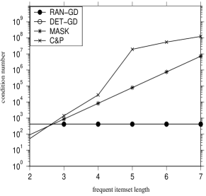
Figure 4: Comparison of condition number of transition probability matrix (a) CENSUS (b) HEALTH

8 . Related Work

The issue of maintaining privacy in data mining has attracted considerable attention in the recent past.

The work closest to our approach is that of [3, 7, 12, 18, 13]. In the pioneering work of [3], privacy-preserving data classifiers based on adding noise to the record values were proposed. This work was extended in [7] and [16] to address a variety of subtle privacy loopholes.

New randomization operators for maintaining data privacy for boolean data were presented and analyzed in [12, 18]. These methods are for categorical/boolean data and are based on probabilistic mapping from domain space to the range space rather than by incorporating additive noise to continuous valued data. A theoretical formulation of privacy breaches for such methods and a methodology for limiting them were given in the foundational work of [13].

Our work is directly related to the above-mentioned methodologies for privacy preserving mining. We combine the approaches for random perturbation on categorical data into a common theoretical framework, and explore how well random perturbation methods can do in the face of strict privacy requirements. We show that we can derive a perturbation matrix which performs significantly better than the existing methods for discovery of frequent itemsets in categorical data while simultaneously ensuring strict privacy guarantees. Also, we propose the novel idea of making the perturbation matrix itself random which, to the best of our knowledge, has not been previously explored in the context of privacy preserving mining.

Another model of privacy preserving data mining is k-anonymity model [23]. The perturbation approach used in random perturbation model works under the strong privacy requirement that even the dataset forming server is not allowed to learn or recover precise records. Users trust nobody and perturb their record at their end before providing it to any other party. k-anonymity model[23] does not satisfy this requirements. The condensation approach discussed in [9] also requires the relaxation of the assumption that even the data forming server is not allowed to learn or recover records, as in k-anonymity model. Hence these models are orthogonal to our privacy model.

[6, 4, 17, 5] deal with Hippocratic databases which are the database systems that take responsibility of the privacy of data they manage. It involves specification of how the data is to be used in a privacy policy and enforcing limited disclosure rules for regulatory concerns prompted by legislation.

Finally, the problem addressed in [19, 10, 11, 20] is how to prevent sensitive rules from being inferred by the data miner – this work is complementary to ours since it addresses concerns about output privacy, whereas our focus is on the privacy of the input data. Maintaining input data privacy is considered in [24, 15, clif03, clif04] in the context of databases that are distributed across a number of sites with each site only willing to share data mining results, but not the source data.

9 . Conclusions and Future Work

In this paper, we developed FRAPP, a generalized model for random-perturbation-based methods operating on categorical data under strict privacy constraints. We showed that by making careful choices of the model parameters and building perturbation methods for these choices, order-of-magnitude improvements in accuracy could be achieved as compared to the conventional approach of first deciding on a method and thereby implicitly fixing the associated model parameters. In particular, we proved that a “gamma-diagonal” perturbation matrix is capable of delivering the best accuracy, and is in fact, optimal with respect to its condition number. We presented an implementation technique for gamma-diagonal-based perturbation, whose complexity is proportional to the sum of the domain cardinalities of the attributes in the database. Empirical evaluation of our new gamma-diagonal-based techniques on the CENSUS and HEALTH datasets showed substantial reductions in frequent itemset identity and support reconstruction errors.

We also investigated the novel strategy of having the perturbation matrix composed of not values, but random variables instead. Our analysis of this approach showed that, at a marginal cost in accuracy, signficant improvements in privacy levels could be achieved.

In our future work, we plan to extend our modeling approach to other flavors of mining tasks.

References

- [1] R. Agrawal, T. Imielinski and A. Swami, “Mining association rules between sets of items in large databases”, Proc. of ACM SIGMOD Intl. Conference on Management of Data (SIGMOD), May 1993.
- [2] R. Agrawal and R. Srikant, “Fast algorithms for mining association rules”, Proc. of 20th Intl. Conf. on Very Large Data Bases (VLDB), September 1994.
- [3] R. Agrawal and R. Srikant, “Privacy-Preserving Data Mining”, Proc. of ACM SIGMOD Intl. Conf. on Management of Data, May 2000.
- [4] R. Agrawal, A. Kini, K. LeFevre, A. Wang, Y. Xu and D. Zhou, “Managing Healthcare Data Hippocratically”, Proc. of ACM SIGMOD Intl. Conf. on Management of Data, 2004.
- [5] R. Agrawal, R. Bayardo, C. Faloutsos, J. Kiernan, R. Rantzau and R. Srikant, “Auditing Compliance with a Hippocratic Database”, Proc. of 30th Intl. Conf. on Very Large Data Bases (VLDB), 2004.
- [6] R. Agrawal, J. Kiernan, R. Srikant and Y. Xu, “Hippocratic Databases”, Proc. of 28th Intl. Conf. on Very Large Data Bases (VLDB), 2002.
- [7] D. Agrawal and C. Aggarwal, “On the Design and Quantification of Privacy Preserving Data Mining Algorithms”, Proc. of Symposium on Principles of Database Systems (PODS), 2001.
- [8] S. Agrawal, V. Krishnan and J. Haritsa, “On Addressing Efficiency Concerns in Privacy-Preserving Mining”, Proc. of 9th Intl. Conf. on Database Systems for Advanced Applications (DASFAA), March 2004.
- [9] C. Aggarwal and P. Yu, “A Condensation Approach to Privacy Preserving Data Mining”, Proc. of 9th Intl. Conf. on Extending DataBase Technology (EDBT), March 2004
- [10] M. Atallah, E. Bertino, A. Elmagarmid, M. Ibrahim and V. Verykios, “Disclosure Limitation of Sensitive Rules”, Proc. of IEEE Knowledge and Data Engineering Exchange Workshop (KDEX), November 1999.
- [11] E. Dasseni, V. Verykios, A. Elmagarmid and E. Bertino, “Hiding Association Rules by Using Confidence and Support”, Proc. of 4th Intl. Information Hiding Workshop (IHW), April 2001.
- [12] A. Evfimievski, R. Srikant, R. Agrawal and J. Gehrke, “Privacy Preserving Mining of Association Rules”, Proc. of 8th ACM SIGKDD Intl. Conf. on Knowledge Discovery and Data Mining (KDD), July 2002.
- [13] A. Evfimievski, J. Gehrke and R. Srikant, ”Limiting Privacy Breaches in Privacy Preserving Data Mining”, Proc. of ACM Symp. on Principles of Database Systems (PODS), June 2003.
- [14] W. Feller, “An Introduction to Probability Theory and its Applications (Vol. I)”, Wiley, 1988.
- [15] M. Kantarcioglu and C. Clifton, “Privacy-preserving Distributed Mining of Association Rules on Horizontally Partitioned Data”, Proc. of ACM SIGMOD Workshop on Research Issues in Data Mining and Knowledge Discovery (DMKD), June 2002.
- [16] H. Kargupta, S. Datta, Q. Wang and K. Sivakumar, “On the Privacy Preserving Properties of Random Data Perturbation Techniques”, Proc. of the Intl. Conf. on Data Mining (ICDM), 2003.
- [17] K. LeFevre, R. Agrawal, V. Ercegovac, R. Ramakrishnan, Y. Xu and D. DeWitt, “Limiting Disclosure in Hippocratic Databases”, Proc. of 30th Intl. Conf. on Very Large Data Bases (VLDB), 2004.
- [18] S. Rizvi and J. Haritsa, ”Maintaining Data Privacy in Association Rule Mining”, Proc. of 28th Intl. Conf. on Very Large Databases (VLDB), August 2002.
- [19] Y. Saygin, V. Verykios and C. Clifton, “Using Unknowns to Prevent Discovery of Association Rules”, ACM SIGMOD Record, vol. 30, no. 4, 2001.
- [20] Y. Saygin, V. Verykios and A. Elmagarmid, “Privacy Preserving Association Rule Mining”, Proc. of 12th Intl. Workshop on Research Issues in Data Engineering (RIDE), February 2002.
- [21] R. Srikant and R. Agrawal, “Mining Quantitative Association Rules in Large Relational tables”, Proc. of ACM SIGMOD Intl. Conf. on Management of data, 1996.
- [22] G. Strang, “Linear Algebra and its Applications”, Thomson Learning Inc., 1988.
- [23] P. Samarati and L. Sweeney, “Protecting Privacy when Disclosing Information: k-Anonymity and its enforcement through generalization and suppression”, Proc. of the IEEE Symposium on Research in Security and Privacy, 1998.
- [24] J. Vaidya and C. Clifton, “Privacy Preserving Association Rule Mining in Vertically Partitioned Data”, Proc. of 8th ACM SIKGDD Intl. Conference on Knowledge Discovery and Data Mining (KDD), July 2002.
- [25] Y. Wang, “On the number of successes in independent trials”, Statistica Silica 3 (1993).
- [26] http://www.ics.uci.edu/ mlearn/MLRepository.html
- [27] http://dataferrett.census.gov