Distance distribution of binary codes and the error probability of decoding

Abstract.

We address the problem of bounding below the probability of error under maximum likelihood decoding of a binary code with a known distance distribution used on a binary symmetric channel. An improved upper bound is given for the maximum attainable exponent of this probability (the reliability function of the channel). In particular, we prove that the “random coding exponent” is the true value of the channel reliability for codes rate $R$ in some interval immediately below the critical rate of the channel. An analogous result is obtained for the Gaussian channel.

1. Introduction

Optimizing $P_{e}(C,p)$ over all codes of a given rate $R$ has received much attention in information and coding theory. It is known that for the best possible codes this probability declines as an exponential function of the code length. Let us define the largest attainable exponent of the error probability

$$E(R,p)=\limsup_{n\to\infty}\frac{1}{n}\log\max_{C\subseteq\{0,1\}^{n},R(C)=R}\frac{1}{P_{e}(C,p)}$$

also called the error exponent or the reliability of the channel. The problem of bounding the function $E(R,p)$ for the binary symmetric and other communication channels was one of the central problems of information theory in its first decades. In particular, the standard textbooks [4, 10, 14, 28] all devote considerable attention to properties and bounds for channel reliability. There are a variety of methods for deriving upper and lower estimates of $E(R,p)$. The most successful approaches to lower bounds are averaging over a suitably chosen ensemble of codes (for instance, all binary codes or all linear codes) [14] and relying on the distance distribution of an average code in a code ensemble [13], [24]. Recently the distance distribution approach was the subject of several papers because of the renewed interest to performance estimates of specific code families (rather than ensemble average estimates).

The problem of upper bounds on the error exponent $E(R,p)$ also has a long history. Several important ideas in this problem were suggested in the paper [27]. The nature of the upper bounds is different for low values of $R$ and for $R$ close to capacity. For low code rates paper [27] suggested to bound the error probability below by the probability of making an error to a closest neighbor of the transmitted codeword.

1.1. Notation and previous results

Since our main result is a new bound on the error exponent $E(R,p)$, in this section we overview the known bounds on this function. It should be noted that the method below applies to the analysis of any code sequence for which the distance distribution is known or can be estimated.

For notational convenience we shall write $d_{ij}$ for the Hamming distance between two codewords $x_{i}$ and $x_{j}$. We shall write $d_{iy}$ for the distance between a code word $x_{i}$ and an arbitrary word $y$. Let $B^{i}_{w}=|\{x\in C:\,d_{ix}=w\}|$ and let $B_{w}=\sum_{i}B^{i}_{w}/M$ be the local and average distance distributions of the code $C$ of size $M$.

Let $h(x)$ be the binary entropy and $h^{-1}(x)$ its inverse function. Denote by $\delta_{\text{\rm GV}}(R):=h^{-1}(1-R)$ the relative Gilbert-Varshamov distance corresponding to $R$ and by

$$D(x\|y)=x\log\frac{x}{y}+(1-x)\log\frac{1-x}{1-y}$$

the information divergence between two binomial distributions (the base of logarithms is 2 throughout). Let

(1) $$A(\omega):=\omega\log 2\sqrt{p(1-p)},$$

$\varphi(x)=h(\nicefrac{{1}}{{2}}-\sqrt{x(1-x)}).$ Throughout $w=\omega n$, $l=\lambda n$ and $d=\delta n$. Let $[n]=\{1,2,\dots,n\}.$

For a given $p$, define

$$\rho=\rho(p)=\frac{\sqrt{p}}{\sqrt{p}+\sqrt{1-p}}.$$

The function

$$E_{\text{sp}}(R,p)=D(\delta_{\text{\rm GV}}(R)\|p)$$

is called the sphere packing exponent; it gives an upper bound on $E(R,p)$ which is valid for all code rates $R\in[0,1-h(p)]$ and tight for code rates $R\geq R_{\text{crit}},$ where the value $R_{\text{crit}}=1-h(\rho)$ is called the critical rate of the channel. For low rates the best known results for a long time were given by the following theorem.

Theorem 1.

(2) $$-A(\delta_{\text{\rm GV}}(R))\leq E(R,p)\leq-A(\bar{\delta}).$$

Here the lower bound is Gallager’s “expurgation exponent” [13] obtained for instance for a sequence of linear codes whose minimum distance meets the Gilbert-Varshamov bound. The upper bound in (2) is due to [22]. It is obtained by substituting the result of [23] into the “minimum-distance bound” of [27]. The function $\bar{\delta}=\delta_{\text{\rm LP}}(R)$ is the linear programming bound of [23] on the relative distance of codes of rate $R$ defined as

$$\bar{\delta}:=\min_{\begin{subarray}{c}0\leq\alpha\leq\frac{1}{2}\end{subarray}}G(\alpha,\tau)$$

where $G(\alpha,\tau)=2\frac{\alpha(1-\alpha)-\tau(1-\tau)}{1+2\sqrt{\tau(1-\tau)}},$ and where $\tau$ satisfies $h(\tau)=h(\alpha)-1+R.$ Note that Theorem 1 implies that $E(0,p)=-A(1/2)$.

Let

$$\tau_{\nu}(\xi):=\frac{1}{2}\Big{(}1-\sqrt{1-4\big{(}\sqrt{\nu(1-\nu)-\xi(1-\xi)}-\xi\big{)}^{2}}\Big{)}.$$

Let $\bar{R}(\delta)$ be the inverse function of $\bar{\delta}(R)$,

$$\bar{R}(\delta)=1+\min_{(\nicefrac{{1}}{{2}})(1-\sqrt{1-2\delta})\leq\alpha\leq\nicefrac{{1}}{{2}}}(h(\tau_{\alpha}(\delta/2))-h(\alpha)).$$

Derivation of improved upper bounds on $E(R,p)$ is based on the following inequality for the error probability $P_{e}(x_{i})$ conditioned on transmission of the codeword $x_{i}$. For every $j\neq i$ let

$$X_{ij}\subset\{y\in X:d_{jy}\leq d_{iy}\}$$

be an arbitrary subset. Let $C^{\prime}\subset C$ be an arbitrary subcode of $C$ such that $x_{i}\not\in C^{\prime}.$ Then

(3) $$P_{e}(x_{i})\geq\sum_{x_{j}\in C^{\prime}}\Big{\{}\mathbb{P}_{i}\left(X_{ij}\right)-\!\!\!\sum_{x_{k}\in C^{\prime}\backslash\{x_{j}\}}\!\!\!\mathbb{P}_{i}\left(X_{ij}\cap X_{ik}\right)\!\Big{\}}.$$

Let us take $C^{\prime}$ to be the set of codeword neighbors of $x_{i}$ at distance $w$ from it. We have, for any $w$,

$$P_{e}(x_{i})\geq B_{w}^{i}\mathbb{P}_{i}\left(X_{ij}\right)\Big{[}1-(B_{w}-1)\mathbb{P}_{i}\left(X_{ik}|X_{ij}\right)\Big{]}_{+}\Big{\}},$$

where $x_{j},x_{k}$ are any codewords such this $d_{ij}=d_{kj}=w,d_{jk}=d,$ where $d$ is the code’s minimum distance, and $[a]_{+}=\max(a,0).$ Summing both sides of the last inequality on $i$ from $1$ to $M$, we obtain the estimate of $P_{e}(C)$ in the form

(4) $$P_{e}(C)\gtrsim\max_{w}\Big{\{}B_{w}\mathbb{P}_{i}\left(X_{ij}\right)\\ \times\Big{[}1-(B_{w}-1)\mathbb{P}_{i}\left(X_{ik}|X_{ij}\right)\Big{]}_{+}\Big{\}},$$

Recall from [27] that a straight-line segment that connects a point on $E_{\text{sp}}(R^{\prime},p)$ with a point on any other upper bound on $E(R,p),R<R^{\prime}$ is also a valid upper bound on $E(R,p).$ This result is called the straight-line principle. It is usually applied in situation when there is a $\cup$-convex upper bound on $E(R,p)$ and results into the straight-line segment given by the common tangent to this bound and the curve $E_{\text{sp}}(R,p).$

The results of [21]. The upper bound in (2) was improved in [21] by relying on estimates of the distance distribution of the code. The proof in [21] is composed of two steps. The first part is bounding the distance distribution of codes by a new application of the linear programming method (similar ideas were independently developed in [1]). The second step is using (3) to derive a bound on the error exponent. The estimate of the distance distribution of codes of [21] has the following form.

Theorem 2.

[21] For any family of codes of sufficiently large length and rate $R,$ any $\alpha\in[0,1/2]$ and any $\tau$ that satisfies $0\leq h(\tau)\leq h(\alpha)-1+R,$ there exists a value $\omega,0\leq\omega\leq G(\alpha,\tau)$ such that $n^{-1}\log B_{\omega n}\geq\mu(R,\alpha,\omega)-o(1),$ where

(5) $$\mu(R,\alpha,\omega)=R-1+h(\tau)+2h(\alpha)-2q(\alpha,\tau,\omega/2)\\ -\omega-(1-\omega)h\Big{(}\frac{\alpha-\omega/2}{1-\omega}\Big{)},$$

and where

(6) $$q(\alpha,\tau,\omega)=h(\tau)+\int_{0}^{\omega}dy\log\frac{P+\sqrt{P^{2}-4Qy^{2}}}{2Q},$$

where $P=\alpha(1-\alpha)-\tau(1-\tau)-y(1-2y),Q=(\alpha-y)(1-\alpha-y),$ is the exponent of the Hahn polynomial $H^{\alpha n}_{\tau n}(\omega n).$

The bound on $E(R,p)$ in [21] has the following form.

Theorem 3.

(7) $$E(R,p)\leq\min_{\alpha,\tau}\;\max_{0\leq\delta\leq\bar{\delta}}\;\max_{\delta\leq\omega\leq G(\alpha,\tau)}\;N$$

where

(8) $$N=\min\{-A(\delta),-\min(\mu(R,\alpha,\omega),\\ -B(\omega,\delta))-A(\omega)\},$$

$0\leq\tau\leq h^{-1}(h(\alpha)-1+R),0\leq\alpha\leq 1/2;$ $A(w)$ is defined in (1),

(9) $$B(\omega,\lambda) =-\omega-(1-\omega)h(p)+\max_{\eta\in[\frac{\lambda p}{2},\min(\frac{\lambda}{4},p(1-\omega))]}\Big{(}\lambda h\!\left(\!\frac{2\eta}{\lambda}\!\right)+(\omega-\lambda/2)h\!\left(\!\frac{\omega-2\eta}{2\omega-\lambda}\!\right)$$

(10) $$+(1-\omega-\lambda/2)h\!\left(\!\frac{p(1-\omega)-\eta}{1-\omega-\lambda/2}\!\right)\Big{)}.$$

Remark. In [21], optimization in (7) involves taking a maximum on $\alpha$ and $\tau$. However, Theorem 2 is valid for any $\alpha\in[0,1/2],\tau\in[0,h^{-1}(h(\alpha)-1+R)],$ and therefore, a better bound is generally obtained by taking a minimum rather than a maximum. Throughout the rest of the paper we will assume that $h(\tau)=h(\alpha)-1+R$. This assumption simplifies the analysis somewhat and does not seem to affect the final answer.

Analysis of the inequality (4) together with some additional ideas gives rise to Theorem 3 and its improvements. We begin with deriving a simplified form of the bound (7) for low rates $R$.

1.2. A study of the bound (7)

By omitting the term $A(\delta)$ in (8), the expression for $N$ can be written as

$$N=\max\{-\mu(R,\alpha,\omega)-A(\omega),B(\omega,\delta)-A(\omega)\}.$$

As will be seen below, for low rates $R$, the first term under the maximum is the greater one. For this reason we begin with the study of the first term for low rates. Since this term does not depend on $\delta,$ we have

$$\max_{0\leq\delta\leq\bar{\delta}}\;\max_{\delta\leq\omega\leq G(\alpha,\tau)}(-\mu-A(\omega))\leq\max_{0\leq\omega\leq G(\alpha,\tau)}(-\mu-A(\omega))$$

Lemma 4.

Let $p\geq 0.037,0\leq R\leq\varphi(\delta_{1}),$ where $\delta_{1}=2\rho(1-\rho).$ Then

(11) $$\max_{0\leq\omega\leq G(\alpha,\tau)}(-\mu-A(\omega))=-A(\bar{\delta})-R+1-h(\bar{\delta}).$$

Proof.

In the expression $-\mu(R,\alpha,\omega)-A(\omega)$ let us take $\alpha$ equal to the value that furnishes the minimum in the definition of $\bar{\delta}.$ Under the assumptions of the lemma, $R\leq 0.303.$ In this case, it is known that $\alpha=1/2$ and the expression $q(\alpha,\tau,\omega/2)$ simplifies as follows. The integral in (6) upon a substitution $\alpha=\frac{1}{2},2y=z$ takes the form

$$\int_{0}^{\omega/2} \log\frac{P+\sqrt{P^{2}-4Qy^{2}}}{2Q}dy$$

$$=\frac{1}{2}\int_{0}^{\omega}\!\!\log\Big{[}\frac{(1-2\tau)^{2}+\sqrt{(1-2\tau)^{2}((1-2\tau)^{2}-4z(1-z))}-2z(1-z)}{2(1-z)^{2}}\Big{]}dz$$

$$=\int_{0}^{\omega}\log\frac{1-2\tau+\sqrt{(1-2\tau)^{2}-4z(1-z)}}{2(1-z)}dz.$$

Let

$$k(\tau,\omega)=h(\tau)\\ +\int_{0}^{\omega}\log\frac{1-2\tau+\sqrt{(1-2\tau)^{2}-4z(1-z)}}{2(1-z)}dz.$$

It is known [16] that in the region $0\leq\omega\leq(1/2)-\sqrt{\tau(1-\tau)}$, this function gives the exponent of the Krawtchouk polynomial $K_{\tau n}(\omega n)$, i.e.,

$$\log K_{\tau n}(\omega n)=n(k(\tau,\omega)+o(1)).$$

Therefore, we obtain the identity $q(1/2,\tau,\omega/2)=k(\tau,\omega)$. Substituting this in $\mu$ we obtain the following

$$-\mu-A(\omega)=-2h(\tau)+2k(\tau,\omega)-\omega\log\sqrt{4p(1-p)}.$$

Let $g(\omega)=\frac{\partial}{\partial\omega}(-\mu-A(\omega))$. From the equation $g(\omega)=0$ we find that the maximizing argument $\omega$ satisfies

$$1-2\tau-2\sqrt{u}(1-\omega)=-\sqrt{(1-2\tau)^{2}-4\omega(1-\omega)},$$

where $u=\sqrt{4p(1-p)}$. This equation has a real zero if

$$\omega\leq\bar{\omega}:=1-\frac{1-2\tau}{2\sqrt{u}},$$

and then the maximizing argument is

$$\omega_{\ast}(\tau)=\frac{\sqrt{u}}{1+\sqrt{u}}\Big{(}1-\frac{2\tau}{1-\sqrt{u}}\Big{)}.$$

Recall that $0\leq\omega\leq G(\nicefrac{{1}}{{2}},\tau)=\frac{1}{2}-\sqrt{\tau(1-\tau)}.$ We shall show that

(12) $$\arg\max_{0\leq\omega\leq G(\nicefrac{{1}}{{2}},\tau)}(-\mu-A(\omega))=G(1/2,\tau).$$

There are two cases.

$(i).$ Let $R=\phi(\delta_{1}).$ In this case the stationary point $\omega_{\ast}$ is exactly at the right end of the interval, i.e., $\omega_{\ast}(\tau)=\frac{1}{2}-\sqrt{\tau(1-\tau)}.$ To show this, compute

$$\delta_{1}=2\rho(1-\rho)=\frac{u}{1+u}$$

$$\tau=h^{-1}(R)=\frac{1}{2}-\sqrt{\delta_{1}(1-\delta_{1})}=\frac{(1-\sqrt{u})^{2}}{2(1+u)},$$

and substituting this into $\omega_{\ast},\bar{\omega}$ we find

$$\omega_{\ast}(\tau)=\frac{\sqrt{u}}{1+\sqrt{u}}\Big{(}1-\frac{1-\sqrt{u}}{1+{u}}\Big{)}=\delta_{1}=\bar{\omega}.$$

$(ii).$ Now consider code rates $0\leq R<\varphi(\delta_{1}).$ Observe that $\tau=h^{-1}(R)$ decreases as $R$ decreases, and therefore $\bar{\omega}$ also decreases with $R$. On the other hand $\omega_{\ast}(\tau)$ increases as $\tau$ falls, so in this case $\bar{\omega}<\omega_{\ast},$ and $g(\omega)$ has no zeros for $0\leq\omega\leq G(\nicefrac{{1}}{{2}},\tau).$ It is positive throughout because $g(0)>0.$ This again proves (12).

Hence, $-\mu-A(\omega)$ increases on $\omega$ for all $\omega\in[0,G],$ attaining the maximum at the right end of this segment. Substituting $\omega=G(\nicefrac{{1}}{{2}},\tau)$ into this expression, we obtain the claim of the lemma. ∎

For $R\geq 0.305$ the minimum in the definition of $\bar{\delta}$ is given by some $\alpha<1/2.$ Fixing $\alpha$ equal to this value we observe that the function $\mu$ depends only on $\omega.$ Therefore, the behavior of the function $-\mu(R,\alpha,\omega)-A(\omega)$ can be studied numerically (for instance, using Mathematica). We observe that this function increases on $\omega$ for $\omega\leq\bar{\delta}(R)$ as long as $R\leq\bar{R}(\delta_{1})$. For $R=\bar{R}(\delta_{1}),$ the maximum of $-\mu(R,\alpha,\omega)-A(\omega)$ on $\omega$ is attained for $\omega=\bar{\delta}=\delta_{1}.$ Substituting $\omega=\bar{\delta}$ into $\mu$, we again arrive at the expression (11).

To summarize, the bound (7) implies the following: let $R\leq\bar{R}(\delta_{1}),$ then

(13) $$E(R,p)\leq\max\Big{\{}-A(\bar{\delta})-R+1-h(\bar{\delta}),\\ \max_{\delta,\omega}(-B(\omega,\delta)-A(\omega))\Big{\}}.$$

Next we show that for low code rates the maximum in this expression is given by the term $-A(\bar{\delta})-R+1-h(\bar{\delta})$. This is difficult to verify analytically because of the complicated form of the term $B$; however this can be verified numerically for any given value of the probability $p$. More precisely, there exists a value of the rate $R=R_{0}$, a function of $p$, such that for $0\leq R\leq R_{0}$, the first term is (13) is greater than the second one.

As a result, we obtain the following proposition.

Proposition 5.

Let $\bar{R}(\delta_{1})\leq R_{0}.$ Then

(14) $$E(R,p)\leq-A(\bar{\delta})-R+1-h(\bar{\delta})\quad 0\leq R\leq R_{0}$$

(15) $$E(R,p)\leq\max\limits_{0\leq\delta\leq\bar{\delta}}\max\limits_{\delta\leq\omega\leq\bar{\delta}}(B(\omega,\delta)-A(\omega))\quad R_{0}\leq R.$$

The example of $p=0.01$ is shown in Fig. 1.

Some comments are in order. The first term on the right in (3) is the “reverse union bound” which suggests to estimate the error rate $P_{e}(x_{i})$ by a sum of pairwise error probabilities. An interesting fact is that for large $n$ and for certain values of $R$ and $p$ the union bound argument gives the correct value of the error exponent. From (14) we can see this and more, namely that for large $n$ and code rates below $R_{0}$, the error exponent is given by the sum of pairwise probabilities of incorrect decoding to a codeword at the minimum distance of the code $C$ from the transmitted codeword. (Note that the relative minimum distance of $C$ is bounded above by $\bar{\delta}$.) The improvement of (14) over the upper bound in (2) is in that it takes into account decoding errors to all $\exp(n(R-1+h(\bar{\delta})))$ neighbors of the transmitted vector as opposed to just one such neighbor in (2). The main question addressed below is to determine the range of code rates where the union bound and (14) is true and to refine the inequality (3) for those rates where the union bound does not apply.

In general terms, the answer to this question for large $n$ is given by (4). The bound $P_{e}(C)\gtrsim B_{w}\mathbb{P}_{i}\left(X_{ij}\right)$ is valid as long as

(16) $$B_{w}\mathbb{P}_{i}\left(X_{ik}\cap X_{ij}\right)\lesssim\mathbb{P}_{i}\left(X_{ij}\right).$$

In our analysis we use the estimation method of [6]-[7] which was originally developed for codes on the sphere in ${\mathbb{R}}^{n}$. Below we modify it for use in the Hamming space and improve the estimate (7). The analysis of the relation between the distance distribution and $P_{e}(C,p)$ for the Hamming space turns out to be more difficult than for ${\mathbb{R}}^{n}$. One of the issues to be addressed is the choice of decision regions in the estimation process. We suggest one choice which while still being tractable leads to improving the estimates.

The results of the present paper are twofold: first, we expand the applicability limits of the bound (14). Outside these limits we will derive a bound on $E(R,p)$ which is better than the result obtained from Theorem 3.

2. A New Bound

2.1. Statement of the result

Let us state a lower bound for the error probability of max-likelihood decoding of an arbitrary sequence of codes with a given distance distribution.

Theorem 6.

Let $(C_{i})_{i\geq 1}$ be a sequence of codes with rate $R$, relative distance $\delta$ and distance distribution satisfying $B_{\omega n}\geq 2^{n\beta(\omega)-o(n)},$ where $\beta(\omega)>0$ for all $\delta\leq\omega\leq 1.$ The error probability of max-likelihood decoding of these codes satisfies $P_{e}(C,p)\geq 2^{-En-o(n)},$ where

(17) $$E=\min_{\delta\leq\omega\leq 1}\;\max_{\delta\leq\lambda\leq\omega}\;\big{[}\max(-\beta(\omega)-A(\omega),B(\omega,\lambda)-A(\lambda))\big{]}$$

where $A$ and $B$ are defined as in Equations (1) and (9) respectively.

Theorem 6 will be proved later in this section. We first discuss its application to the problem of bounding $E(R,p)$. Let us specify this theorem for the distance distribution defined by Theorem 2. Let $\alpha,\tau,G(\alpha,\tau)$ have the same meaning as in (7). Recall that by Theorem 2 for any family of codes of rate $R$ and every $\alpha\in[0,1/2]$ there exists an $\omega,0\leq\omega\leq G(\alpha,\tau)$ such that the average number of neighbors at distance $\omega n$ can be bounded as $B_{\omega n}\geq 2^{n\mu(R,\alpha,\omega)-o(n)}.$ Let us substitute this distance distribution in (17) and perform optimization. By Lemma 4 and the argument after it, for low values of $R$ we conclude that the function $E(R,p)$ is bounded above by (11). Let $R_{0}^{\ast}$ be the value of the rate, a function of $p$, for which the maximum shifts from the first term in (17) to the second one. As in the previous section, we arrive at the following theorem.

Theorem 7.

Let $\bar{R}(\delta_{1})\leq R_{0}^{\ast}.$ Then

(18) $$E(R,p)\leq-A(\bar{\delta})-R+1-h(\bar{\delta})\quad 0\leq R\leq R_{0}^{\ast}$$

(19) $$E(R,p)\leq\max\limits_{0\leq\lambda\leq\bar{\delta}}\max\limits_{\lambda\leq\omega\leq\bar{\delta}}B(\omega,\lambda)-A(\lambda)\quad R_{0}^{\ast}\leq R,$$

where $A$ and $B$ are defined as in Equations (1) and (9) respectively.

Example. (Explanation of Fig. 1) To show that (17) improves over (7), let $p=0.01.$ Then from (14)-(15) we obtain $R_{0}\approx 0.271.$ From (17) we find that the bound (14) is valid for $R\leq R_{0}^{\ast}\approx 0.388.$ Note also that $R_{\text{crit}}=0.559,\bar{R}(\delta_{1})=0.537.$ See Figure 1 for a graph of the known error bounds including our new bounds. In the figure, curve (a) is a combination of the best lower bounds on the error exponent. Curve (b) is the union bound of (14), (18). Curve (c) is the upper bound (15) given by Theorem 3, Prop. 5. Curve (d) is the upper bound (19) given by Theorem 6. Curve (e) is the sphere-packing bound $E_{\text{sp}}(R,p)$.

The improvement of Theorem 6 over Theorem 3 is in the extended region where the union bound (a) is applicable and in a better bound for greater values of the rate $R$.

Note that $E_{\text{sp}}(R,p)$ is better than (b) from $R\approx 0.422$; the straight-line bound (not shown) further improves the results.

Another set of examples together with some implications of Theorems 6-7 will be given in Sect. 3.

Remark. Experience leads us to believe that the maximums in the equation are achieved for $\omega=\lambda=\bar{\delta}$ which would give us the bound

$$E(R,p)\leq\left\{\begin{array}[]{ll}-A(\bar{\delta})-R+1-h(\bar{\delta})&0\leq R\leq R_{0}^{\ast}\\ B(\bar{\delta},\bar{\delta})-A(\bar{\delta})&R_{0}^{\ast}\leq R.\end{array}\right.$$

However this has proved too difficult to verify analytically due to the cubic condition for $\eta$ in the maximization term in the definition of $B(\omega,\lambda)$ and other computational problems.

Figure 1. Bounds on the error exponent for the BSC with $p=0.01$. Notation explained in the text.

2.2. Preview of the proof

The basic idea of the estimation method is from [7] although we make some modifications due to the fact that the observation space is discrete. To prove this theorem we start by choosing a collection of sets $\{Y_{ij}\}$, each corresponding to a pair of codewords $(x_{i},x_{j})$, such that $Y_{ij}$ is outside the decoding region of $x_{i}$ and

$$Y_{ij}\cap Y_{ik}=\emptyset\mbox{ for all }k\neq j.$$

Then we can bound the error probability in terms of these sets using the following inequality

$$P_{e}\geq\frac{1}{M}\sum_{i=1}^{M}\sum_{j:d_{ij}=w}\mathbb{P}_{i}\left(Y_{ij}\right)\qquad(w=1,2,\dots,n).$$

One of the main questions in applying this inequality and further ideas of [7] is the choice of the sets $Y_{ij}$. We construct the $Y_{ij}$’s via sets $X_{ij}\subset\mathbb{F}_{2}^{n},$ where

$$X_{ij}=\{y\in F^{n}:d_{iy}=d_{jy}=\frac{d_{ij}}{2}+p(n-d_{ij})\}.$$

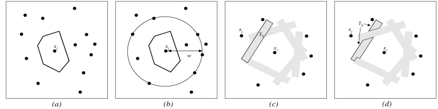
Figure 2. The Bounding Process. (a) A codeword $x_{i}$, neighboring codewords and the Voronoi region $D(x_{i})$. (b) We restrict our attention to only those neighbors that are a distance $w$ away. By only worrying that the received word $y$ is closer to this subset of the neighbors we upper bound $\mathbb{P}_{i}\left(D(x_{i})\right)$. (c) For each neighbor $x_{j}$ still under consideration, let $X_{ij}$ be some set of words that are closer to $x_{j}$ than they are to $x_{i}$. (d) We “prune” the $X_{ij}$’s to construct disjoint $Y_{ij}$’s with the required properties.

See Figure 2 for an illustration of the bounding process. To create the $Y_{ij}$’s from the $X_{ij}$’s we randomly “prune” these sets so that the disjointness condition is satisfied. To accomplish this pruning we define a set of codewords $T_{i}=\{x_{j}:d_{ij}=w\}$ for each codeword $x_{i}$. Then, as in [7], for each $x_{i}$, we randomly index by $s_{ij}$ all the codewords $x_{j}$ that are a distance $w$ from $x_{i}$. Define sets

$$T(i,j)=\{k\in T_{i}:s_{ik}<s_{ij}\}.$$

We then get our $Y_{ij}$’s as follows

$$Y_{ij}=X_{ij}\setminus[\cup_{k\in T(i,j)}X_{ik}].$$

These $Y_{ij}$ satisfy the disjointness condition: assume there exists $x\in Y_{im}\cap Y_{il}$. Then $x\in X_{im}$ and $x\not\in\bigcup_{k\in T(i,m)}X_{ik}$ gives that $s_{il}>s_{im}$. However we also have $x\in X_{il}$ and $x\not\in\bigcup_{k\in T(i,l)}X_{ik}$ and this gives that $s_{im}>s_{il}$ which is a contradiction.

Instead of calculating $\mathbb{P}_{i}\left(Y_{ij}\right)$ directly we apply a “reverse union bound” to get

(20) $$\mathbb{P}_{i}\left(Y_{ij}\right)\geq\mathbb{P}_{i}\left(X_{ij}\right)(1-K_{ij}),$$

where $K_{ij}=\sum_{k\in T(i,j)}\mathbb{P}_{i}\left(X_{ik}|X_{ij}\right)$. Note that this inequality is the bound (3) with our particular choice of $X_{ij},Y_{ij}.$ Using the last inequality we perform a recursive procedure which shows the existence of a subcode $C^{\prime}\subset C$ with large error probability (among the codewords of $C^{\prime}$). This gives the claimed lower bound on $P_{e}(C,p).$

2.3. A proof of Theorem 6

The error probability for two codewords is given by the following well-known lemma.

Lemma 8.

For all codewords $x_{i}$ and $x_{j}$ that are a distance $w$ apart $\lim_{n\to\infty}\frac{1}{n}\log P_{i}(X_{ij})=A(\omega),$ where $A(\omega)$ is defined in (1).

Lemma 9.

For all codewords $x_{i}$, $x_{j}$ and $x_{k}$ such that $d_{ij}=d_{ik}=w$ and $d_{jk}=l$ we have

$$\lim_{n\to\infty}\frac{1}{n}\log\mathbb{P}_{i}\left(X_{ik}|X_{ij}\right)=B(\omega,\lambda)$$

where $B(\omega,\lambda)$ is defined in Eq. (9).

Proof.

First consider

$$\mathbb{P}_{i}\left(X_{ik}\cap X_{ij}\right)= \sum_{m=0}^{\min(l/2,p(n-w))}\left(\negthickspace\begin{array}[]{c}l/2\\ m\end{array}\negthickspace\right)^{2}\times\left(\negthickspace\begin{array}[]{c}w-l/2\\ w/2-m\end{array}\negthickspace\right)\left(\negthickspace\begin{array}[]{c}n-w-l/2\\ p(n-w)-m\end{array}\negthickspace\right)$$

$$\times p^{w/2+p(n-w)}(1-p)^{n-w/2-p(n-w)}.$$

Then since

$$\log\mathbb{P}_{i}\left(X_{ik}|X_{ij}\right)=\log\mathbb{P}_{i}\left(X_{ik}\cap X_{ij}\right)-\log\mathbb{P}_{i}\left(X_{ij}\right),$$

substituting for $\mathbb{P}_{i}\left(X_{ij}\right)$ from the previous lemma and taking the appropriate limits gives the required result. ∎

The following properties of $B(\omega,\lambda)$ can be verified numerically.

Lemma 10.

If $\omega\leq\lambda\leq 2\omega$ then $B(\omega,\lambda)\leq B(\omega,\omega)$. If $\lambda\leq\omega$ then $B(\lambda,\lambda)\leq B(\omega,\lambda)$

Recall that the indexing of pairs to create the sets $T(i,j)$ is done randomly. By linearity of expectation there exists an indexing such that

(21) $$P_{e}\geq\frac{1}{M}\sum_{i=1}^{M}\sum_{j:d_{ij}=w}\mathbb{E}\left(\mathbb{P}_{i}\left(Y_{ij}\right)\right)$$

This equation will be the basis for our new bound on the error exponent but before deriving this bound we have two final preliminaries. Firstly we will refer to all codewords $x_{j}$ that are a distance $w$ from $x_{i}$ as $w$-neighbors of $x_{i}$. (Recall that we defined $B_{w}^{i}$ to be the number of codewords in the $w$-neighborhood of $x_{i}$.) Secondly we shall say that a subset $S^{\prime}\subseteq S$ of codewords is of substantial size (with respect to $S$) if its size has the same exponential order as the size of $S$. Note that for a family of codes $(C_{i})_{i\geq 1}$ where $C_{i}$ has length $n$ and rate $R$, we can consider $(C_{i}^{{}^{\prime}})_{i\geq 1}$, a family of codes where $C^{\prime}_{i}$ is a substantially sized subcode of $C_{i}$, when trying to bound the error exponent since

$$\lim_{n\to\infty}R(C^{\prime}_{i})=\lim_{n\to\infty}R(C_{i})=R$$

and

$$\limsup_{n\to\infty}\frac{1}{n}\log\frac{1}{P_{e}(C_{i}^{{}^{\prime}},p)}\geq\limsup_{n\to\infty}\frac{1}{n}\log\frac{1}{P_{e}(C_{i},p)}.$$

We now proceed with a case analysis dependent on the values of $K_{ij}$. Roughly speaking when $K_{ij}$ is typically less than a half, a union bound argument will be used to bound the error probability. When $K_{ij}$ is typically larger than a half, a more complicated analysis will be required. Before we describe the two cases in our analysis we need the following two lemmas.

Lemma 11.

[8] Suppose that there are $L$ balls of $K$ different colors. The number of balls of a color $k$ is $r_{k}$. We are also given numbers $n_{k},1\leq k\leq K$. Suppose that all balls are enumerated randomly by different integers from 1 up to $L$. Let $\tau$ be a random integer between 1 and $L$ and let $t_{k}$ be the number of balls of color $k$ with numbers between 1 and $\tau$. Then

$$\mathbb{P}\left(t_{k}\leq n_{k},k=1,\ldots K\right)\geq\min\Big{\{}1,\frac{1}{4}\min_{1\leq k\leq K}\frac{n_{k}}{r_{k}}\Big{\}}.$$

Recall that, for a given $(i,j)$ pair, $K_{ij}$ is a random variable. We then can prove the following lemma:

Lemma 12.

Let $d_{ij}=\omega n$. With respect to the random indexing of all the $(i,k)$ pairs (where $x_{k}$ is any codeword such that $d_{ik}=\omega n$) we have

$$\mathbb{P}\left(K_{ij}\leq\frac{1}{2}\right)\geq\min\Big{\{}1,\min_{l\in\Lambda}\frac{2^{-nB(\omega,\lambda)-o(n)}}{\min\{B_{w}^{i},B_{l}^{j}\}}\Big{\}}$$

where $\Lambda=\{l\in[n]:|R_{w,l}|>N_{w,l}\}$, $R_{w,l}=\{x_{k}\in C:d_{ij}=d_{ik}=w,d_{jk}=l\}$ and $N_{w,l}=\frac{2^{-nB(\omega,\lambda)}}{2(n+1)}$.

Proof.

$$\mathbb{P}(K_{ij} \leq 1/2)=\mathbb{P}\left(\sum_{k\in T(i,j)}\mathbb{P}_{i}\left(X_{ik}|X_{ij}\right)\leq 1/2\right)$$

$$\cong\mathbb{P}\left(\sum_{l=0}^{n}\sum_{k\in T(i,j),d_{jk}=l}2^{nB(\omega,\lambda)}\leq 1/2\right)$$

$$=\mathbb{P}\left(\sum_{l=0}^{n}|T(i,j)\cap R_{w,l}|2^{nB(\omega,\lambda)}\leq 1/2\right)$$

$$\geq\mathbb{P}\left(|T(i,j)\cap R_{w,l}|\leq N_{w,l}\;\forall l\in\Lambda\right).$$

Let there be a ball for each codeword in $\bigcup_{l}R_{w,l}.$ Consider a ball from $R_{w,l}$ to have color $l$. Let $n_{l}=N_{w,l}$ and $\mu_{l}=|x_{m}\in R_{w,l}:s_{im}<s_{ij}|.$ We have

$$\mathbb{P}\left(K_{ij}\leq 1/2\right)\geq\mathbb{P}\left(\mu_{l}\leq n_{l}\;\forall l\in\Lambda\right).$$

By the previous lemma we have

$$\mathbb{P}\left(\mu_{l}\leq n_{l}\;\forall l\in\Lambda\right)\geq\frac{1}{4}\min_{l\in\Lambda}\frac{n_{l}}{|R_{w,l}|}$$

if the right-hand side is less than one. The lemma then follows from the fact that $|R_{w,l}|\leq\min\{B_{w}^{i},B_{l}^{j}\}$. ∎

In the analysis that leads to Theorem 6, we face a dichotomy of a relatively sparse $w$-neighborhood of the transmitted vector $x_{i}$ when the union bound is asymptotically tight, and a cluttered neighborhood when is not. These two cases correspond to the first and the second terms in (17), respectively. When the union bound analysis is not applicable, we will rely crucially on the following lemma.

Lemma 13.

If $K_{ij}>1/2$ for some $i,j$ such that $d_{ij}=\omega n$ then there exists a nonempty set $\Lambda_{ij}$ such that for all $\lambda\in\Lambda_{ij}$,

$$\min\{B_{w}^{i},B_{\lambda n}^{j}\}>2^{-nB(\omega,\lambda)-o(n)}.$$

Proof.

Consider a pair of codewords $x_{i}$ and $x_{j}$ such that $K_{ij}>1/2$. We deduce that $\mathbb{P}\left(K_{ij}\leq 1/2\right)<1$ since the event $\{K_{ij}>1/2\}$ occurred. Therefore, by Lemma 12, there exists a $\lambda$ such that,

$$\frac{2^{-nB(\omega,\lambda)-o(n)}}{\min\{B_{w}^{i},B_{\lambda n}^{j}\}}<1.$$

∎

Given a pair of codewords $x_{i},x_{j}$ with $K_{ij}\leq 1/2$ we put $\Lambda_{ij}=\emptyset;$ otherwise, we assume that $\Lambda_{ij}$ contains all the values of $\lambda=l/n$ whose existence is established in the previous lemma. We now define, for all $n$ possible values of $l=\lambda n$, the sets

$$G_{l,w}=\{x_{j}:\exists x_{i}\mbox{ such that }K_{ij}>\nicefrac{{1}}{{2}}\text{ and }l/n\in\Lambda_{ij}\}.$$

In words, for a given $l$, the set $G_{l,w}\subset C$ contains all the codewords $x_{j}$ that have a $w$-neighbor $x_{i}$ such that the set $\Lambda_{ij}$ contains the value $\lambda=l/n.$ Let $H_{l,w}$ be defined as the set of all $x_{i}\in C$ such that a substantial number of the $w$-neighbors $x_{j}$ of $x_{i}$ satisfy $K_{ij}>\nicefrac{{1}}{{2}}$ and $l/n\in\Lambda_{ij}.$ Note that the “substantial number” here is in relation to $B^{i}_{w}$.

We say $\lambda=l/n$ is a “nuisance level” for $\omega$ if $H_{l,w}$ and $G_{l,w}$ are both substantially sized subcodes of $C$. The two cases in the following analysis correspond to whether or not a nuisance level exists. The next theorem bounds the error probability in the case that it does not exist.

Theorem 14.

Consider any code $C$ of sufficiently large length $n$ and rate $R$. Assume that for some $\omega$ and bounding function $f$ we have $\frac{1}{n}\log B_{\omega n}^{i}\geq f(\omega)$ for all $i$. If there does not exist a nuisance level for $\omega$ then

$$\frac{1}{n}\log\frac{1}{P_{e}(C,p)}\leq-f(\omega)-A(\omega)+o(1).$$

Proof.

Let us define the sets

$$S_{1}=\{l:H_{l,w}\mbox{ is not a substantially sized sub-code}\},$$

$$S_{2}=\{l:G_{l,w}\mbox{ is not a substantially sized sub-code}\}.$$

Since $w$ does not have a nuisance level, $S_{1}\cup S_{2}=[n]$. Without loss of generality we may assume that $G_{l,w}=\emptyset$ for all $l\in S_{2}$ since removing $\bigcup_{l\in S_{2}}G_{l,w}$ yields a substantially sized subcode. Hence also $H_{l,w}=\emptyset$ for all $l\in S_{2}$. Now consider only transmitting the codewords in $C^{\prime}=C\setminus\bigcup_{l\in[n]}H_{l,w}$ and note that this is a substantially sized number of codewords since neither $\bigcup_{l\in S_{1}}H_{l,w}$ nor $\bigcup_{l\in S_{2}}H_{l,w}$ are substantially sized. For each of these codewords we know that $\frac{1}{n}\log B_{\omega n}^{i}\geq f(\omega)$. Hence

$$P_{e}(C,p) \geq\frac{1}{M}\sum_{i=1}^{M}\sum_{j:d_{ij}=w}\mathbb{P}_{i}\left(Y_{ij}\right)$$

$$\gtrsim\frac{1}{M}\sum_{x_{i}\in C^{\prime}}B_{w}^{i}\min_{j:d_{ij}=w}\{\mathbb{P}_{i}\left(Y_{ij}\right)\}$$

$$\geq\frac{1}{2}\min_{i,j:d_{ij}=w}(B_{w}^{i}\mathbb{P}_{i}\left(X_{ij}\right))$$

$$\geq 2^{n(A(\omega)+f(\omega))-o(n)}.$$

The second inequality follows from the fact that for each $x_{i}\in C^{\prime}$, a substantial number of $w$-neighbors $x_{j}$ are such that $K_{ij}\leq 1/2$, and the third one is implied by (20) since $\mathbb{P}_{i}\left(Y_{ij}\right)\geq\mathbb{P}_{i}\left(X_{ij}\right)/2$ whenever $K_{ij}\leq 1/2$. ∎

We now bound the error probability (and ensure another property of the distance distribution) in the case that there exists a nuisance level.

Theorem 15.

Consider any code $C$ of sufficiently large length $n$ and rate $R$ and an $\omega\in[0,1]$. Let $\lambda$ be a nuisance level for $\omega.$ The subset of codewords $x_{j}\in C$ such that

$$|\{x_{k}\in C:\mathop{d}(x_{j},x_{k})=\lambda n\}|\geq 2^{-nB(\omega,\lambda)-o(n)}$$

forms a substantially sized subcode. Furthermore,

$$\frac{1}{n}\log\frac{1}{P_{e}(C,p)}\leq B(\omega,\lambda)-A(\omega)+o(1).$$

Proof.

Since $G_{l,w}$ is substantially sized, it follows by Lemma 13 that a substantial number of codewords $x_{j}$ have at least $2^{-nB(\omega,\lambda)-o(n)}$ neighbors at a relative distance $\lambda$. Now consider $x_{i}\in H_{l,w}.$ By definition, there is a substantially sized subset $N(i)$ of the $\omega n$-neighbors of $x_{i}$ such that $\lambda\in\Lambda_{ij}$ for all $x_{j}\in N(i)$. Hence, appealing to Lemma 12, for each $x_{j}\in N(i)$,

$$\mathbb{P}\left(K_{ij}\leq 1/2\right)\geq\frac{2^{-nB(\omega,\lambda)-o(n)}}{B_{w}^{i}}.$$

Now

$$\mathbb{E}\left(\mathbb{P}_{i}\left(Y_{ij}\right)\right) =\mathbb{E}\left(I_{K_{ij}\leq\frac{1}{2}}\mathbb{P}_{i}\left(Y_{ij}\right)\right)+\mathbb{E}\left(I_{K_{ij}>\frac{1}{2}}\mathbb{P}_{i}\left(Y_{ij}\right)\right)$$

$$\geq\mathbb{E}\left(I_{K_{ij}\leq\frac{1}{2}}\mathbb{P}_{i}\left(Y_{ij}\right)\right)$$

$$\geq\frac{2^{nA(\omega)}}{2}\mathbb{P}\left(K_{ij}\leq\frac{1}{2}\right),$$

and so, by the above discussion and Eq. (21), we get

$$P_{e} \geq\frac{1}{M}\sum_{x_{i}\in H_{l,w}}\sum_{j\in N(i)}\mathbb{E}\left(\mathbb{P}_{i}\left(Y_{ij}\right)\right)$$

$$\geq\frac{1}{M}\sum_{x_{i}\in H_{l,w}}2^{nA(\omega)}2^{-nB(\omega,\lambda)-o(n)}$$

$$=2^{n(A(\omega)-B(\omega,\lambda))-o(n)}.$$

∎

Proof of Theorem 6..

Let $C$ be the code from the statement of the theorem. Let

$$F=\frac{1}{n}\log\frac{1}{P_{e}(C,p)}.$$

As discussed in [2], [7], for any $w=\omega n,\delta\leq\omega\leq 1,$ the code $C$ contains a subcode $C^{\prime}$ of size $M^{\prime}\geq M/n^{2}$ such that for all codewords $x_{i}$ in this subcode

$$\frac{1}{n}\log B_{\omega n}^{i}>\beta(\omega)-o(n).$$

Since the subcode is substantially sized we may now consider this subcode as our new code.

For a fixed $\omega$ construct $Y_{ij},X_{ij}$ and $K_{ij}$ for all $(i,j)$ pairs with $d_{ij}=\omega n$. By Theorems 14 and 15 we get

$$F\leq\left\{\begin{array}[]{l@{\qquad}l}-\beta(\omega)-A(\omega)&\mbox{ if no nuisance level exists for $\omega$}\\ B(\omega,\lambda_{1})-A(\omega)&\mbox{ if a nuisance level $\lambda_{1}$ exists for $\omega$.}\\ \end{array}\right.$$

Hence we get

$$F\leq\max\{-\beta(\omega),B(\omega,\lambda_{1})\}-A(\omega).$$

Now if $\lambda_{1}\geq\omega$ then $B(\omega,\lambda_{1})\leq B(\omega,\omega)$ and so we get

(22) $$F\leq\max\{-\beta(\omega),B(\omega,\omega)\}-A(\omega).$$

If $\lambda_{1}<\omega$ then we use the fact from Theorem 15 that for a substantial number of codewords $x_{i}$, $B_{\lambda_{1}n}^{i}\geq 2^{-nB(\omega,\lambda_{1})}$. We now construct new $Y_{ij},X_{ij}$ and $K_{ij}$ for all $(i,j)$ pairs with $d_{ij}=\lambda_{1}n$. Hence by Theorems 14 and 15 we get

$$F\leq\left\{\begin{array}[]{l@{\qquad}l}B(\omega,\lambda_{1})-A(\lambda_{1})&\mbox{ if no nuisance level exists for $\lambda_{1}$}\\ B(\lambda_{1},\lambda_{2})-A(\lambda_{1})&\mbox{ if a nuisance level $\lambda_{2}$ exists for $\lambda_{1}$.}\end{array}\right.$$

Hence we get

$$F\leq\max\{B(\omega,\lambda_{1}),B(\lambda_{1},\lambda_{2})\}-A(\lambda_{1}).$$

If $\lambda_{2}\geq\lambda_{1}$ then $B(\lambda_{1},\lambda_{2})\leq B(\lambda_{1},\lambda_{1})\leq B(\omega,\lambda_{1})$ then

$$F\leq B(\omega,\lambda_{1})-A(\lambda_{1}).$$

If $\lambda_{2}<\lambda_{1}$ then we use the fact that for a substantial number of codewords $x_{i}$, $B_{\lambda_{2}n}^{i}\geq 2^{-nB(\lambda_{1},\lambda_{2})}$ and continue as before.

We continue in this manner and get a sequence $\omega>\lambda_{1}>\lambda_{2}\ldots$ such that at step $i$ we get the bound

$$F\leq\max\{B(\lambda_{i-1},\lambda_{i}),B(\lambda_{i},\lambda_{i+1})\}-A(\lambda_{i}).$$

This process terminates after at most $n$ steps since there are only $n$ possible values for the nuisance level. At the last step, $i=f$, the nuisance level $\lambda_{f+1}$, if it even exists, is not less than $\lambda_{f}$ itself and therefore we have

$$F \leq\max\{B(\lambda_{f-1},\lambda_{f}),B(\lambda_{f},\lambda_{f+1})\}-A(\lambda_{f})$$

$$\leq\max\{B(\lambda_{f-1},\lambda_{f}),B(\lambda_{f},\lambda_{f})\}-A(\lambda_{f})$$

$$\leq B(\omega,\lambda_{f})-A(\lambda_{f}).$$

Now for our code either this equation or Eq. (22) is valid, and so we have shown that for every $\omega,\delta\leq\omega\leq 1$ there exists $\lambda\leq\omega$ such that

$$F\leq\max(-\beta(\omega)-A(\omega),B(\omega,\lambda)-A(\lambda)).$$

This completes the proof. ∎

3. More on the bound of Theorem (7)

In this section we take a closer look at the bound (18) with the aim to show that it provides a new segment of code rates where the BSC channel reliability is known exactly. We rely on the notation of Sect. 1.1. Let $R_{x}=1-h(2\rho(1-\rho)).$ Recall that the best known lower bound on $E(R,p)$ below the critical rate is given by

(23) $$E_{x}(R,p)=-A(\delta_{\text{\rm GV}}(R))\quad 0\leq R\leq R_{x}$$

(24) $$E_{0}(R,p)=D(\rho\|p)+R_{\text{crit}}-R\quad R_{x}<R\leq R_{\text{crit}}.$$

For $R>R_{\text{crit}}$ the reliability function $E(R,p)=E_{\text{sp}}(R,p).$ Note that both $E_{x}$ and $E_{\text{sp}}(R,p)$ can be viewed as instances of the union bound and that both are tangent on $E_{0}(R,p).$ Let us make one simple observation showing that the bound (18) has the same property.

The following lemma is verified by direct calculation.

Lemma 16.

Let $\delta_{1}=2\rho(1-\rho)$ and let $R_{1}=\bar{R}(\delta_{1}).$ Then

$$-A(\delta_{1})-R_{1}+1-h(\delta_{1})=E_{0}(R_{1},p).$$

Proof.

Indeed, (24) can be rewritten as

$$E_{0}(R,p)=1-R+\log(1+2\sqrt{p(1-p)}).$$

The equality in the statement is equivalent to the relation

$$h(\delta_{1})+\delta_{1}\log 2\sqrt{p(1-p)}=\log(1+2\sqrt{p(1-p)})$$

which is an easily verifiable identity. ∎

Next we can prove the main result of this section.

Theorem 17.

Let $p,0.046\leq p<1/2$ be the channel transition probability. Then the channel reliability $E(R,p)$ equals the random coding exponent $E_{0}(R,p)$ for $R_{1}\leq R\leq R_{\text{crit}}.$

Proof.

We check numerically that $R_{1}<R_{0}^{\ast}$ for $p\geq 0.046.$ Thus, by Theorem 7 for these values of $p$ we have $E(R_{1},p)=E_{0}(R_{1},p).$ The full claim follows from the straight-line bound of Shannon, Gallager, and Berlekamp [27]. ∎

Remark. We have seen in Lemma 4 that for $p\geq 0.037,$ it suffices to rely on the simple form of the function $\bar{R}(x),$ namely $R(x)=\varphi(x)$. Thus the only numerical calculation involved in the proof of this theorem relates to the function $B(\omega,\delta).$

The random coding exponent $E_{0}(R,p)$ gives the best known lower bound on $E(R,p)$ for $R_{x}\leq R\leq R_{\text{crit}}.$ The fraction of this segment in which Theorem 17 shows it to be tight is given by

$$\frac{R_{\text{crit}}-R_{1}}{R_{\text{crit}}-R_{x}}.$$

This fraction equals about $1/3$ for $p=0.05$ and tends to one as $p\to\nicefrac{{1}}{{2}}.$

We give an example of the new picture for the $E(R,p)$ function in Fig. 3. Previously the reliability of the BSC was known exactly only for $R\geq R_{\text{crit}}$ [12].

Figure 3. Bounds on the error exponent for the BSC with $p=0.08$. In the interval $R_{1}\leq R\leq R_{\text{crit}}$ the random coding bound $E_{0}(R,p)$ is tight.

4. Random linear codes

The inequality of Theorem 6 can be used for a code with an arbitrary distance distribution. In this section we are interested in the estimate of the error exponent for a random linear code $C$. Here by a random code we mean a binary code whose weight distribution behaves as the binomial distribution: ${\mathcal{B}}_{\omega n}\cong\exp[n(R+h(\omega)-1)].$ The reason for calling this code random is that the weight distribution of a randomly chosen linear code with high probability converges to the binomial distribution (e.g. [3]).

The error exponent $\tilde{E}(R,p)$ for random linear codes for low rates is bounded below by the expurgation exponent: $\tilde{E}(R,p)\geq-A(\delta_{\text{\rm GV}}(R)).$ For $R_{x}\leq R_{0}\leq R_{\text{crit}},$ the exponent $\tilde{E}(R,p)\geq E_{0}(R,p).$ Moreover, it is known that the error probability $P_{e}(C)$ averaged over the ensemble of all binary codes meets this bound with equality [15]. The proof of this result in [15] is accomplished by computing the ensemble average probability of error under list decoding into lists of size 2, where by error we mean the event that the transmitted codeword is not in the resulting list. It turns out that under this definition the error occurs in an exponentially smaller fraction of cases than the error of maximum likelihood decoding. In other words, in all the cases of error under maximum likelihood decoding (i.e., decoding into a size-1 list) except for an exponentially small fraction of them, there is exactly one codeword which is at least as close to the received word as is the transmitted word. This shows that for exponential asymptotics of the error probability of random codes the union bound is tight. An analogous result can also be proved for the ensemble of binary linear codes.

Here we compute a lower bound on the decoding error probability of a code with weight distribution ${\mathcal{B}}_{\omega n}.$ A closed-form expression again seems beyond reach, however computational evidence with the bound (17) suggests that in a certain segment of code rates $0\leq R\leq R^{\ast\ast}$, the error exponent of maximum likelihood decoding of the code $C$ is bounded above as follows

$$\tilde{E}(R,p)\leq-A(\delta_{\text{\rm GV}}(R)).$$

In other words, the expurgation exponent is tight for a random linear code in the region of low code rates.

5. The Gaussian channel

Given the results for the BSC of Section 3, it is natural to assume that qualitatively similar results hold for the reliability function of the Gaussian channel. Here we consider briefly this problem and show that the random coding exponent is tight for a certain interval of rates immediately below the critical rate. As in the binary case, the length of this segment depends on the level of the channel noise.

Let $a$ be the signal-to-noise ratio in the channel. Denote by $E(R,a)$ the channel reliability function defined analogously to the BSC case. It is known to be bounded below by the random coding bound $E_{0}(R,a)$ [26] which has the form

$$E_{0}(R,a)=\frac{a}{4}(1-\cos\theta_{x})+R_{x}-R$$

and is the best known lower bound for $R_{x}\leq R\leq R_{\text{crit}}$ where

$$R_{x}=\frac{1}{2}\ln\Big{(}\frac{1}{2}+\frac{1}{2}\sqrt{1+\frac{a^{2}}{4}}\,\Big{)},$$

$$\theta_{x}=\cos^{-1}\sqrt{1-e^{-2R_{x}}},$$

$$R_{\text{crit}}=\frac{1}{2}\ln\Big{(}\frac{1}{2}+\frac{a}{4}+\frac{1}{2}\sqrt{1+\frac{a^{2}}{4}}\,\Big{)}.$$

Let $C$ be a code on $S^{n-1}({\mathbb{R}})$ (the unit sphere in ${\mathbb{R}}^{n}$). Let $\theta(x_{i},x_{j})$ be the angle between the vectors that correspond to the codewords $x_{i},x_{j}$. Denote by $B(\theta)$ the distribution of angular distances in the code $C$. The exponent of the union bound on the error probability $P_{e}(C,a)$ has the form

$$E_{U}=\frac{a}{4}(1-\cos\theta)-\frac{1}{n}\ln B(\theta).$$

Used together with an estimate of the distance distribution of a code of rate $R$ obtained in [2] this bound takes the form

$$E_{U}(R,a)=\frac{a}{4}(1-\cos\bar{\theta})-\ln\sin\bar{\theta}-R,$$

where $\bar{\theta}=\bar{\theta}(R)$ is the root of the equation $R=\psi(\theta)$ and

$$\psi(x)=-\frac{1-\sin x}{2\sin x}\ln\frac{1-\sin x}{1+\sin x}-\ln\frac{2\sin x}{1+\sin x}$$

(which represents the Kabatiansky-Levenshtein bound on spherical codes). The strongest known condition for the union bound to be valid asymptotically as a lower bound on $P_{e}(C,a)$ was announced in [5]. According to it, $E(R,a)\leq E_{U}(R,a)$ for all rates $R\leq R^{\ast}$, where $R^{\ast}$ is the root of

(25) $$R+\ln\sin\bar{\theta}(R)=\frac{a}{8}(1-\cos\bar{\theta}).$$

Other conditions were obtained in [2, 7, 9].

Next we state a result analogous to Lemma 16. Its proof is immediate by comparing the expressions for $E_{U}$ and $E_{0}.$

Lemma 18.

Let $R_{1}=\psi(\theta_{x}),$ then $E_{0}(R_{1},a)=E_{U}(R_{1},a).$

We conclude that $E_{0}(R_{1},a)$ is the correct value of $E(R_{1},a)$ if $R_{1}\leq R^{\ast}.$ The last inequality holds for $0<a\leq 5.7.$ Coupled with the straight-line principle of [27] this gives

Theorem 19.

Let $0<a\leq 5.7$ be the signal-to-noise ratio in the channel. Then

$$E(R,a)=E_{0}(R,a)\qquad(R_{1}\leq R\leq R_{c}).$$

Example. For instance, let $a=2$. Then $R_{x}=0.094,R_{1}=0.199,R^{\ast}=0.263,R_{\text{crit}}=0.267$.

If instead of (25) we rely on conditions with a published proof, we would still be able to make a tightness claim of $E_{0}$ but for a smaller segment of the signal-to-noise ratio values.

Postscriptum: Recently, a generalized de Caen inequality was used to derive lower estimates of error probability of a code via its distance distribution [9]. In particular, [9] gives a condition for the union bound to be valid asymptotically as a lower bound on $P_{e}$ in the BSC case. Although the condition is stated as an optimization problem ([9], Prop. 5.3), computational evidence suggests that its solution is given by (16). Thus, the methods of this paper and of [9], although different in nature, seem to lead to the same general estimates. Note that [9] does not contain results on the BSC reliability function.

References

- [1] A. Ashikhmin and A. Barg, Binomial moments of the distance distribution: Bounds and applications, IEEE Trans. Inform. Theory 45 (1999), no. 2, 438–452.
- [2] A. Ashikhmin, A. Barg, and S. Litsyn, A new upper bound on the reliability function of the Gaussian channel, IEEE Trans. Inform. Theory 46 (2000), no. 6, 1945–1961.
- [3] A. Barg and G. D. Forney, Jr., Random codes: Minimum distances and error exponents, IEEE Trans. Inform. Theory 48 (2002), no. 9, 2568–2573.
- [4] R. E. Blahut, Principles and practice of information theory, Addison-Wesley, Reading, MA, 1987.
- [5] M. V. Burnashev, On relation between code geometry and decoding error probability, Proc. 2001 IEEE Internat. Sympos. Inform. Theory, Washington, DC, p.133.
- [6] by same author, A new lower bound for the -mean error of parameter transmission over the white Gaussian channel, IEEE Trans. Inform. Theory 30 (1984), no. 1, 23–34.
- [7] by same author, On the relation between the code spectrum and the decoding error probability, Problems of Information Transmission 36 (2000), no. 4, 3–24.
- [8] M. V. Burnashev and Y. A. Kutoyants, On minimal -mean error parameter transmission over a Poisson channel, IEEE Trans. Inform. Theory 47 (2001), no. 6, 2505–2515.
- [9] A. Cohen and N. Merhav, Lower bounds on the error probability of block codes based on improvements of de Caen’s inequality, IEEE Trans. Inform. Theory (2004), no. 2, 290–310.
- [10] I. Csiszár and J. Körner, Information theory. Coding theorems for discrete memoryless channels, Akadémiai Kiadó, Budapest, 1981.
- [11] D. de Caen, A lower bound on the probability of a union, Discrete Math. 169 (1997), no. 1-3, 217–220.
- [12] P. Elias, Coding for noisy channels, IRE Conv. Rec., Mar. 1955, pp. 37–46. Reprinted in D. Slepian, Ed., Key papers in the development of information theory, IEEE Press, 1974, pp. 102–111.
- [13] R. G. Gallager, Low-density parity-check codes, MIT Press, Cambridge, MA, 1963.
- [14] by same author, Information theory and reliable communication, John Wiley & Sons, New York e.a., 1968.
- [15] by same author, The random coding bound is tight for the average code, IEEE Trans. Inform. Theory (1973), no. 2, 244–246.
- [16] G. Kalai and N. Linial, On the distance distribution of codes, IEEE Trans. Inform. Theory 41 (1995), no. 5, pp. 1467-1472.
- [17] O. Keren and S. Litsyn, A lower bound on the probability of error on a bsc channel, The 21st IEEE Convention of the Electrical and Electronic Engineers in Israel, 2000, pp. 217–220.
- [18] E. G. Kounias, Bounds for the probability of a union, with applications, Ann. Math. Statist. 39 (1968), 2154–2158.
- [19] H. Kuai, F. Alajaji, and G. Takahara, A lower bound on the probability of a finite union of events, Discrete Math. 215 (2000), no. 1-3, 147–158.
- [20] by same author, Tight error bounds for nonuniform signalling over AWGN channels, IEEE Trans. Inform. Theory 46 (2000), no. 7, 2712–2718.
- [21] S. Litsyn, New upper bounds on error exponents, IEEE Trans. Inform. Theory 45 (1999), no. 2, 385–398.
- [22] R. J. McEliece and J. K. Omura, An improved upper bound on the block coding error exponent for binary-input discrete memoryless channels, IEEE Trans. Inform. Theory 23 (1977), no. 5, 611–613.
- [23] R. J. McEliece, E. R. Rodemich, H. Rumsey, and L. R. Welch, New upper bound on the rate of a code via the Delsarte-MacWilliams inequalities, IEEE Trans. Inform. Theory 23 (1977), no. 2, 157–166.
- [24] G. Sh. Poltyrev, Bounds on the decoding error probability of binary linear codes via their spectra, IEEE Trans. Inform. Theory 40 (1994), no. 4, 1284–1292.
- [25] G. E. Séguin, A lower bound on the error probability for signals in white Gaussian noise, IEEE Trans. Inform. Theory 44 (1998), no. 7, 3168–3175.
- [26] C. E. Shannon, Probability of error for optimal codes in a Gaussian channel, Bell Syst. Techn. Journ. 38 (1959), no. 3, 611–656.
- [27] C. E. Shannon, R. G. Gallager, and E. R. Berlekamp, Lower bounds to error probability for codes on discrete memoryless channels, II, Information and Control 10 (1967), 522–552.
- [28] A. J. Viterbi and J. K. Omura, Principles of digital communication and coding, McGraw-Hill, 1979.