Predicate Abstraction with Indexed Predicates

Abstract

Predicate abstraction provides a powerful tool for verifying properties of infinite-state systems using a combination of a decision procedure for a subset of first-order logic and symbolic methods originally developed for finite-state model checking. We consider models containing first-order state variables, where the system state includes mutable functions and predicates. Such a model can describe systems containing arbitrarily large memories, buffers, and arrays of identical processes. We describe a form of predicate abstraction that constructs a formula over a set of universally quantified variables to describe invariant properties of the first-order state variables. We provide a formal justification of the soundness of our approach and describe how it has been used to verify several hardware and software designs, including a directory-based cache coherence protocol.

A shorter version of the paper appeared at International Conference on Verification, Model Checking and Abstract Interpretation, (VMCAI) 2004

1 Introduction

Graf and Saïdi introduced predicate abstraction [Graf and Saidi (1997)] as a means of automatically determining invariant properties of infinite-state systems. With this approach, the user provides a set of $k$ Boolean formulas describing possible properties of the system state. These predicates are used to generate a finite state abstraction (containing at most $2^{k}$ states) of the system. By performing a reachability analysis of this finite-state model, a predicate abstraction tool can generate the strongest possible invariant for the system expressible in terms of this set of predicates. Prior implementations of predicate abstraction [Graf and Saidi (1997), Saidi and Shankar (1999), Das et al. (1999), Das and Dill (2001), Ball et al. (2001), Flanagan and Qadeer (2002), Chaki et al. (2003)] required making a large number of calls to a theorem prover or first-order decision procedure, and hence could only be applied to cases where the number of predicates was small. More recently, we have shown that both BDD and SAT-based Boolean methods can be applied to perform the analysis efficiently [Lahiri et al. (2003)].

In most formulations of predicate abstraction, the predicates contain no free variables, and hence they evaluate to true or false for each system state. The abstraction function $\alpha$ has a simple form, mapping each concrete system state to a single abstract state based on the effect of evaluating the $k$ predicates. The task of predicate abstraction is to construct a formula $\psi^{*}$ consisting of some Boolean combination of the predicates such that $\psi^{*}(s)$ holds for every reachable system state $s$.

To verify systems containing unbounded resources, such as buffers and memories of arbitrary size and systems with arbitrary numbers of identical, concurrent processes, the system model must support first-order state variables, in which the state variables are themselves functions or predicates [Ip and Dill (1996), Bryant et al. (2002b)]. For example, a memory can be represented as a function mapping an address to the data stored at an address, while a buffer can be represented as a function mapping an integer index to the value stored at the specified buffer position. The state elements of a set of identical processes can be modeled as functions mapping an integer process identifier to the state element for the specified process. In many systems, this capability is restricted to arrays that can be altered only by writing to a single location [Burch and Dill (1994), McMillan (1998)]. Our verifier allows a more general form of mutable function, where the updating operation is expressed using lambda notation.

In verifying systems with first-order state variables, we require quantified predicates to describe global properties of state variables, such as “At most one process is in its critical section,” as expressed by the formula $\forall i,j:\mathtt{crit}(i)\land\mathtt{crit}(j)\Rightarrow i=j$. Conventional predicate abstraction restricts the scope of a quantifier to within an individual predicate. System invariants often involve complex formulas with widely scoped quantifiers. The scoping restriction (the fact that the universal quantifier does not distribute over conjunctions) implies that these invariants cannot be divided into small, simple predicates. This puts a heavy burden on the user to supply predicates that encode intricate sets of properties about the system. Recent work attempts to discover quantified predicates automatically [Das and Dill (2002)], but this is a formidable task.

In this paper we present an extension of predicate abstraction in which the predicates include free variables from a set of index variables ${\cal X}$ (and hence the name indexed predicates). The predicate abstraction engine constructs a formula $\psi^{*}$ consisting of a Boolean combination of these predicates, such that the formula $\forall{\cal X}\psi^{*}(s)$ holds for every reachable system state $s$. With this method, the predicates can be very simple, with the predicate abstraction tool constructing complex, quantified invariant formulas. For example, the property that at most one process can be in its critical section could be derived by supplying predicates $\mathtt{crit}(\mathtt{i})$, $\mathtt{crit}(\mathtt{j})$, and $\mathtt{i}=\mathtt{j}$, where $\mathtt{i}$ and $\mathtt{j}$ are the index symbols. Encoding these predicates in the abstract system with Boolean variables $\mathtt{ci}$, $\mathtt{cj}$, and $\mathtt{eij}$, respectively, we can verify this property by using predicate abstraction to prove that $\mathtt{ci}\land\mathtt{cj}\Rightarrow\mathtt{eij}$ holds for every reachable state of the abstract system.

Flanagan and Qadeer use a method similar to ours [Flanagan and Qadeer (2002)], and we briefly described our method in an earlier paper [Lahiri et al. (2003)]. Our contribution in this paper is to describe the method more carefully, explore its properties, and to provide a formal argument for its soundness. The key idea of our approach is to formulate the abstraction function $\alpha$ to map a concrete system state $s$ to the set of all possible valuations of the predicates, considering the set of possible values for the index variables ${\cal X}$. The resulting abstract system is unusual; it is not characterized by a state transition relation and hence cannot be viewed as a state transition system. Nonetheless, it provides an abstraction interpretation of the concrete system [Cousot and Cousot (1977)] and hence can be used to find invariant system properties.

Assuming a decision procedure that can determine the satisfiability of a formula with universal quantifiers, we prove the following completeness result: Predicate abstraction can prove any property that can be proved by induction on the state sequence using an induction hypothesis expressed as a universally quantified formula over the given set of predicates. For many modeling logics, this decision problem is undecidable. By using quantifier instantiation, we can implement a sound, but incomplete verifier. As an extension, we show that it is easy to incorporate axioms into the system, properties that must hold universally for every system state. Axioms can be viewed simply as indexed predicates that must evaluate to true on every step.

The ideas have been implemented in UCLID [Bryant et al. (2002b)], a platform for modeling and verifying infinite-state systems. Although we demonstrate the ideas in the context of this tool and the logic (CLU) it supports, the ideas developed here are not strongly tied to this logic. We conclude the paper by describing our use of predicate abstraction to verify several hardware and software systems, including a directory-based cache coherence protocol devised by Steven German [(24)]. We believe we are the first to verify the protocol for a system with an unbounded number of clients, each communicating via unbounded FIFO channels.

1.1 Related Work

Verifying systems with unbounded resources is in general undecidable. For instance, the problem of verifying if a system of $N$ ($N$ can be arbitrarily large) concurrent processes satisfies a property is undecidable [Apt and Kozen (1986)]. Despite its complexity, the problem of verifying systems with arbitrary large resources (e.g. parameterized systems with $N$ processes, out-of-order processors with arbitrary large reorder buffers, software programs with arbitrary large arrays) is of significant practical interest. Hence, in recent years, there has been a lot of interest in developing techniques based on model checking and deductive approaches for verifying such systems.

McMillan uses “compositional model checking” [McMillan (1998)] with various built-in abstractions to reduce an infinite-state system to a finite state system, which can be model checked using Boolean methods. The abstraction mechanisms include temporal case splitting, datatype reduction [Clarke et al. (1992)] and symmetry reduction. Temporal case splitting uses heuristics to slice the program space to only consider the resources necessary for proving a property. Datatype reduction uses abstract interpretation [Cousot and Cousot (1977)] to abstract unbounded data and operations over them to operations over finite domains. For such finite domains, datatype reduction is subsumed by predicate abstraction. Symmetry is exploited to reduce the number of indices to consider for verifying unbounded arrays or network of processes. The method can prove both safety and liveness properties. Since the abstraction mechanisms are built into the system, they can often be coarse and may not suffice for proving a system. Besides, the user is often required to provide auxiliary lemmas or to decompose the proof to be discharged by symbolic model checkers. For instance, the proof of safety of the Bakery protocol [McMillan et al. (2000)] or the proof of an out-of-order processor model [McMillan (1998)] required non-trivial lemmas in the compositional model checking framework.

Regular model checking [Kesten et al. (1997), Bouajjani et al. (2000)] uses regular languages to represent parameterized systems and computes the closure for the regular relations to construct the reachable state space. In general, the method is not guaranteed to be complete and requires various acceleration techniques (sometimes guided by the user) to ensure termination. Moreover, approaches based on regular language are not suited for representing data in the system. Several examples that we consider in this work can’t be modeled in this framework; the out-of-order processor which contains data operations or the Peterson’s mutual exclusion are few such examples. Even though the Bakery algorithm can be verified in this framework, it requires considerable user ingenuity to encode the protocol in a regular language.

Several researchers have investigated restrictions on the system description to make the parameterized verification problem decidable. Notable among them is the early work by German and Sistla [German and Sistla (1992)] for verifying single-indexed properties for synchronously communicating systems. For restricted systems, finite “cut-off” based approaches [Emerson and Namjoshi (1995), Emerson and Kahlon (2000), Emerson and Kahlon (2003)] reduce the problem to verifying networks of some fixed finite size. These bounds have been established for verifying restricted classes of ring networks and cache coherence protocols. Emerson and Kahlon [Emerson and Kahlon (2003)] have verified the version of German’s cache coherence protocol with single entry channels by manually reducing it to a snoopy protocol, for which finite cut-off exists. However, the reduction is manually performed and exploits details of operation of the protocol, and thus requires user ingenuity. It can’t be easily extended to verify other unbounded systems including the Bakery algorithm or the out-of-order processors.

The method of “invisible invariants” [Pnueli et al. (2001), Arons et al. (2001)] uses heuristics for constructing universally quantified invariants for parameterized systems automatically. The method computes the set of reachable states for finite (and small) instances of the parameters and then generalizes them to parameterized systems to construct a potential inductive invariant. They provide an algorithm for checking the verification conditions for a restricted class of system called the stratified systems, which include German’s protocol with single entry channels and Lamport’s Bakery protocol [Lamport (1974)]. However, the method simply becomes a heuristic for generating candidate invariants for non-stratified systems, which includes Peterson’s mutual exclusion algorithm [Peterson (1981)] and the Ad-hoc On-demand Distance Vector (AODV) [C.Perkins et al. (2002)] network protocol. The class of bounded-data systems (where each variable is finite but parameterized) considered by this approach can’t model the the out-of-order processor model [Lahiri et al. (2002)] that we can verify using our method.

Predicate abstraction with locally quantified predicates [Das and Dill (2002), Baukus et al. (2002)] require complex quantified predicates to construct the inductive assertions, as mentioned in the introduction. These predicates are often as complex as invariants themselves. In fact, some of the invariants are used are predicates in [Baukus et al. (2002)] to derive inductive invariants. The method in [Baukus et al. (2002)] verified (both safety and liveness) a version of the cache coherence protocol with single entry channels, with complex manually provided predicates. Baukus et al. [Baukus et al. (2002)] uses the the logic of WSIS (weak second order logic with one successor) [Büchi (1960), Thomas (1990)], which does not allow function symbols and thus can’t model the out-of-order processor model. The automatic predicate discovery methods for quantified predicates [Das and Dill (2002)] have not been demonstrated on most examples (except the AODV model) we consider in this paper.

Flanagan and Qadeer [Flanagan and Qadeer (2002)] use indexed predicates to synthesize loop invariants for sequential software programs that involve unbounded arrays. They also provide heuristics to extract some of the predicates from the program text automatically. The heuristics are specific to loops in sequential software and not suited for verifying more general unbounded systems that we handle in this paper. In this work, we explore formal properties of this formulation and apply it for verifying distributed systems. In a recent work [Lahiri and Bryant (2004)], we provide a weakest precondition transformer [Dijkstra (1975)] based syntactic heuristic for discovering most of the predicates for many of the systems that we consider in this paper.

2 Notation

Rather than using the common indexed vector notation to represent collections of values (e.g., $\vec{v}\doteq\langle v_{1},v_{2},\ldots,v_{n}\rangle$), we use a named set notation. That is, for a set of symbols ${\cal A}$, we let $v$ indicate a set consisting of a value $v_{\mathtt{x}}$ for each $\mathtt{x}\in{\cal A}$.

For a set of symbols ${\cal A}$, let $\sigma_{\mbox{}\!{\cal A}}$ denote an interpretation of these symbols, assigning to each symbol $\mathtt{x}\in{\cal A}$ a value $\sigma_{\mbox{}\!{\cal A}}(\mathtt{x})$ of the appropriate type (Boolean, integer, function, or predicate). Let $\Sigma_{{\cal A}}$ denote the set of all interpretations $\sigma_{\mbox{}\!{\cal A}}$ over the symbol set ${\cal A}$.

For interpretations $\sigma_{\mbox{}\!{\cal A}}$ and $\sigma_{\mbox{}\!{\cal B}}$ over disjoint symbol sets ${\cal A}$ and ${\cal B}$, let $\sigma_{\mbox{}\!{\cal A}}\cdot\sigma_{\mbox{}\!{\cal B}}$ denote an interpretation assigning either $\sigma_{\mbox{}\!{\cal A}}(\mathtt{x})$ or $\sigma_{\mbox{}\!{\cal B}}(\mathtt{x})$ to each symbol $\mathtt{x}\in{\cal A}\cup{\cal B}$, according to whether $\mathtt{x}\in{\cal A}$ or $\mathtt{x}\in{\cal B}$.

Figure 1 displays the syntax of the Logic of Counter arithmetic with Lambda expressions and Uninterpreted functions (CLU), a fragment of first-order logic extended with equality, inequality, and counters. An expression in CLU can evaluate to truth values (bool-expr), integers (int-expr), functions (function-expr) or predicates (predicate-expr). Notice that we only allow restricted arithmetic on terms, namely that of addition or subtraction by constants. Notice that we restrict the parameters to a lambda expression to be integers, and not function or predicate expressions. There is no way in our logic to express any form of iteration or recursion.

bool-expr $$\mathrel{::=} {\bf true}\mathbin{|}{\bf false}\mathbin{|}\mbox{{\rm{\it bool-symbol}}}$$

$$|\;\neg\mbox{{\rm{\it bool-expr}}}\mathbin{|}(\mbox{{\rm{\it bool-expr}}}\land\mbox{{\rm{\it bool-expr}}})$$

$$|\;(\mbox{{\rm{\it int-expr}}}\!=\!\mbox{{\rm{\it int-expr}}})\mathbin{|}(\mbox{{\rm{\it int-expr}}}\!<\!\mbox{{\rm{\it int-expr}}})$$

$$|\;\mbox{{\rm{\it predicate-expr}}}(\mbox{{\rm{\it int-expr}}},\ldots,\mbox{{\rm{\it int-expr}}})$$

int-expr $$\mathrel{::=} \mbox{{\rm{\it lambda-var}}}\mathbin{|}\mbox{{\rm{\it int-symbol}}}$$

$$|\;\mbox{{\rm{\it ITE}}}(\mbox{{\rm{\it bool-expr}}},\,\mbox{{\rm{\it int-expr}}},\,\mbox{{\rm{\it int-expr}}})$$

$$|\;\mbox{{\rm{\it int-expr}}}+\mbox{{\rm{\it int-constant}}}$$

$$|\;\mbox{{\rm{\it function-expr}}}(\mbox{{\rm{\it int-expr}}},\ldots,\mbox{{\rm{\it int-expr}}})$$

predicate-expr $$\mathrel{::=} \mbox{{\rm{\it predicate-symbol}}}\mathbin{|}\lambda\,\mbox{{\rm{\it lambda-var}}},\ldots,\mbox{{\rm{\it lambda-var}}}\mathbin{.}\mbox{{\rm{\it bool-expr}}}$$

function-expr $$\mathrel{::=} \mbox{{\rm{\it function-symbol}}}\mathbin{|}\lambda\,\mbox{{\rm{\it lambda-var}}},\ldots,\mbox{{\rm{\it lambda-var}}}\mathbin{.}\mbox{{\rm{\it int-expr}}}$$

Figure 1: CLU Expression Syntax. Expressions can denote computations of Boolean values, integers, or functions yielding Boolean values or integers.

For symbol set ${\cal A}$, let $E({\cal A})$ denote the set of all CLU expressions over ${\cal A}$. For any expression $\phi\in E({\cal A})$ and interpretation $\sigma_{\mbox{}\!{\cal A}}\in\Sigma_{{\cal A}}$, let the valuation of $\phi$ with respect to $\sigma_{\mbox{}\!{\cal A}}$, denoted $\left\langle\phi\right\rangle_{\sigma_{\mbox{}\!{\cal A}}}$ be the (Boolean, integer, function, or predicate) value obtained by evaluating $\phi$ when each symbol $\mathtt{x}\in{\cal A}$ is replaced by its interpretation $\sigma_{\mbox{}\!{\cal A}}(\mathtt{x})$.

Let ${v}$ be a named set over symbols ${\cal A}$, consisting of expressions over symbol set ${\cal B}$. That is, $v_{\mathtt{x}}\in E({\cal B})$ for each $\mathtt{x}\in{\cal A}$. Given an interpretation $\sigma_{\mbox{}\!{\cal B}}$ of the symbols in ${\cal B}$, evaluating the expressions in ${v}$ defines an interpretation of the symbols in ${\cal A}$, which we denote $\left\langle{v}\right\rangle_{\sigma_{\mbox{}\!{\cal B}}}$. That is, $\left\langle{v}\right\rangle_{\sigma_{\mbox{}\!{\cal B}}}$ is an interpretation $\sigma_{\mbox{}\!{\cal A}}$ such that $\sigma_{\mbox{}\!{\cal A}}(\mathtt{x})=\left\langle v_{\mathtt{x}}\right\rangle_{\sigma_{\mbox{}\!{\cal B}}}$ for each $\mathtt{x}\in{\cal A}$.

A substitution $\pi$ for a set of symbols ${\cal A}$ is a named set of expressions over some set of symbols ${\cal B}$ (with no restriction on the relation between ${\cal A}$ and ${\cal B}$.) That is, for each $\mathtt{x}\in{\cal A}$, there is an expression $\pi_{\mathtt{x}}\in E({\cal B})$. For an expression $\psi\in E({\cal A}\cup{\cal C})$, we let $\psi\left[\pi/{\cal A}\right]$ denote the expression $\psi^{\prime}\in E({\cal B}\cup{\cal C})$ resulting when we replace each occurrence of each symbol $\mathtt{x}\in{\cal A}$ with the expression $\pi_{\mathtt{x}}$. These replacements are all performed simultaneously.

Proposition 2.1

Let $\psi$ be an expression in $E({\cal A}\cup{\cal C})$ and $\pi$ be a substitution having $\pi_{\mathtt{x}}\in E({\cal B})$ for each $\mathtt{x}\in{\cal A}$. For interpretations $\sigma_{\mbox{}\!{\cal B}}$ and $\sigma_{\mbox{}\!{\cal C}}$, if we let $\sigma_{\mbox{}\!{\cal A}}$ be the interpretation defined as $\sigma_{\mbox{}\!{\cal A}}=\left\langle\pi\right\rangle_{\sigma_{\mbox{}\!{\cal B}}}$, then $\left\langle\psi\right\rangle_{\sigma_{\mbox{}\!{\cal A}}\cdot\sigma_{\mbox{}\!{\cal C}}}=\left\langle\psi\left[\pi/{\cal A}\right]\right\rangle_{\sigma_{\mbox{}\!{\cal B}}\cdot\sigma_{\mbox{}\!{\cal C}}}$.

This proposition captures a fundamental relation between syntactic substitution and expression evaluation, sometimes referred to as referential transparency. We can interchangeably use a subexpression $\pi_{\mathtt{x}}$ or the result of evaluating this subexpression $\sigma_{\mbox{}\!{\cal A}}(\mathtt{x})$ in evaluating a formula containing this subexpression.

3 System Model

We model the system as having a number of state elements, where each state element may be a Boolean or integer value, or a function or predicate. We use symbolic names to represent the different state elements giving the set of state symbols ${\cal V}$. We introduce a set of initial state symbols ${\cal J}$ and a set of input symbols ${\cal I}$ representing, respectively, initial values and inputs that can be set to arbitrary values on each step of operation. Among the state variables, there can be immutable values expressing the behavior of functional units, such as ALUs, and system parameters such as the total number of processes or the maximum size of a buffer. Since these values are expressed symbolically, one run of the verifier can prove the correctness of the system for arbitrary functionalities, process counts, and buffer capacities.

The overall system operation is characterized by an initial-state expression set $q^{0}$ and a next-state expression set $\delta$. The initial state consists of an expression for each state element, with the initial value of state element $\mathtt{x}$ given by expression $q^{0}_{\mathtt{x}}\in E({\cal J})$. The transition behavior also consists of an expression for each state element, with the behavior for state element $\mathtt{x}$ given by expression $\delta_{\mathtt{x}}\in E({\cal V}\cup{\cal I})$. In this expression, the state element symbols represent the current system state and the input symbols represent the current values of the inputs. The expression gives the new value for that state element.

We will use a very simple system as a running example throughout this presentation. The only state element is a function $\mathtt{F}$, i.e. ${\cal V}$ = {$\mathtt{F}$}. An input symbol $\mathtt{i}$ determines which element of $\mathtt{F}$ is updated. Initially, $\mathtt{F}$ is the identify function:

$$q^{0}_{\mathtt{F}}=\lambda\,u\mathbin{.}u.$$

On each step, the value of the function for argument $\mathtt{i}$ is updated to be $\mathtt{F}(\mathtt{i}\!+\!1)$. That is,

$$\delta_{\mathtt{F}}=\lambda\,u\mathbin{.}\mbox{{\rm{\it ITE}}}(u=\mathtt{i},\,\mathtt{F}(\mathtt{i}\!+\!1),\,\mathtt{F}(u))$$

where the if-then-else operation ITE selects its second argument when the first one evaluates to true and the third otherwise. For the above example, ${\cal J}=\{\}$ and ${\cal I}$ = {$\mathtt{i}$}.

3.1 Concrete System

A concrete system state assigns an interpretation to every state symbol. The set of states of the concrete system is given by $\Sigma_{{\cal V}}$, the set of interpretations of the state element symbols. For convenience, we denote concrete states using letters $s$ and $t$ rather than the more formal $\sigma_{\mbox{}\!{\cal V}}$.

From our system model, we can characterize the behavior of the concrete system in terms of an initial state set $Q^{0}_{C}\subseteq\Sigma_{{\cal V}}$ and a next-state function operating on sets $N_{C}\colon{\mathscr{P}}({\Sigma_{{\cal V}}})\rightarrow{\mathscr{P}}({\Sigma_{{\cal V}}})$. The initial state set is defined as:

$$Q^{0}_{C}\doteq\{\left\langle q^{0}\right\rangle_{\sigma_{\mbox{}\!{\cal J}}}|\sigma_{\mbox{}\!{\cal J}}\in\Sigma_{{\cal J}}\},$$

i.e., the set of all possible valuations of the initial state expressions. The next-state function $N_{C}$ is defined for a single state $s$ as:

$$N_{C}(s)\doteq\{\left\langle\delta\right\rangle_{s\cdot\sigma_{\mbox{}\!{\cal I}}}|\sigma_{\mbox{}\!{\cal I}}\in\Sigma_{{\cal I}}\},$$

i.e., the set of all valuations of the next-state expressions for concrete state $s$ and arbitrary input. The function is then extended to sets of states by defining

$$N_{C}(S_{C})=\bigcup_{s\in S_{C}}N_{C}(s).$$

We can also characterize the next-state behavior of the concrete system by a transition relation $T$ where $(s,t)\in T$ when $t\in N_{C}({s})$.

We define the set of reachable states $R_{C}$ as containing those states $s$ such that there is some state sequence $s_{0},s_{1},\ldots,s_{n}$ with $s_{0}\in Q^{0}_{C}$, $s_{n}=s$, and $s_{i+1}\in N_{C}(s_{i})$ for all values of $i$ such that $0\leq i<n$. We define the depth of a reachable state $s$ to be the length $n$ of the shortest sequence leading to $s$. Since our concrete system has an infinite number of states, there is no finite bound on the maximum depth over all reachable states.

With our example system, the concrete state set consists of integer functions $f$ such that $f(u\!+\!1)\geq f(u)\geq u$ for all $u$ and $f(u)=u$ for infinitely many arguments of $f$.

4 Predicate Abstraction with Indexed Predicates

We use indexed predicates to express constraints on the system state. To define the abstract state space, we introduce a set of predicate symbols ${\cal P}$ and a set of index symbols ${\cal X}$. The predicates consist of a named set $\phi$, where for each $\mathtt{p}\in{\cal P}$, predicate $\phi_{\mathtt{p}}$ is a Boolean formula over the symbols in ${\cal V}\cup{\cal X}$.

Our predicates define an abstract state space $\Sigma_{{\cal P}}$, consisting of all interpretations $\sigma_{\mbox{}\!{\cal P}}$ of the predicate symbols. For $k\doteq|{\cal P}|$, the state space contains $2^{k}$ elements.

As an illustration, suppose for our example system we wish to prove that state element $\mathtt{F}$ will always be a function $f$ satisfying $f(u)\geq 0$ for all $u\geq 0$. We introduce an index variable $\mathtt{x}$ and predicate symbols ${\cal P}=\{\mathtt{p},\mathtt{q}\}$, with $\phi_{\mathtt{p}}\doteq\mathtt{F}(\mathtt{x})\geq 0$ and $\phi_{\mathtt{q}}\doteq\mathtt{x}\geq 0$.

We can denote a set of abstract states by a Boolean formula $\psi\in E({\cal P})$. This expression defines a set of states $\left\langle\psi\right\rangle\doteq\{\sigma_{\mbox{}\!{\cal P}}|\left\langle\psi\right\rangle_{\sigma_{\mbox{}\!{\cal P}}}={\bf true}\}$. As an example, our two predicates $\phi_{\mathtt{p}}$ and $\phi_{\mathtt{q}}$ generate an abstract space consisting of four elements, which we denote FF, FT, TF, and TT, according to the interpretations assigned to $\mathtt{p}$ and $\mathtt{q}$. There are then 16 possible abstract state sets, some of which are shown in Table 1. In this table, abstract state sets are represented both by Boolean formulas over $\mathtt{p}$ and $\mathtt{q}$, and by enumerations of the state elements.

Abstract System		Concrete System
Formula	State Set	System Property	State Set
$\psi$	$S_{A}=\left\langle\psi\right\rangle$	$\forall{\cal X}\psi^{*}$	$S_{C}=\gamma(S_{A})$
$\mathtt{p}\land\mathtt{q}$	$\{\mbox{TT}\}$	$\forall\mathtt{x}:\mathtt{f}(\mathtt{x})\geq 0\land\mathtt{x}\geq 0$	$\emptyset$
$\mathtt{p}\land\neg\mathtt{q}$	$\{\mbox{TF}\}$	$\forall\mathtt{x}:\mathtt{f}(\mathtt{x})\geq 0\land\mathtt{x}<0$	$\emptyset$
$\neg\mathtt{q}$	$\{\mbox{FF},\mbox{TF}\}$	$\forall\mathtt{x}:\mathtt{x}<0$	$\emptyset$
$\mathtt{p}$	$\{\mbox{TF},\mbox{TT}\}$	$\forall\mathtt{x}:\mathtt{f}(\mathtt{x})\geq 0$	$\{f|f(x)\geq 0\}$
$\mathtt{p}\lor\neg\mathtt{q}$	$\{\mbox{FF},\mbox{TF},\mbox{TT}\}$	$\forall\mathtt{x}:\mathtt{x}\geq 0\Rightarrow\mathtt{f}(\mathtt{x})\geq 0$	$\{f|x\geq 0\Rightarrow f(x)\geq 0\}$

Table 1: Example abstract state sets and their concretizations Abstract state elements are represented by their interpretations of $\mathtt{p}$ and $\mathtt{q}$.

We define the abstraction function $\alpha$ to map each concrete state to the set of abstract states given by the valuations of the predicates for all possible values of the index variables:

$$\alpha(s) \doteq \left\{\left\langle\boldsymbol{\phi}\right\rangle_{s\cdot\sigma_{\mbox{}\!{\cal X}}}|\sigma_{\mbox{}\!{\cal X}}\in\Sigma_{{\cal X}}\right\}$$ (1)

$$= \displaystyle{\bigcup_{\sigma_{\mbox{}\!{\cal X}}\in\Sigma_{{\cal X}}}\left\{\left\langle\boldsymbol{\phi}\right\rangle_{s\cdot\sigma_{\mbox{}\!{\cal X}}}\right\}}$$ (2)

Note that (2) is simply a restatement of (1) using set union notation.

Since there are multiple interpretations $\sigma_{\mbox{}\!{\cal X}}$, a single concrete state will generally map to multiple abstract states. Figure 2 illustrates this fact. The abstraction function $\alpha$ maps a single concrete state $s$ to a set of abstract states — each abstract state ($\left\langle\boldsymbol{\phi}\right\rangle_{s\cdot\sigma_{\mbox{}\!{\cal X}}}$) resulting from some interpretation $\sigma_{\mbox{}\!{\cal X}}$. This feature is not found in most uses of predicate abstraction, but it is the key idea for handling indexed predicates.

Figure 2: Abstraction and Concretization.

Working with our example system, consider the concrete state given by the function $\lambda\,u\mathbin{.}u$, in Figure 3. When we abstract this function relative to predicates $\phi_{\mathtt{p}}$ and $\phi_{\mathtt{q}}$, we get two abstract states: TT, when $\mathtt{x}\geq 0$, and FF, when $\mathtt{x}<0$. This abstract state set is then characterized by the formula $\mathtt{p}\Leftrightarrow\mathtt{q}$.

We then extend the abstraction function to apply to sets of concrete states in the usual way:

$$\alpha(S_{C}) \doteq \displaystyle{\bigcup_{s\in S_{C}}\alpha(s).}$$ (3)

$$= \displaystyle{\bigcup_{\sigma_{\mbox{}\!{\cal X}}\in\Sigma_{{\cal X}}}\;\;\bigcup_{s\in S_{C}}\left\langle\boldsymbol{\phi}\right\rangle_{s\cdot\sigma_{\mbox{}\!{\cal X}}}}$$ (4)

Note that (4) follows by combining (2) with (3), and then reordering the unions.

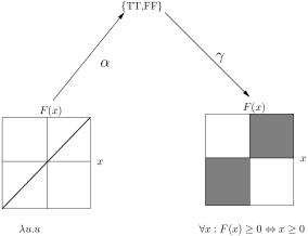
Figure 3: Abstraction and Concretization for the initial state for the example.

Proposition 4.1

For any pair of concrete state sets $S_{C}$ and $T_{C}$:

1. If $S_{C}\subseteq T_{C}$, then $\alpha(S_{C})\subseteq\alpha(T_{C})$.

2. $\alpha(S_{C})\cup\alpha(T_{C})=\alpha(S_{C}\cup T_{C})$.

These properties follow directly from the way we extended $\alpha$ from a single concrete state to a set of concrete states.

We define the concretization function $\gamma$ to require universal quantification over the index symbols. That is, for a set of abstract states $S_{A}\subseteq\Sigma_{{\cal P}}$, we let $\gamma(S_{A})$ be the following set of concrete states:

$$\gamma(S_{A})\;\;\;\doteq\;\;\;\left\{s|\forall\sigma_{\mbox{}\!{\cal X}}\in\Sigma_{{\cal X}}:\left\langle\boldsymbol{\phi}\right\rangle_{s\cdot\sigma_{\mbox{}\!{\cal X}}}\in S_{A}\right\}$$ (5)

Consider the Figure 2, where a set of abstract states $S_{A}$ has been concretized to a set of concrete states $\gamma(S_{A})$. It shows a concrete state $t$ that is not included in $\gamma(S_{A})$ because one of the states it abstracts to lies outside $S_{A}$. On the other hand, the concrete state $u$ is contained in $\gamma(S_{A})$ because $\alpha(u)\subseteq S_{A}$. One can provide an alternate definition of $\gamma$ as follows:

$$\gamma(S_{A})\;\;\;\doteq\;\;\;\left\{s|\alpha(s)\subseteq S_{A}\right\}$$ (6)

The universal quantifier in the definition of $\gamma$ has the consequence that the concretization function does not distribute over set union. In particular, we cannot view the concretization function as operating on individual abstract states, but rather as generating each concrete state from multiple abstract states.

Proposition 4.2

For any pair of abstract state sets $S_{A}$ and $T_{A}$:

1. If $S_{A}\subseteq T_{A}$, then $\gamma(S_{A})\subseteq\gamma(T_{A})$.

2. $\gamma(S_{A})\cup\gamma(T_{A})\subseteq\gamma(S_{A}\cup T_{A})$.

The first property follows from (5), while the second follows from the first.

Consider our example system with predicates $\phi_{\mathtt{p}}$ and $\phi_{\mathtt{q}}$. Table 1 shows some example abstract state sets $S_{A}$ and their concretizations $\gamma(S_{A})$. As the first three examples show, some (altogether 6) nonempty abstract state sets have empty concretizations, because they constrain $\mathtt{x}$ to be either always negative or always nonnegative. On the other hand, there are 9 abstract state sets having nonempty concretizations. We can see by this that the concretization function is based on the entire abstract state set and not just on the individual values. For example, the sets $\{\mbox{TF}\}$ and $\{\mbox{TT}\}$ have empty concretizations, but $\{\mbox{TF},\mbox{TT}\}$ concretizes to the set of all nonnegative functions.

Theorem 4.3

The functions $(\alpha,\gamma)$ form a Galois connection, i.e., for any sets of concrete states $S_{C}$ and abstract states $S_{A}$:

$$\alpha(S_{C})\subseteq S_{A}\;\Leftrightarrow\;S_{C}\subseteq\gamma(S_{A})$$ (7)

Proof.

(This is one of several logically equivalent formulations of a Galois connection [Cousot and Cousot (1977)].) The proof follows by observing that both the left and the right-hand sides of (7) hold precisely when for every $\sigma_{\mbox{}\!{\cal X}}\in\Sigma_{{\cal X}}$ and every $s\in S_{C}$, we have $\left\langle\boldsymbol{\phi}\right\rangle_{s\cdot\sigma_{\mbox{}\!{\cal X}}}\in S_{A}$. Let us prove the two directions:

1. If : Let $\alpha(S_{C})\subseteq S_{A}$. By the definition of $\alpha$ in (1), this implies that for every $s\in S_{C}$ and for interpretation $\sigma_{\mbox{}\!{\cal X}}\in\Sigma_{{\cal X}}$, $\left\langle\boldsymbol{\phi}\right\rangle_{s\cdot\sigma_{\mbox{}\!{\cal X}}}\in S_{A}$. By the definition of $\gamma$ in (5), $\gamma(S_{A})$ contains precisely those concrete states $s^{\prime}$ for which $\left\langle\boldsymbol{\phi}\right\rangle_{s^{\prime}\cdot\sigma_{\mbox{}\!{\cal X}}}\in S_{A}$, for every interpretation $\sigma_{\mbox{}\!{\cal X}}\in\Sigma_{{\cal X}}$. Thus, for every $s\in S_{C}$, $s\in\gamma(S_{A})$ and consequently, $S_{C}\subseteq\gamma(S_{A})$.

2. Only if : Let $S_{C}\subseteq\gamma(S_{A})$. Hence, by (5), for every $s\in S_{C}$, $\left\langle\boldsymbol{\phi}\right\rangle_{s\cdot\sigma_{\mbox{}\!{\cal X}}}\in S_{A}$, for every interpretation $\sigma_{\mbox{}\!{\cal X}}\in\Sigma_{{\cal X}}$. By the definition of $\alpha$ in (1), $\alpha(s)\in S_{A}$. Further, by extending $\alpha$ for the entire set $S_{C}$ by (3), we get $\alpha(S_{C})\subseteq S_{A}$.

∎

Alternately, the functions ($\alpha,\gamma$) form a Galois connection if they satisfy the following properties for any sets of concrete states $S_{C}$ and abstract states $S_{A}$:

$$S_{C}\;\; \subseteq \;\;\gamma(\alpha(S_{C})).$$ (8)

$$\alpha(\gamma(S_{A}))\;\; \subseteq \;\;S_{A}.$$ (9)

These properties can be derived from (7). Similarly, (7) can be derived from (8) and (9). The containment relation in both (8) and (9) can be proper. For example, the concrete state set consisting of the single function $\lambda\,u\mathbin{.}u$ abstracts to the state set $\mathtt{p}\Leftrightarrow\mathtt{q}$, which in turn concretizes to the set of all functions $f$ such that $f(u)\geq 0\Leftrightarrow u\geq 0$, for any argument $u$. This is clearly demonstrated in Fig 3. On the other hand, consider the set of abstract states represented by $\mathtt{p}\wedge\mathtt{q}$. This set of abstract states has an empty concretization (see Table 1), and thereby satisfies $\alpha(\gamma(S_{A}))\subset S_{A}$.

5 Abstract System

Predicate abstraction involves performing a reachability analysis over the abstract state space, where on each step we concretize the abstract state set via $\gamma$, apply the concrete next-state function, and then abstract the results via $\alpha$. We can view this process as performing reachability analysis on an abstract system having initial state set $Q^{0}_{A}\doteq\alpha(Q^{0}_{C})$ and a next-state function operating on sets: $N_{A}(S_{A})\doteq\alpha(N_{C}(\gamma(S_{A})))$. Note that there is no transition relation associated with this next-state function, since $\gamma$ cannot be viewed as operating on individual abstract states.

It can be seen that $N_{A}$ provides an abstract interpretation [Cousot and Cousot (1977)] of the concrete system:

1. $N_{A}$ is null-preserving: $N_{A}(\emptyset)=\emptyset$

2. $N_{A}$ is monotonic: $S_{A}\subseteq T_{A}\;\Rightarrow\;N_{A}(S_{A})\subseteq N_{A}(T_{A})$.

3. $N_{A}$ simulates $N_{C}$ (with a simulation relation defined by $\alpha$): $\alpha(N_{C}(S_{C}))\subseteq N_{A}(\alpha(S_{C}))$.

Theorem 5.1

$N_{A}$ provides an abstract interpretation of the concrete transition system $N_{C}$.

Proof.

Let us prove the three properties mentioned above:

1. This follows from the definition of $N_{A}$ and the fact that $\gamma(\emptyset)=\emptyset$, $N_{C}(\emptyset)=\emptyset$ and $\alpha(\emptyset)=\emptyset$.

2. By the definition of $N_{A}$, and using the fact that $\gamma$, $\alpha$ and $N_{C}$ are monotonic. $N_{C}$ is monotonic since it distributes over the elements of a set of concrete states, i.e. $N_{C}(S_{C})=\bigcup_{s\in S_{C}}N_{C}(s)$.

3. From (8), we know that $S_{C}\subseteq\gamma(\alpha(S_{C}))$. By the monotonicity of $N_{C}$, $N_{C}(S_{C})\subseteq N_{C}(\gamma(\alpha(S_{C})))$. Since $\alpha$ is monotonic, we have $\alpha(N_{C}(S_{C}))\subseteq\alpha(N_{C}(\gamma(\alpha(S_{C}))))$. Now applying the definition of $N_{A}$, we get the desired result.

∎

6 Reachability Analysis

Predicate abstraction involves performing a reachability analysis over the abstract state space, where on each step we concretize the abstract states via $\gamma$, apply the concrete transition relation, and then abstract the results via $\alpha$. In particular, define $R_{A}^{i}$, the set of states reached on step $i$ as:

$$R_{A}^{0} = Q^{0}_{A}$$ (10)

$$\displaystyle R_{A}^{i+1} = R_{A}^{i}\cup N_{A}(R_{A}^{i})$$ (11)

$$= \displaystyle R_{A}^{i}\;\cup\bigcup_{s\in\gamma(R_{A}^{i})}\;\;\bigcup_{t\in N_{C}(s)}\alpha(t)$$ (12)

Proposition 6.1

If $s$ is a reachable state in the concrete system such that ${\it depth}(s)\leq n$, then $\alpha(s)\subseteq R_{A}^{n}$.

Proof.

We prove this by induction on $n$. For $n=0$, the only concrete states having depth $0$ are those in $Q_{0}$, and by (10), these states are all included in $R_{A}^{0}$.

For a state $t$ having depth $k<n$, our induction hypothesis shows that $\alpha(t)\subseteq R_{A}^{n-1}$. Since $R_{A}^{n-1}\subseteq R_{A}^{n}$, we therefore have $\alpha(t)\subseteq R_{A}^{n}$.

Otherwise, suppose state $t$ has depth $n$. Then there must be some state $s$ having depth $n-1$ such that $t\in N_{C}(s)$. By the induction hypothesis, we must have $\alpha(s)\subseteq R_{A}^{n-1}$. By (8), we have $s\in\gamma(\alpha(s))$, and Proposition 4.2 then implies that $s\in\gamma(R_{A}^{n-1})$. By (12), we can therefore see that $\alpha(t)\subseteq R_{A}^{n}$. ∎

Since the abstract system is finite, there must be some $n$ such that $R_{A}^{n}=R_{A}^{n+1}$. The set of all reachable abstract states $R_{A}$ is then $R_{A}^{n}$.

Proposition 6.2

The abstract system computes an overapproximation of the set of reachable concrete states, i.e.,

$$\alpha(R_{C}) \subseteq R_{A}$$ (13)

Thus, even though determining the set of reachable concrete states would require examining paths of unbounded length, we can compute a conservative approximation to this set by performing a bounded reachability analysis on the abstract system.

Remark 6.3.

It is worth noting that we cannot use the standard “frontier set” optimization in our reachability analysis. This optimization, commonly used in symbolic model checking, considers only the newly reached states in computing the next set of reachable states. In our context, this would mean using the computation $R_{A}^{i+1}=R_{A}^{i}\cup N_{A}(R_{A}^{i}-R_{A}^{i-1})$ rather than that of (12). This optimization is not valid, due to the fact that $\gamma$, and therefore $N_{A}$, does not distribute over set union.

As an illustration, let us perform reachability analysis on our example system:

1. In the initial state, state element $\mathtt{F}$ is the identity function, which we have seen abstracts to the set represented by the formula $\mathtt{p}\Leftrightarrow\mathtt{q}$. This abstract state set concretizes to the set of functions $f$ satisfying $f(u)\geq 0\Leftrightarrow u\geq 0$. This is illustrated in Fig 3.

2. Let $h$ denote the value of $\mathtt{F}$ in the next state. If input $\mathtt{i}$ is $-1$, we would $h(-1)=f(0)\geq 0$, but we can still guarantee that $h(u)\geq 0$ for $u\geq 0$. This is illustrated in Fig 4. Applying the abstraction function, we get $R_{A}^{1}$ characterized by the formula $\mathtt{p}\lor\neg\mathtt{q}$ (see Table 1.)

3. For the second iteration, the abstract state set characterized by the formula $\mathtt{p}\lor\neg\mathtt{q}$ concretizes to the set of functions $f$ satisfying $f(u)\geq 0$ when $u\geq 0$, and this condition must hold in the next state as well. Applying the abstraction function to this set, we then get $R_{A}^{2}=R_{A}^{1}$, and hence the process has converged.

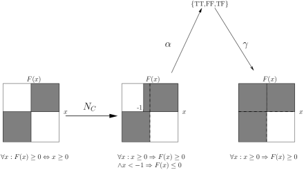
Figure 4: Reachability after 1 iteration for the example.

7 Verifying Safety Properties

A Boolean formula $\psi\in E({\cal P})$ can be viewed as defining a property of the abstract state space. Such a property is said to hold for the abstract system when it holds for every reachable abstract state. That is, $\left\langle\psi\right\rangle_{\sigma_{\mbox{}\!{\cal P}}}={\bf true}$ for all $\sigma_{\mbox{}\!{\cal P}}\in R_{A}$.

For Boolean formula $\psi\in E({\cal P})$, define the formula $\psi^{*}\in E({\cal V}\cup{\cal X})$ to be the result of substituting the predicate expression $\phi_{\mathtt{p}}$ for each predicate symbol $\mathtt{p}\in{\cal P}$. That is, viewing $\phi$ as a substitution, we have $\psi^{*}\doteq\psi\left[\phi/{\cal P}\right]$.

Proposition 7.1

For any formula $\psi\in E({\cal P})$, any concrete state $s$, and interpretation $\sigma_{\mbox{}\!{\cal X}}\in\Sigma_{{\cal X}}$, if $\sigma_{\mbox{}\!{\cal P}}=\left\langle\boldsymbol{\phi}\right\rangle_{s\cdot\sigma_{\mbox{}\!{\cal X}}}$, then $\left\langle\psi^{*}\right\rangle_{s\cdot\sigma_{\mbox{}\!{\cal X}}}=\left\langle\psi\right\rangle_{\sigma_{\mbox{}\!{\cal P}}}$.

This is a particular instance of Proposition 2.1.

We can view the formula $\psi^{*}$ as defining a property $\forall{\cal X}\psi^{*}$ of the concrete state space. This property is said to hold for concrete state $s$, written $\forall{\cal X}\psi^{*}(s)$, when $\left\langle\psi^{*}\right\rangle_{s\cdot\sigma_{\mbox{}\!{\cal X}}}={\bf true}$ for every $\sigma_{\mbox{}\!{\cal X}}\in\Sigma_{{\cal X}}$. The property is said to hold for the concrete system when $\forall{\cal X}\psi^{*}(s)$ holds for every reachable concrete state $s\in R_{C}$.

With our example system, letting formula $\psi\doteq\mathtt{p}\lor\neg\mathtt{q}$, and noting that $\mathtt{p}\lor\neg\mathtt{q}\;\equiv\;\mathtt{q}\Rightarrow\mathtt{p}$, we get as a property of state variable $\mathtt{F}$ that $\forall\mathtt{x}:\mathtt{x}\geq 0\Rightarrow\mathtt{F}(\mathtt{x})\geq 0$.

Proposition 7.2

Property $\forall{\cal X}\psi^{*}(s)$ holds for concrete state $s$ if and only if $\left\langle\psi\right\rangle_{\sigma_{\mbox{}\!{\cal P}}}={\bf true}$ for every $\sigma_{\mbox{}\!{\cal P}}\in\alpha(s)$.

This property follows from the definition of $\alpha$ (Equation 1) and Proposition 7.1.

Alternately, a Boolean $\psi\in E({\cal P})$ formula can also be viewed as characterizing a set of abstract states $\left\langle\psi\right\rangle\doteq\{\sigma_{\mbox{}\!{\cal P}}\;|\;\left\langle\psi\right\rangle_{\sigma_{\mbox{}\!{\cal P}}}={\bf true}\}$. Similarly, we can interpret the formula $\forall{\cal X}\psi^{*}$ as characterizing the set of concrete states $\left\langle\forall{\cal X}\psi^{*}\right\rangle\doteq\{s\;|\;\left\langle\forall{\cal X}\psi^{*}\right\rangle_{s}={\bf true}\}$.

Proposition 7.3

If $S_{C}\doteq\left\langle\forall{\cal X}\psi^{*}\right\rangle$ and $S_{A}\doteq\left\langle\psi\right\rangle$, then $S_{C}=\gamma(S_{A})$.

Proof.

Expanding the definition of $S_{C}$, we get

$$S_{C} = \{s\;|\;\forall\sigma_{\mbox{}\!{\cal X}}\in\Sigma_{{\cal X}}\;:\;\left\langle\psi^{*}\right\rangle_{s\cdot\sigma_{\mbox{}\!{\cal X}}}={\bf true}\}$$ (14)

$$= \{s\;|\;\forall\sigma_{\mbox{}\!{\cal X}}\in\Sigma_{{\cal X}}\;:\;\sigma_{\mbox{}\!{\cal P}}=\left\langle\boldsymbol{\phi}\right\rangle_{s\cdot\sigma_{\mbox{}\!{\cal X}}}\;\Rightarrow\;\left\langle\psi\right\rangle_{\sigma_{\mbox{}\!{\cal P}}}={\bf true}\}$$ (15)

$$= \{s\;|\;\forall\sigma_{\mbox{}\!{\cal X}}\in\Sigma_{{\cal X}}\;:\;\left\langle\boldsymbol{\phi}\right\rangle_{s\cdot\sigma_{\mbox{}\!{\cal X}}}\;\in S_{A}\}$$ (16)

Observe that (15) follows from (14) by expanding the definition of $S_{C}$ and (16) follows from (15) by using Proposition 7.1. ∎

The purpose of predicate abstraction is to provide a way to verify that a property $\forall{\cal X}\psi^{*}(s)$ holds for the concrete system based on the set of reachable abstract states.

Theorem 7.4

For a formula $\psi\in E({\cal P})$, if property $\psi$ holds for the abstract system, then property $\forall{\cal X}\psi^{*}$ holds for the concrete system.

Proof.

Consider an arbitrary concrete state $s\in R_{C}$ and an arbitrary interpretation $\sigma_{\mbox{}\!{\cal X}}\in\Sigma_{{\cal X}}$. If we let $\sigma_{\mbox{}\!{\cal P}}=\left\langle\boldsymbol{\phi}\right\rangle_{s\cdot\sigma_{\mbox{}\!{\cal X}}}$, then by the definition of $\alpha$ (Equation 1), we must have $\sigma_{\mbox{}\!{\cal P}}\in\alpha(s)$. By Propositions 4.1 and 6.2, we therefore have

$$\sigma_{\mbox{}\!{\cal P}}\;\;\;\in\;\;\;\alpha(s)\;\;\;\subseteq\;\;\;\alpha(R_{C})\;\;\;\subseteq\;\;\;R_{A}$$

By the premise of the theorem we have $\left\langle\psi\right\rangle_{\sigma_{\mbox{}\!{\cal P}}}={\bf true}$, and by Proposition 7.1, we have $\left\langle\psi^{*}\right\rangle_{s\cdot\sigma_{\mbox{}\!{\cal X}}}=\left\langle\psi\right\rangle_{\sigma_{\mbox{}\!{\cal P}}}={\bf true}$. This is precisely the condition required for the property $\forall{\cal X}\psi^{*}$ to hold for the concrete system. ∎

Thus, the abstract reachability analysis on our example system does indeed prove the property that any value $f$ of state variable $\mathtt{F}$ satisfies $\forall x:x\geq 0\Rightarrow f(x)\geq 0$.

Using predicate abstraction, we can possibly get a false negative result, where we fail to verify a property $\forall{\cal X}\psi^{*}$, even though it holds for the concrete system, because the given set of predicates does not adequately capture the characteristics of the system that ensure the desired property. Thus, this method of verifying properties is sound, but possibly incomplete.

For example, any reachable state $f$ of our example system satisfies $\forall x:f(x)<0\Rightarrow f(-x)\geq-x$, but our reachability analysis cannot show this.

We can, however, precisely characterize the class of properties for which this form of predicate analysis is both sound and complete. A property $\forall{\cal X}\psi^{*}$ is said to be inductive for the concrete system when it satisfies the following two properties:

1. Every initial state $s\in Q_{0}$ satisfies $\forall{\cal X}\psi^{*}(s)$.

2. For every pair of concrete states $(s,t)$, such that $t\in N_{C}(s)$, if $\forall{\cal X}\psi^{*}(s)$ holds, then so does $\forall{\cal X}\psi^{*}(t)$.

Proposition 7.5

If $\forall{\cal X}\psi^{*}$ is inductive, then $\forall{\cal X}\psi^{*}$ holds for the concrete system.

This proposition follows by induction on the state sequence leading to each reachable state.

Let $\rho_{A}$ be a formula that exactly characterizes the set of reachable abstract states. That is, $\left\langle\rho_{A}\right\rangle=R_{A}$.

Lemma 7.6

$\forall{\cal X}\rho_{A}^{*}$ is inductive.

Proof.

By definition, $\left\langle\rho_{A}\right\rangle_{\sigma_{\mbox{}\!{\cal P}}}={\bf true}$ if and only if $\sigma_{\mbox{}\!{\cal P}}\in R_{A}$, and so by Proposition 7.2, $\forall{\cal X}\rho_{A}^{*}(s)$ holds for concrete state $s$ if and only if $\alpha(s)\subseteq R_{A}$.

We can see that the first requirement is satisfied for any $s\in Q_{0}$, since $\alpha(s)\subseteq\alpha(Q_{0})\subseteq R_{A}$ and therefore $\forall{\cal X}\rho_{A}^{*}(s)$ holds by Proposition 7.2.

Now suppose there is a state $t\in N_{C}(s)$ and $\forall{\cal X}\rho_{A}^{*}(s)$ holds. Then we must have $\alpha(s)\subseteq R_{A}^{i}$ for some $i\geq 0$. From (8), we have $s\in\gamma(\alpha(s))\subseteq\gamma(R_{A}^{i})$, and therefore, by (12), $\alpha(t)\subseteq R_{A}^{i+1}\subseteq R_{A}$. Thus, the second requirement is satisfied. ∎

Lemma 7.7

If $\forall{\cal X}\psi^{*}$ is inductive, then $\psi$ holds for the abstract system.

Proof.

We will prove by induction on $i$ that $\left\langle\psi\right\rangle_{\sigma_{\mbox{}\!{\cal P}}}={\bf true}$ for every $\sigma_{\mbox{}\!{\cal P}}\in R_{A}^{i}$. From the definition of $R_{A}$, it then follows that $\left\langle\psi\right\rangle_{\sigma_{\mbox{}\!{\cal P}}}={\bf true}$ for every $\sigma_{\mbox{}\!{\cal P}}\in R_{A}$, and therefore $\psi$ holds for the abstract system.

For the case of $i=0$, (10) indicates that $R_{A}^{0}=\alpha(Q_{0})$. Thus, by the definition of $\alpha$ (Equation 1) for every $\sigma_{\mbox{}\!{\cal P}}\in R_{A}^{0}$, there must be a state $s$ and an interpretation $\sigma_{\mbox{}\!{\cal X}}\in\Sigma_{{\cal X}}$ such that $\sigma_{\mbox{}\!{\cal P}}=\left\langle\boldsymbol{\phi}\right\rangle_{s\cdot\sigma_{\mbox{}\!{\cal X}}}$. By the first property of an inductive predicate and by Proposition 7.1, we have $\left\langle\psi\right\rangle_{\sigma_{\mbox{}\!{\cal P}}}=\left\langle\psi^{*}\right\rangle_{s\cdot\sigma_{\mbox{}\!{\cal X}}}={\bf true}$.

Now suppose that $\left\langle\psi\right\rangle_{\sigma_{\mbox{}\!{\cal P}}}={\bf true}$ for all $\sigma_{\mbox{}\!{\cal P}}\in R_{A}^{i}$. Consider an element $\tau_{\mbox{}\!{\cal P}}\in R_{A}^{i+1}$. If $\tau_{\mbox{}\!{\cal P}}\in R_{A}^{i}$, then our induction hypothesis shows that $\left\langle\psi\right\rangle_{\tau_{\mbox{}\!{\cal P}}}={\bf true}$. Otherwise, by (12), and the definitions of $\alpha$ (Equation 1), the transition relation $N_{C}$, and $\gamma$ (Equation 5), there must be concrete states $s$ and $t$ satisfying:

1. $\tau_{\mbox{}\!{\cal P}}\in\alpha(t)$. That is, $\tau_{\mbox{}\!{\cal P}}=\left\langle\boldsymbol{\phi}\right\rangle_{t\cdot\tau_{\mbox{}\!{\cal X}}}$ for some $\tau_{\mbox{}\!{\cal X}}\in\Sigma_{{\cal X}}$.

2. $t\in N_{C}(s)$.

3. $s\in\gamma(R_{A}^{i})$. That is, for all $\sigma_{\mbox{}\!{\cal X}}\in\Sigma_{{\cal X}}$, if $\sigma_{\mbox{}\!{\cal P}}\doteq\left\langle\boldsymbol{\phi}\right\rangle_{s\cdot\sigma_{\mbox{}\!{\cal X}}}$, then $\sigma_{\mbox{}\!{\cal P}}\in R_{A}^{i}$.

By Proposition 7.1 we have $\left\langle\psi^{*}\right\rangle_{s\cdot\sigma_{\mbox{}\!{\cal X}}}=\left\langle\psi\right\rangle_{\sigma_{\mbox{}\!{\cal P}}}={\bf true}$, and therefore $\forall{\cal X}\psi^{*}(s)$ holds. By the second property of an inductive predicate, $\forall{\cal X}\psi^{*}(t)$ must also hold. Applying Proposition 7.1 once again, we therefore have $\left\langle\psi\right\rangle_{\tau_{\mbox{}\!{\cal P}}}=\left\langle\psi^{*}\right\rangle_{t\cdot\tau_{\mbox{}\!{\cal X}}}={\bf true}$. This completes our induction. ∎

This lemma simply shows that if we present our predicate abstraction engine with a fully formed induction hypothesis, then it will be able to perform the induction proof. But, it has important consequences.

For a formula $\psi\in E({\cal P})$ and a predicate set $\phi$, the property $\forall{\cal X}\psi^{*}$ is said to have an induction proof over $\phi$ when there is some formula $\chi\in E({\cal P})$, such that $\chi\Rightarrow\psi$ and $\forall{\cal X}\chi^{*}$ is inductive. That is, there is some way to strengthen $\psi$ into a formula $\chi$ that can be used to prove the property by induction.

Theorem 7.8

A formula $\psi\in E({\cal P})$ is a property of the abstract system if and only if the concrete property $\forall{\cal X}\psi^{*}$ has an induction proof over the predicate set $\phi$.

Proof.

Suppose there is a formula $\chi$ such that $\forall{\cal X}\chi^{*}$ is inductive. Then by Lemma 7.7, we know that $\chi$ holds in the abstract system, and when $\chi\Rightarrow\psi$, we can infer that $\psi$ holds in the abstract system.

On the other hand, suppose that $\psi$ holds in the abstract system. Then the formula $\rho_{A}$ (characterizing the set of all reachable abstract states) satisfies $\rho_{A}\Rightarrow\psi$ and $\forall{\cal X}\rho_{A}^{*}$ is inductive. Hence $\forall{\cal X}\psi^{*}$ has an induction proof over $\phi$. ∎

This theorem precisely characterizes the capability of our formulation of predicate abstraction — it can prove any property that can be strengthened into an induction hypothesis using some combination of the predicates. Thus, if we fail to verify a system using this form of predicate abstraction, we can conclude that either 1) the system does not satisfy the property, or 2) we did not provide an adequate set of predicates out of which the predicate abstraction engine could construct a universally quantified induction hypothesis.

Corollary 7.9

The property $\forall{\cal X}\rho_{A}^{*}$ is the strongest inductive invariant for the concrete system of the form $\forall{\cal X}\chi^{*}$, where $\chi\in E({\cal P})$. Alternately, for any other inductive property $\forall{\cal X}\chi^{*}$, where $\chi\in E({\cal P})$, $\forall{\cal X}\rho_{A}^{*}\Rightarrow\forall{\cal X}\chi^{*}$.

Proof.

The proof follows easily from Theorem 7.8, the fact that $\rho_{A}\Rightarrow\chi$ whenever $\chi$ is a property of the abstract state space, Proposition 7.3 and Proposition 4.2. ∎

Remark 7.10.

To fully automate the process of generating invariants, we need to further discover the predicates automatically. Other predicate abstraction tools [Ball et al. (2001), Henzinger et al. (2002), Chaki et al. (2003), Das and Dill (2002)] generate new predicates based on ruling out spurious counterexample traces from the abstract model. This approach cannot be used directly in our context, since our abstract system cannot be viewed as a state transition system, and so there is no way to characterize a counterexample by a single state sequence. In this paper, we do not address the issue of discovering the indexed predicates: we provide a syntactic heuristic based on the weakest precondition transformer in a separate work [Lahiri and Bryant (2004)].

8 Quantifier Instantiation

For many subsets of first-order logic, there is no complete method for handling the universal quantifier introduced in function $\gamma$ (Equation 5). For example, in a logic with uninterpreted functions and equality, determining whether a universally quantified formula is satisfiable is undecidable [Börger et al. (1997)]. Instead, we concretize abstract states by considering some limited subset of the interpretations of the index symbols, each of which is defined by a substitution for the symbols in ${\cal X}$. Our tool automatically generates candidate substitutions based on the subexpressions that appear in the predicate and next-state expressions. Details of the quantifier instantiation heuristic can be found in an earlier work [Lahiri et al. (2002)]. These subexpressions can contain symbols in ${\cal V}$, ${\cal X}$, and ${\cal I}$. These instantiated versions of the formulas enable the verifier to detect specific cases where the predicates can be applied.

More precisely, let $\pi$ be a substitution assigning an expression $\pi_{\mathtt{x}}\in E({\cal V}\cup{\cal X}\cup{\cal I})$ for each $\mathtt{x}\in{\cal X}$. Then $\phi_{\mathtt{p}}\left[\pi/{\cal X}\right]$ will be a Boolean expression over symbols ${\cal V}$, ${\cal X}$, and ${\cal I}$ that represents some instantiation of predicate $\phi_{\mathtt{p}}$.

For a set of substitutions $\Pi$ and interpretations $\sigma_{\mbox{}\!{\cal X}}\in\Sigma_{{\cal X}}$ and $\sigma_{\mbox{}\!{\cal I}}\in\Sigma_{{\cal I}}$, we define the concretization function $\gamma_{\Pi}$ as:

$$\gamma_{\Pi}(S_{A},\sigma_{\mbox{}\!{\cal X}},\sigma_{\mbox{}\!{\cal I}})\;\;\;\doteq\;\;\;\left\{s|\forall\pi\in\Pi:\left\langle\boldsymbol{\phi}\left[\boldsymbol{\pi}/{\cal X}\right]\right\rangle_{s\cdot\sigma_{\mbox{}\!{\cal X}}\cdot\sigma_{\mbox{}\!{\cal I}}}\in S_{A}\right\}$$ (17)

Proposition 8.1

For any abstract state set $S_{A}$ and interpretations $\sigma_{\mbox{}\!{\cal X}}\in\Sigma_{{\cal X}}$ and $\sigma_{\mbox{}\!{\cal I}}\in\Sigma_{{\cal I}}$:

1. $\gamma(S_{A})\subseteq\gamma_{\Pi}(S_{A},\sigma_{\mbox{}\!{\cal X}},\sigma_{\mbox{}\!{\cal I}})$ for any set of substitutions $\Pi$.

2. $\gamma_{\Pi}(S_{A},\sigma_{\mbox{}\!{\cal X}},\sigma_{\mbox{}\!{\cal I}})\subseteq\gamma_{\Pi^{\prime}}(S_{A},\sigma_{\mbox{}\!{\cal X}},\sigma_{\mbox{}\!{\cal I}})$ for any pair of substitution sets $\Pi$ and $\Pi^{\prime}$ satisfying $\Pi\supseteq\Pi^{\prime}$.

3. For any abstract state set $T_{A}$, if $S_{A}\subseteq T_{A}$, then $\gamma_{\Pi}(S_{A},\sigma_{\mbox{}\!{\cal X}},\sigma_{\mbox{}\!{\cal I}})\subseteq\gamma_{\Pi}(T_{A},\sigma_{\mbox{}\!{\cal X}},\sigma_{\mbox{}\!{\cal I}})$, for any set of substitutions $\Pi$.

These properties follow directly from the definitions of $\gamma$ and $\gamma_{\Pi}$ and Proposition 2.1.

Proposition 8.2

For any concrete state set $S_{C}$, set of substitutions $\Pi$, and interpretations $\sigma_{\mbox{}\!{\cal X}}\in\Sigma_{{\cal X}}$ and $\sigma_{\mbox{}\!{\cal I}}\in\Sigma_{{\cal I}}$:

$$S_{C}\quad\subseteq\quad\gamma_{\Pi}(\alpha(S_{C}),\sigma_{\mbox{}\!{\cal X}},\sigma_{\mbox{}\!{\cal I}}).$$ (18)

This property follows directly from Theorem 4.3 and Proposition 8.1. It shows that for a given interpretation $\sigma_{\mbox{}\!{\cal X}}$ and $\sigma_{\mbox{}\!{\cal I}}$, the functions $(\alpha,\gamma_{\Pi})$ satisfy one of the properties of a Galois connection (Equation 8), but they need not satisfy the other (Equation 9). For example, when $\Pi=\emptyset$, the quantified condition of (17) becomes vacuous, and hence $\gamma_{\Pi}(S_{A},\sigma_{\mbox{}\!{\cal X}},\sigma_{\mbox{}\!{\cal I}})=\Sigma_{{\cal V}}$.

We can use $\gamma_{\Pi}$ as an approximation to $\gamma$ in defining the behavior of the abstract system. That is, define $N_{\Pi}$ over sets of abstract states as:

$$N_{\Pi}(S_{A}) = \left\{\left\langle\phi\left[\delta/{\cal V}\right]\right\rangle_{s\cdot\sigma_{\mbox{}\!{\cal X}}\cdot\sigma_{\mbox{}\!{\cal I}}}|\sigma_{\mbox{}\!{\cal X}}\in\Sigma_{{\cal X}},\sigma_{\mbox{}\!{\cal I}}\in\Sigma_{{\cal I}},s\in\gamma_{\Pi}(S_{A},\sigma_{\mbox{}\!{\cal X}},\sigma_{\mbox{}\!{\cal I}})\right\}$$ (19)

$$= \bigcup_{\sigma_{\mbox{}\!{\cal X}}\in\Sigma_{{\cal X}}}\bigcup_{\sigma_{\mbox{}\!{\cal I}}\in\Sigma_{{\cal I}}}\bigcup_{s\in\gamma_{\pi}(S_{A},\sigma_{\mbox{}\!{\cal X}},\sigma_{\mbox{}\!{\cal I}})}\left\{\left\langle\phi\left[\delta/{\cal V}\right]\right\rangle_{s\cdot\sigma_{\mbox{}\!{\cal X}}\cdot\sigma_{\mbox{}\!{\cal I}}}\right\}$$ (20)

Observe in this equation that $\phi_{\mathtt{p}}\left[\delta/{\cal V}\right]$ is an expression describing the evaluation of predicate $\phi_{\mathtt{p}}$ in the next state.

It can be seen that $N_{\Pi}(S_{A})\supseteq N_{A}(S_{A})$ for any set of abstract states $S_{A}$. As long as $\Pi$ is nonempty (required to guarantee that $N_{\Pi}$ is null-preserving), it can be shown that the system defined by $N_{\Pi}$ is an abstract interpretation of the concrete system:

1. $N_{\Pi}(\emptyset)=\emptyset$, if $\Pi$ is nonempty.

2. $N_{\Pi}$ is monotonic: This follows from the definition of $N_{\Pi}$ in (20) and Proposition 8.1.

3. $\alpha(N_{C}(S_{C}))\subseteq N_{\Pi}(\alpha(S_{C}))$: This follows from the fact that $\alpha(N_{C}(S_{C}))\subseteq N_{A}(\alpha(S_{C}))$ and $N_{A}(S_{A})\subseteq N_{\Pi}(S_{A})$.

We can therefore perform reachability analysis:

$$R_{\Pi}^{0} = Q^{0}_{A}$$ (21)

$$\displaystyle R_{\Pi}^{i+1} = \displaystyle R_{\Pi}^{i}\cup N_{\Pi}(R_{\Pi}^{i})$$ (22)

These iterations will converge to a set $R_{\Pi}$.

Proposition 8.3

1. $R_{A}\subseteq R_{\Pi}$ for any set of substitutions $\Pi$.

2. $R_{\Pi}\subseteq R_{\Pi^{\prime}}$ for any pair of substitution sets $\Pi$ and $\Pi^{\prime}$ satisfying $\Pi\supseteq\Pi^{\prime}$.

To see the first property, consider the following way of expressing the equation for $R_{A}^{i+1}$ (12) using the alternative equation for $\alpha$ (4), and rearranging the order of the union operations:

$$R_{A}^{i+1} = \displaystyle R_{A}^{i}\;\cup\bigcup_{\sigma_{\mbox{}\!{\cal X}}\in\Sigma_{{\cal X}}}\;\;\bigcup_{\sigma_{\mbox{}\!{\cal I}}\in\Sigma_{{\cal I}}}\;\;\bigcup_{s\in\gamma(R_{A}^{i})}\;\;\left\{\left\langle\phi\left[\delta/{\cal V}\right]\right\rangle_{s\cdot\sigma_{\mbox{}\!{\cal X}}\cdot\sigma_{\mbox{}\!{\cal I}}}\right\}$$

The property then follows by Proposition 8.1, using induction on $i$. The second property also follows by Proposition 8.1 using induction on $i$.

Theorem 8.4

For a formula $\psi\in E({\cal P})$, if $\left\langle\psi\right\rangle_{\sigma_{\mbox{}\!{\cal P}}}={\bf true}$ for every $\sigma_{\mbox{}\!{\cal P}}\in R_{\Pi}$, then property $\forall{\cal X}\psi^{*}$ holds for the concrete system.

Proof.

Since $\left\langle\psi\right\rangle_{\sigma_{\mbox{}\!{\cal P}}}={\bf true}$ for every $\sigma_{\mbox{}\!{\cal P}}\in R_{\Pi}$ and $R_{A}\subseteq R_{\Pi}$ (by Proposition 8.3), $\left\langle\psi\right\rangle_{\sigma_{\mbox{}\!{\cal P}}}={\bf true}$ for every $\sigma_{\mbox{}\!{\cal P}}\in R_{A}$. Hence by Theorem 7.4, the property $\forall{\cal X}\psi^{*}$ holds for the concrete system.

∎

This demonstrates that using quantifier instantiation during reachability analysis yields a sound verification technique. However, when the tool fails to verify a property, it could mean, in addition to the two possibilities listed earlier, that 3) it used an inadequate set of instantiations, or 4) that the property cannot be proved by any bounded quantifier instantiation.

9 Symbolic Formulation of Reachability Analysis

We are now ready to express the reachability computation symbolically, where each step involves finding the set of satisfying solutions to a quantified CLU formula. We will then see how this can be converted into a problem of finding satisfying solutions to a Boolean formula.

On each step, we generate a Boolean formula $\rho_{\Pi}^{i}$, that characterizes $R_{\Pi}^{i}$. That is $\left\langle\rho_{\Pi}^{i}\right\rangle=R_{\Pi}^{i}$. The formulas directly encode the approximate reachability computations of (21) and (22).

Observe that by composing the predicate expressions with the initial state expressions, $\phi\left[q^{0}/{\cal V}\right]$, we get a set of predicates over the initial state symbols ${\cal J}$ indicating the conditions under which the predicates hold in the initial state. We can therefore start the reachability analysis by finding solutions to the formula

$$\rho_{\Pi}^{0}({\cal P}) = \displaystyle{\exists{\cal X}\exists{\cal J}\bigwedge_{\mathtt{p}\in{\cal P}}\mathtt{p}\Leftrightarrow\phi\left[q^{0}/{\cal V}\right]}$$ (23)

Proposition 9.1

$\left\langle\rho_{\Pi}^{0}\right\rangle=Q^{0}_{A}$

Let us understand the expression $\rho_{\Pi}^{0}$ by showing why it represents $Q^{0}_{A}$. Expanding the definition of $Q^{0}_{A}$, we get:

$$Q^{0}_{A}=\bigcup_{\sigma_{\mbox{}\!{\cal X}}\in\Sigma_{{\cal X}}}\bigcup_{s\in Q^{0}_{C}}\left\{\left\langle\boldsymbol{\phi}\right\rangle_{s\cdot\sigma_{\mbox{}\!{\cal X}}}\right\}$$ (24)

Again, $Q^{0}_{C}=\bigcup_{\sigma_{\mbox{}\!{\cal J}}\in\Sigma_{{\cal J}}}\left\{\left\langle q^{0}\right\rangle_{\sigma_{\mbox{}\!{\cal J}}}\right\}$. Using Proposition 2.1, we can rewrite (24) as:

$$Q^{0}_{A}=\bigcup_{\sigma_{\mbox{}\!{\cal X}}\in\Sigma_{{\cal X}}}\bigcup_{\sigma_{\mbox{}\!{\cal J}}\in\Sigma_{{\cal J}}}\left\{\left\langle\phi\left[q^{0}/{\cal V}\right]\right\rangle_{\sigma_{\mbox{}\!{\cal J}}\cdot\sigma_{\mbox{}\!{\cal X}}}\right\}$$ (25)

To generate a formula for the next-state computation, we first generate a formula for $\gamma_{\pi}(R_{\Pi}^{i},\sigma_{\mbox{}\!{\cal X}},\sigma_{\mbox{}\!{\cal I}})$ by forming a conjunction over each substitution in $\Pi$, where we compose the current-state formula with the predicate expressions and with each substitution $\pi$: $\bigwedge_{\pi\in\Pi}\left(\rho_{\Pi}^{i}\left[\phi/{\cal P}\right]\right)\left[\pi/{\cal X}\right]$.

The formula for the next-state computation combines the alternate definition of $N_{\Pi}$ (20) and the formula for $\gamma_{\Pi}$ above:

$$\rho_{\Pi}^{i+1}({\cal P}) = \displaystyle{\rho_{\Pi}^{i}({\cal P})\;\lor\;}$$ (26)

$$\exists{\cal V}\exists{\cal X}\exists{\cal I}\displaystyle{\left(\bigwedge_{\pi\in\Pi}\left(\rho_{\Pi}^{i}\left[\phi/{\cal P}\right]\right)\left[\pi/{\cal X}\right]\;\;\land\;\;\bigwedge_{\mathtt{p}\in{\cal P}}\mathtt{p}\Leftrightarrow\phi_{\mathtt{p}}\left[\delta/{\cal V}\right]\right)}.$$

To understand the quantified term in this equation, note that the left-hand term is the formula for $\gamma_{\Pi}(\rho_{\Pi}^{i},\sigma_{\mbox{}\!{\cal X}},\sigma_{\mbox{}\!{\cal I}})$, while the right-hand term expresses the conditions under which each abstract state variable $\mathtt{p}$ will match the value of the corresponding predicate in the next state.

Proposition 9.2

$\left\langle\rho_{\Pi}^{i+1}\right\rangle=R_{\Pi}^{i+1}$

Let us see how this symbolic formulation would perform reachability analysis for our example system. Recall that our system has two predicates $\phi_{\mathtt{p}}\doteq\mathtt{F}(\mathtt{x})\geq 0$ and $\phi_{\mathtt{q}}\doteq\mathtt{x}\geq 0$. In the initial state, $\mathtt{F}$ is the function $\lambda\,u\mathbin{.}u$, and therefore $\phi_{\mathtt{p}}\left[q^{0}/{\cal V}\right]$ simply becomes $\mathtt{x}\geq 0$. Equation (23) then becomes $\exists\mathtt{x}\left[(\mathtt{p}\Leftrightarrow\mathtt{x}\geq 0)\land(\mathtt{q}\Leftrightarrow\mathtt{x}\geq 0)\right]$, which reduces to $\mathtt{p}\Leftrightarrow\mathtt{q}$.

Now let us perform the first iteration. For our instantiations we require two substitutions $\pi$ and $\pi^{\prime}$ with $\pi_{\mathtt{x}}=\mathtt{x}$ and $\pi^{\prime}_{\mathtt{x}}=\mathtt{i}\!+\!1$. For $\rho_{\Pi}^{0}(\mathtt{p},\mathtt{q})=\mathtt{p}\Leftrightarrow\mathtt{q}$, the left-hand term of (26) instantiates to $(\mathtt{F}(\mathtt{x})\geq 0\Leftrightarrow\mathtt{x}\geq 0)\land(\mathtt{F}(\mathtt{i}\!+\!1)\geq 0\Leftrightarrow\mathtt{i}\!+\!1\geq 0)$. Substituting $\lambda\,u\mathbin{.}\mbox{{\rm{\it ITE}}}(u=\mathtt{i},\,\mathtt{F}(\mathtt{i}\!+\!1),\,\mathtt{F}(u))$ for $\mathtt{F}$ in $\phi_{\mathtt{p}}$ gives $(\mathtt{x}\!=\!\mathtt{i}\land\mathtt{F}(\mathtt{i}\!+\!1)\geq 0)\lor(\mathtt{x}\!\not=\!\mathtt{i}\land\mathtt{F}(\mathtt{x})\geq 0)$.

The quantified portion of (26) for $\rho_{\Pi}^{1}(\mathtt{p},\mathtt{q})$ then becomes:

$$\exists\;\mathtt{F},\mathtt{x},\mathtt{i}:\left(\begin{array}[]{ll}&\mathtt{F}(\mathtt{x})\geq 0\Leftrightarrow\mathtt{x}\geq 0\;\;\land\;\;\mathtt{F}(\mathtt{i}\!+\!1)\geq 0\Leftrightarrow\mathtt{i}\!+\!1\geq 0\\ \land&\mathtt{p}\Leftrightarrow[(\mathtt{x}\!=\!\mathtt{i}\land\mathtt{F}(\mathtt{i}\!+\!1)\geq 0)\lor(\mathtt{x}\!\not=\!\mathtt{i}\land\mathtt{F}(\mathtt{x})\geq 0)]\\ \land&\mathtt{q}\Leftrightarrow\mathtt{x}\geq 0\end{array}\right)$$ (27)

The only values of $\mathtt{p}$ and $\mathtt{q}$ where this formula cannot be satisfied is when $\mathtt{p}$ is false and $\mathtt{q}$ is true.

As shown in [Lahiri et al. (2003)], we can generate the set of solutions to (23) and (26) by first transforming the formulas into equivalent Boolean formulas and then performing quantifier elimination to remove all Boolean variables other than those in ${\cal P}$. This quantifier elimination is similar to the relational product operation used in symbolic model checking and can be solved using either BDD or SAT-based methods.

10 Using a SAT Solver to Perform Reachability Analysis

Observe that (26) has a general form $\chi^{\prime}({\cal P})=\chi({\cal P})\lor\exists{\cal A}\,\theta({\cal A},{\cal P})$, where $\theta$ is a quantifier-free CLU formula, ${\cal A}$ contains Boolean, integer, function, and predicate symbols, and ${\cal P}$ contains only Boolean symbols. Several methods (including those in [Bryant et al. (2002b), Strichman et al. (2002), Bryant et al. (2002a)]) have been developed to transform a quantifier-free CLU formula $\theta({\cal A},{\cal P})$ into a Boolean formula $\tilde{\theta}(\tilde{{\cal A}},{\cal P})$, where $\tilde{{\cal A}}$ is now a set of Boolean variables, in a way that preserves satisfiability.

By taking care [Lahiri et al. (2003)], this transformation can be performed in a way that preserves the set of satisfying solutions for the symbols in ${\cal P}$. That is:

$$\{\sigma_{\mbox{}\!{\cal P}}|\exists\sigma_{\mbox{}\!{\cal A}}:\left\langle\theta\right\rangle_{\sigma_{\mbox{}\!{\cal A}}\cdot\sigma_{\mbox{}\!{\cal P}}}={\bf true}\}\;\;=\;\;\{\sigma_{\mbox{}\!{\cal P}}|\exists\sigma_{\mbox{}\!\tilde{{\cal A}}}:\left\langle\tilde{\theta}\right\rangle_{\sigma_{\mbox{}\!\tilde{{\cal A}}}\cdot\sigma_{\mbox{}\!{\cal P}}}={\bf true}\}$$ (28)

Based on such a transformation, we can generate a Boolean formula for $\chi^{\prime}$ by repeatedly calling a Boolean SAT solver, yielding one solution with each call. In this presentation, we consider an interpretation $\sigma_{\mbox{}\!{\cal P}}$ to represent a Boolean formula consisting of a conjunction of literals: $\mathtt{p}$ when $\sigma_{\mbox{}\!{\cal P}}(\mathtt{p})={\bf true}$ and $\neg\mathtt{p}$ when $\sigma_{\mbox{}\!{\cal P}}(\mathtt{p})={\bf false}$. Starting with $\chi^{\prime}=\chi$, and $\tilde{\theta}^{\prime}=\tilde{\theta}\land\neg\chi$, we perform iterations:

$$\sigma_{\mbox{}\!{\cal A}},\sigma_{\mbox{}\!{\cal P}} \leftarrow {\it SATSolve}(\tilde{\theta}^{\prime})$$

$$\chi^{\prime} \leftarrow \chi^{\prime}\lor\sigma_{\mbox{}\!{\cal P}}$$

$$\tilde{\theta}^{\prime} \leftarrow \tilde{\theta}^{\prime}\land\neg\sigma_{\mbox{}\!{\cal P}}$$

until $\tilde{\theta}^{\prime}$ is unsatisfiable.

To illustrate this process, let us solve (27) to perform the first iteration of reachability analysis on our example system. We can translate the right-hand term into Boolean form by introducing Boolean variables $\mathtt{a}$, $\mathtt{b}$, $\mathtt{c}$, $\mathtt{d}$ and $\mathtt{e}$ encoding the predicates $\mathtt{F}(\mathtt{x})\geq 0$, $\mathtt{x}\geq 0$, $\mathtt{F}(\mathtt{i}\!+\!1)\geq 0$, $\mathtt{\mathtt{i}\!+\!1}\geq 0$, and $\mathtt{x}=\mathtt{i}$, respectively.

The portion of (27) within square brackets then becomes

$$\mathtt{a}\Leftrightarrow\mathtt{b}\land\mathtt{c}\Leftrightarrow\mathtt{d}\land(\mathtt{p}\Leftrightarrow\left[(\mathtt{e}\land\mathtt{c})\lor(\neg\mathtt{e}\land\mathtt{a})\right])\land(\mathtt{q}\Leftrightarrow\mathtt{b}).$$

To this, let us add the consistency constraint: $\mathtt{e}\land\mathtt{b}\Rightarrow\mathtt{d}$ (encoding the property that $\mathtt{x}\!=\!\mathtt{i}\land\mathtt{x}\geq 0\Rightarrow\mathtt{i}\!+\!1\geq 0$). Although the translation schemes will add a lot more constraints (e.g., those involving uninterpreted function symbol), the above constraint is sufficient to preserve the property described in (28). For simplicity, we will not describe the other constraints that would be added by the algorithms in  [Lahiri et al. (2003)]. Finally, all the symbols apart from $\mathtt{p}$ and $\mathtt{q}$ are existentially quantified out.

It is easy to verify that the equation above with the consistency constraint is unsatisfiable only for the assignment when $\mathtt{p}$ is false and $\mathtt{q}$ is true.

11 Axioms

As a special class of predicates, we may have some that are to hold at all times. For example, we could have an axiom $\mathtt{f}(\mathtt{x})>0$ to indicate that function $\mathtt{f}$ is always positive, or $\mathtt{f}(\mathtt{y},\mathtt{z})=\mathtt{f}(\mathtt{z},\mathtt{y})$ to indicate that $\mathtt{f}$ is commutative. Typically, we want these predicates to be individually quantified, but we can ensure this by defining each of them over a unique set of index symbols, as we have done in the above examples.

We can add this feature to our analysis by identifying a subset ${\cal Q}$ of the predicate symbols ${\cal P}$ to be axioms. We then want to restrict the analysis to states where the axiomatic predicates hold. Let Let $\Sigma_{{\cal P}}^{{\cal Q}}$ denote the set of abstract states $\sigma_{\mbox{}\!{\cal P}}$ where $\sigma_{\mbox{}\!{\cal P}}(\mathtt{p})={\bf true}$ for every $\mathtt{p}\in{\cal Q}$. Then we can apply this restriction by redefining $\alpha(s)$ (Equation 1) for concrete state $s$ to be:

$$\alpha(s) \doteq \left\{\left\langle\boldsymbol{\phi}\right\rangle_{s\cdot\sigma_{\mbox{}\!{\cal X}}}|\sigma_{\mbox{}\!{\cal X}}\in\Sigma_{{\cal X}}\right\}\cap\Sigma_{{\cal P}}^{{\cal Q}}$$ (29)

and then using this definition in the extension of $\alpha$ to sets (Equation 3), the formulation of the reachability analysis (Equations 10 and 12), and the approximate reachability analysis (Equations 21 and 22).

The symbolic formulation of the approximate reachability analysis then becomes:

$$\rho_{\Pi}^{0}({\cal P}) = \displaystyle{\exists{\cal X}\exists{\cal J}\left(\bigwedge_{\mathtt{p}\in{\cal P}-{\cal Q}}\mathtt{p}\Leftrightarrow\phi\left[q^{0}/{\cal V}\right]\;\;\land\;\;\bigwedge_{\mathtt{p}\in{\cal Q}}\phi\left[q^{0}/{\cal V}\right]\right)}$$

$$\rho_{\Pi}^{i+1}({\cal P}) = \displaystyle{\rho_{\Pi}^{i}({\cal P})\;\lor\;}$$

$$\exists{\cal V}\exists{\cal X}\exists{\cal I}\displaystyle{\left(\bigwedge_{\pi\in\Pi}\left(\rho_{\Pi}^{i}\left[\phi/{\cal P}\right]\right)\left[\pi/{\cal X}\right]\;\;\land\;\;\bigwedge_{\mathtt{p}\in{\cal P}-{\cal Q}}\mathtt{p}\Leftrightarrow\phi_{\mathtt{p}}\left[\delta/{\cal V}\right]\;\;\land\;\;\bigwedge_{\mathtt{p}\in{\cal Q}}\phi_{\mathtt{p}}\left[\delta/{\cal V}\right]\right)}.$$

12 Applications

We have integrated the method described in this paper into UCLID [Bryant et al. (2002b)], a tool for modeling and verifying infinite-state systems. We have used our predicate abstraction tool to verify safety properties of a variety of models and protocols. Some of the more interesting ones include:

1. A microprocessor out-of-order execution unit with an unbounded retirement buffer. Prior verification of this unit required manually generating 13 invariants [Lahiri et al. (2002)]. The verification did not require any auxiliary invariants from the user and the proof script (which consists of the 13 simple predicates) is more compact than other verification efforts of similar models based on compositional model checking [McMillan (1998)] or theorem proving methods [Arons and Pnueli (1999), Hosabettu et al. (1999)].

2. A directory-based cache protocol with unbounded channels, devised by Steven German of IBM [(24)], as discussed below.

3. Versions of Lamport’s bakery algorithm [Lamport (1974)] that allow arbitrary number of processes to be active at each step or allow non-atomic reads and writes.

4. Selection sort algorithm for sorting an arbitrary large array. We prove the property that upon termination, the algorithm produces an ordered array.

5. A model of the Ad-hoc On-demand Distance Vector (AODV) routing protocol [C.Perkins et al. (2002)]. This model was obtained from an earlier work [Das and Dill (2002)], where the protocol was verified using quantified predicates.

6. A crucial invariant (similar to the one proved in [Arons et al. (2001)]) for proving the mutual exclusion for the Peterson’s [Peterson (1981)] mutual exclusion algorithm.

12.1 Directory-based Cache Coherence Protocol

For the directory-based German’s cache-coherence protocol, an unbounded number of clients ($\mathtt{cache}$), communicate with a central home process to gain exclusive or shared access to a memory line. The state of each $\mathtt{cache}$ can be {invalid, shared, exclusive}. The home maintains explicit representations of two lists of clients: those sharing the cache line ($\mathtt{sharer\_list}$) and those for which the home has sent an invalidation request but has not received an acknowledgment ($\mathtt{invalidate\_list}$) — this prevents sending duplicate invalidation messages.

The client places requests {req_shared, req_exclusive} on a channel $\mathtt{ch\_1}$ and the home grants {grant_shared, grant_exclusive} on channel $\mathtt{ch\_2}$. The home also sends invalidation messages invalidate along $\mathtt{ch\_2}$. The home grants exclusive access to a client only when there are no clients sharing a line, i.e. $\forall\mathtt{i}:{\tt sharer\_list}(\mathtt{i})={\bf false}$. The home maintains variables for the current client ($\mathtt{current\_client}$) and the current request ($\mathtt{current\_command}$). It also maintains a bit $\mathtt{exclusive\_granted}$ to indicate that some client has exclusive access. The cache lines acknowledge invalidation requests with a invalidate_ack along another channel $\mathtt{ch\_3}$. At each step an input $\mathtt{cid}$ is generated to denote the process that is chosen at that step. Details of the protocol operation with single-entry channels can be found in many previous works including [Pnueli et al. (2001)]. We will refer to this version as german-cache.

Since the modeling language of UCLID does not permit explicit quantifiers in the system, we model the check for the absence of any sharers $\forall\mathtt{i}:{\tt sharer\_list}(\mathtt{i})={\bf false}$ alternately. We maintain a Boolean state variable $\mathtt{empty\_hsl}$, which assumes an arbitrary value at each step of operation. We then add an axiom to the system: $\mathtt{empty\_hsl}\Leftrightarrow\forall\mathtt{i}:{\tt sharer\_list}(\mathtt{i})={\bf false}$ . The quantified test $\forall\mathtt{i}:{\tt sharer\_list}(\mathtt{i})={\bf false}$ in the model is replaced by $\mathtt{empty\_hsl}$.

In our version of the protocol, each $\mathtt{cache}$ communicates to the home process through three directed unbounded FIFO channels, namely the channels $\mathtt{ch\_1,ch\_2,ch\_3}$. Thus, there are an unbounded number of unbounded channels, three for each client. It can be shown that a client can generate an unbounded number of requests before getting a response from the home. We refer to this version of the protocol as german-cache-fifo.

Proving Cache Coherence We first consider the version german-cache which has been widely used in many previous works [Pnueli et al. (2001), Emerson and Kahlon (2003), Baukus et al. (2002)] among others and then consider the extended system german-cache-fifo. In both cases, the cache coherence property to prove is $\forall i,j:\mathtt{cache}(i)=$ exclusive $\wedge i\not=j\Rightarrow\mathtt{cache}(j)=$invalid. All the experiments are performed on an 2.1GHz Pentium machine running Linux with 1GB of RAM.

12.1.1 Invariant Generation for german-cache

For this version, we derived two inductive invariants, one which involves a single process index $i$ and other which involves two process indices $i$ and $j$.

For single index invariant, we needed to add an auxiliary variable $\mathtt{last\_granted}$ which tracks the last variable which has been granted exclusive access [Pnueli et al. (2001)]. The inductive invariant which implies the cache coherence property was constructed using the following set of predicates:

${\cal P}\doteq\{$ $\mathtt{empty\_hsl}$, $\mathtt{exclusive\_granted}$, $\mathtt{current\_command}=$ req_shared, $\mathtt{current\_command}=$ req_exclusive, $i=\mathtt{last\_granted}$, $\mathtt{invalidate\_list}(i)$, $\mathtt{sharer\_list}(i)$, $\mathtt{cache}(i)=$ exclusive, $\mathtt{cache}(i)=$ invalid, $\mathtt{ch\_2}(i)=$ grant_exclusive, $\mathtt{ch\_2}(i)=$ grant_shared, $\mathtt{ch\_2}(i)=$ invalidate, $\mathtt{ch\_3}(i)=$ invalidate_ack $\}$.

These predicates naturally appear in the system description. First, the predicates $\mathtt{empty\_hsl}$ and $\mathtt{exclusive\_granted}$ are Boolean state variables. Next, for each enumerated state variable $\mathtt{x}$, with range {$e_{1},\ldots,e_{m}$}, we add the predicates $\mathtt{x}=$ $e_{1}$, $\ldots$, $\mathtt{x}=$ $e_{m-1}$, leaving the redundant predicate $\mathtt{x}=$ $e_{m}$. This explains $\mathtt{current\_command}=$ req_shared and $\mathtt{current\_command}=$ req_exclusive. Next, we consider the values of the function and predicate state variables at a particular index $i$. In this example, such state variables are the $\mathtt{sharer\_list}$, $\mathtt{invalidate\_list}$, $\mathtt{cache}$, $\mathtt{ch\_1}$, $\mathtt{ch\_2}$ and $\mathtt{ch\_3}$. We did not need to add any predicate for the $\mathtt{ch\_1}$ since the content of this channel does not affect the correctness condition. Finally, the predicate $i=\mathtt{last\_granted}$ was added for the auxiliary state variable $\mathtt{last\_granted}$.

With this set of 13 indexed predicates, the abstract reachability computation converged after 9 iterations in 14 seconds. Most of the time (about 8 seconds) was spent in eliminating quantifiers from the formula in (23) and (26) using the SAT-based quantifier elimination method.

For the dual index invariant, addition of the second index variable $j$ makes the process computationally more expensive. However, the verification does not require any auxiliary variable to prove the correctness. The set of predicates used is:

${\cal P}\doteq\{$ $\mathtt{cache}(i)=$ exclusive, $\mathtt{cache}(j)=$ invalid, $i=j$, $\mathtt{ch2}(i)=$ grant_exclusive, $\mathtt{ch2}(i)=$ grant_shared, $\mathtt{ch2}(i)=$ invalidate, $\mathtt{ch3}(i)=$ empty, $\mathtt{ch2}(j)=$ grant_exclusive, $\mathtt{ch2}(j)=$ grant_shared, $\mathtt{ch2}(j)=$ invalidate, $\mathtt{ch3}(j)=$ empty, $\mathtt{invalidate\_list}(i)$, $\mathtt{current\_command}=$ req_exclusive, $\mathtt{current\_command}=$ req_shared, $\mathtt{exclusive\_granted}$, $\mathtt{sharer\_list}(i)$, $\}$.

The inductive invariant which implies the cache-coherency was constructed using these 16 predicates in 41 seconds using 12 steps of abstract reachability. The portion of time spent on eliminating quantifiers was around 15 seconds.

12.1.2 Invariant Generation for german-cache-fifo

For this version, each of the channels, namely $\mathtt{ch1}$, $\mathtt{ch2}$ and $\mathtt{ch3}$ are modeled as unbounded FIFO buffers. Each channel has a head (e.g. $\mathtt{ch1\_hd}$), which is the position of the earliest element in the queue and a tail pointer (e.g. $\mathtt{ch1\_tl}$), which is the position of the first free entry for the queue, where the next element is inserted. These pointers are modeled as function state variables, which maps process $\mathtt{i}$ to the value of the head or tail pointer of a channel for that process. For instance, $\mathtt{ch2\_hd}(\mathtt{i})$ denotes the position of the head pointer for the process $\mathtt{i}$. The channel itself is modeled as a two-dimensional array, where $\mathtt{ch2}(\mathtt{i},\mathtt{j})$ denotes the content of the channel at index $\mathtt{j}$ for the process $\mathtt{i}$. We aim to derive an invariant over a single process index $i$ and an index $j$ for an arbitrary element of the channels. Hence we add the auxiliary variable $\mathtt{last\_granted}$. The set of predicates required for this model is:

${\cal P}\doteq\{$ $\mathtt{cache}(i)=$ exclusive, $\mathtt{cache}(i)=$ invalid, $i=\mathtt{last\_granted}$, $\mathtt{current\_command}=$ req_shared, $\mathtt{current\_command}=$ req_exclusive, $\mathtt{exclusive\_granted}$, $\mathtt{invalidate\_list}(i)$, $\mathtt{sharer\_list}(i)$, $j=\mathtt{ch2\_hd}(i)$, $j=\mathtt{ch3\_hd}(i)$, $j\leq\mathtt{ch2\_hd}(i)$, $j<\mathtt{ch2\_tl}(i)$, $j\leq\mathtt{ch3\_hd}(i)$, $j<\mathtt{ch3\_tl}(i)$, $j=\mathtt{ch2\_tl}(i)\!-\!1$, $\mathtt{ch1\_hd}(i)<\mathtt{ch1\_tl}(i)$, $\mathtt{ch1\_hd}(i)=\mathtt{ch1\_tl}(i)$, $\mathtt{ch2\_hd}(i)<\mathtt{ch2\_tl}(i)$, $\mathtt{ch2\_hd}(i)=\mathtt{ch2\_tl}(i)$, $\mathtt{ch2}(i,j)=$ grant_exclusive, $\mathtt{ch2}(i,j)=$ grant_shared, $\mathtt{ch2}(i,j)=$ invalidate, $\mathtt{ch3\_hd}(i)<\mathtt{ch3\_tl}(i)$, $\mathtt{ch3\_hd}(i)=\mathtt{ch3\_tl}(i)$, $\mathtt{ch3\_tl}(i)=\mathtt{ch3\_hd}(i)\!+\!1$, $\mathtt{ch3}(i,j)=$ invalidate_ack $\}$.

Apart from the predicates required for german-cache, we require predicates involving entries in the various channels for a particular cache entry $i$. Predicates like $\mathtt{ch1\_hd}(i)<\mathtt{ch1\_tl}(i)$ and $\mathtt{ch1\_hd}(i)=\mathtt{ch1\_tl}(i)$ are used to determine if the particular channel is non-empty. To reason about active entries in a FIFO, i.e., those lying between the head (inclusive) and the tail, we need predicates like $j\leq\mathtt{ch2\_hd}(i)$ and $j<\mathtt{ch2\_tl}(i)$. The content of the channel at a location $j$ is given by the predicates like $\mathtt{ch2}(i,j)=$ grant_exclusive and $\mathtt{ch3}(i,j)=$ invalidate_ack. Finally, a couple of predicates like $\mathtt{ch3\_tl}(i)=\mathtt{ch3\_hd}(i)\!+\!1$ and $j=\mathtt{ch2\_tl}(i)\!-\!1$ are added by looking at failures to prove the cache coherence property.

Our tool constructs an inductive invariant with these 26 predicates which implies the cache coherence property. The abstract reachability took 17 iterations to converge in 1435 seconds. The quantifier elimination process took 1227 seconds.

References

- Apt and Kozen (1986) Apt, K. R. and Kozen, D. 1986. Limits for automatic verification of finite-state concurrent systems. Information Processing Letters 22, 5, 307–309.
- Arons and Pnueli (1999) Arons, T. and Pnueli, A. 1999. Verifying Tomasulo’s algorithm by Refinement. In Proc. VLSI Design Conference (VLSI ’99).
- Arons et al. (2001) Arons, T., Pnueli, A., Ruah, S., Zhu, Y., and Zuck, L. 2001. Parameterized verification with automatically computed inductive assertions. In Computer-Aided Verification (CAV ’01), G. Berry, H. Comon, and A. Finkel, Eds. LNCS 2102. 221–234.
- Ball et al. (2001) Ball, T., Majumdar, R., Millstein, T., and Rajamani, S. K. 2001. Automatic predicate abstraction of C programs. In Programming Language Design and Implementation (PLDI ’01). Snowbird, Utah. SIGPLAN Notices, 36(5), May 2001.
- Baukus et al. (2002) Baukus, K., Lakhnech, Y., and Stahl, K. 2002. Parameterized Verification of a Cache Coherence Protocol: Safety and Liveness. In Verification, Model Checking, and Abstract Interpretation, VMCAI 2002, A. Cortesi, Ed. LNCS 2294. 317–330.
- Börger et al. (1997) Börger, E., Grädel, E., and Gurevich, Y. 1997. The Classical Decision Problem. Springer-Verlag.
- Bouajjani et al. (2000) Bouajjani, A., Jonsson, B., Nilsson, M., and Touili, T. 2000. Regular model checking. In Computer-Aided Verification (CAV 2000), A. Emerson and P. Sistla, Eds. LNCS 1855. 403–418.
- Bryant et al. (2002a) Bryant, R. E., Lahiri, S. K., and Seshia, S. A. 2002a. Deciding CLU Logic formulas via Boolean and Pseudo-Boolean encodings. In Proc. Intl. Workshop on Constraints in Formal Verification (CFV’02).
- Bryant et al. (2002b) Bryant, R. E., Lahiri, S. K., and Seshia, S. A. 2002b. Modeling and Verifying Systems using a Logic of Counter Arithmetic with Lambda Expressions and Uninterpreted Functions. In Computer-Aided Verification (CAV’02), E. Brinksma and K. G. Larsen, Eds. LNCS 2404. 78–92.
- Büchi (1960) Büchi, J. R. 1960. Weak second-order arithmetic and finite automata. Z. Math. Logik Grundl. Math. 6, 66–92.
- Burch and Dill (1994) Burch, J. R. and Dill, D. L. 1994. Automated verification of pipelined microprocessor control. In Computer-Aided Verification (CAV ’94), D. Dill, Ed. LNCS 818. 68–80.
- Chaki et al. (2003) Chaki, S., Clarke, E. M., Groce, A., Jha, S., and Veith, H. 2003. Modular Verification of Software Components in C. In International Conference on Software Engineering (ICSE ’03). 385–395.
- Clarke et al. (1992) Clarke, E. M., Grumberg, O., and Long, D. E. 1992. Model checking and abstraction. In ACM SIGPLAN-SIGACT Symposium on Principles of Programming Languages (POPL ’92). 342–354.
- Cousot and Cousot (1977) Cousot, P. and Cousot, R. 1977. Abstract interpretation : A Unified Lattice Model for the Static Analysis of Programs by Construction or Approximation of Fixpoints. In Symposium on Principles of Programming Languages (POPL ’77).
- C.Perkins et al. (2002) C.Perkins, Royer, E., and Das, S. 2002. Ad hoc on demand distance vector (aodv) routing. In IETF Draft, Available at http://www.ietf.org/internet-drafts/draft-ietf-manet-aodv-10.txt.
- Das and Dill (2001) Das, S. and Dill, D. 2001. Successive approximation of abstract transition relations. In IEEE Symposium of Logic in Computer Science(LICS ’01).
- Das et al. (1999) Das, S., Dill, D., and Park, S. 1999. Experience with predicate abstraction. In Computer-Aided Verification (CAV ’99). LNCS 1633.
- Das and Dill (2002) Das, S. and Dill, D. L. 2002. Counter-example based predicate discovery in predicate abstraction. In Formal Methods in Computer-Aided Design (FMCAD ’02), M. D. Aagaard and J. W. O’Leary, Eds. LNCS 2517. 19–32.
- Dijkstra (1975) Dijkstra, E. W. 1975. Guarded commands, nondeterminacy and formal derivation of programs. Communications of the ACM 18, 453–457.
- Emerson and Kahlon (2000) Emerson, E. A. and Kahlon, V. 2000. Reducing model checking of the many to the few. In International Conference on Automated Deduction, D. A. McAllester, Ed. 1831. 236–254.
- Emerson and Kahlon (2003) Emerson, E. A. and Kahlon, V. 2003. Exact and efficient verification of parameterized cache coherence protocols. In Correct Hardware Design and Verification Methods (CHARME ’03), D. Geist and E. Tronci, Eds. LNCS 2860. 247–262.
- Emerson and Namjoshi (1995) Emerson, E. A. and Namjoshi, K. S. 1995. Reasoning about rings. In ACM SIGPLAN-SIGACT Symposium on Principles of Programming Languages (POPL ’95). 85–94.
- Flanagan and Qadeer (2002) Flanagan, C. and Qadeer, S. 2002. Predicate abstraction for software verification. In Symposium on Principles of programming languages (POPL ’02), J. Launchbury and J. C. Mitchell, Eds. 191–202.
- (24) German, S. Personal communication.
- German and Sistla (1992) German, S. M. and Sistla, A. P. 1992. Reasoning about systems with many processes. Journal of the ACM 39, 3, 675–735.
- Graf and Saidi (1997) Graf, S. and Saidi, H. 1997. Construction of abstract state graphs with PVS. In Computer-Aided Verification (CAV ’97), O. Grumberg, Ed. LNCS 1254.
- Henzinger et al. (2002) Henzinger, T. A., Jhala, R., Majumdar, R., and Sutre, G. 2002. Lazy Abstraction. In Symposium on Principles of programming languages (POPL ’02), J. Launchbury and J. C. Mitchell, Eds. 58–70.
- Hosabettu et al. (1999) Hosabettu, R., Gopalakrishnan, G., and Srivas, M. 1999. Proof of correctness of a processor with reorder buffer using the completion function approach. In Computer-Aided Verification (CAV 1999). LNCS.
- Ip and Dill (1996) Ip, C. N. and Dill, D. L. 1996. Verifying systems with replicated components in Mur. In Computer-Aided Verification (CAV ’96), R. Alur and T. A. Henzinger, Eds. LNCS 1102. 147–158.
- Kesten et al. (1997) Kesten, Y., Maler, O., Marcus, M., Pnueli, A., and Shahar, E. 1997. Symbolic model checking with rich assertional languages. In Computer-Aided Verification (CAV ’97), O. Grumberg, Ed. LNCS 1254. 424–435.
- Lahiri and Bryant (2004) Lahiri, S. K. and Bryant, R. E. 2004. Indexed Predicate Discovery for Unbounded System Verification. In Computer Aided Verification (CAV ’04) (to appear).
- Lahiri et al. (2003) Lahiri, S. K., Bryant, R. E., and Cook, B. 2003. A symbolic approach to predicate abstraction. In Computer-Aided Verification (CAV 2003), W. A. Hunt, Jr. and F. Somenzi, Eds. LNCS 2725. 141–153.
- Lahiri et al. (2002) Lahiri, S. K., Seshia, S. A., and Bryant, R. E. 2002. Modeling and verification of out-of-order microprocessors in UCLID. In Formal Methods in Computer-Aided Design (FMCAD ’02), J. W. O. M. Aagaard, Ed. LNCS 2517. 142–159.
- Lamport (1974) Lamport, L. 1974. A new solution of Dijkstra’s concurrent programming problem. Communications of the ACM 17, 453–455.
- McMillan (1998) McMillan, K. 1998. Verification of an implementation of Tomasulo’s algorithm by compositional model checking. In Computer-Aided Verification (CAV 1998), A. J. Hu and M. Y. Vardi, Eds. LNCS 1427. 110–121.
- McMillan et al. (2000) McMillan, K., Qadeer, S., and Saxe, J. 2000. Induction in compositional model checking. In Computer-Aided Verification (CAV 2000), A. Emerson and P. Sistla, Eds. LNCS 1855.
- Peterson (1981) Peterson, G. L. 1981. Myths about the mutual exclusion problem. Information Processing Letters 12, 3, 115–116.
- Pnueli et al. (2001) Pnueli, A., Ruah, S., and Zuck, L. 2001. Automatic deductive verification with invisible invariants. In Tools and Algorithms for the Construction and Analysis of Systems(TACAS’01), T. Margaria and W. Yi, Eds. Vol. LNCS 2031. 82–97.
- Saidi and Shankar (1999) Saidi, H. and Shankar, N. 1999. Abstract and model check while you prove. In Computer-Aided Verification, N. Halbwachs and D. Peled, Eds. Lecture Notes in Computer Science, vol. 1633. Springer-Verlag, 443–454.
- Strichman et al. (2002) Strichman, O., Seshia, S. A., and Bryant, R. E. 2002. Deciding Separation Formulas with SAT. In Proc. Computer-Aided Verification (CAV’02), E. Brinksma and K. G. Larsen, Eds. LNCS 2404. 209–222.
- Thomas (1990) Thomas, W. 1990. Automata on infinite objects. Handbook of Theoretical Computer Science, Volume B: Formal Models and Sematics.