Finite-Length Scaling for Iteratively Decoded LDPC Ensembles

Abstract

In this paper we investigate the behavior of iteratively decoded low-density parity-check codes over the binary erasure channel in the so-called “waterfall region.” We show that the performance curves in this region follow a very basic scaling law. We conjecture that essentially the same scaling behavior applies in a much more general setting and we provide some empirical evidence to support this conjecture. The scaling law, together with the error floor expressions developed previously, can be used for fast finite-length optimization.

1 Introduction

It is probably fair to say that the asymptotic behavior (as the blocklength tends to infinity) of iterative coding systems is reasonably well understood to date. Much less is known about the finite-length behavior though.

As usual, the situation is clearest for the binary erasure channel (BEC$(\epsilon)$). In this case, the finite-length analysis of the average performance of an ensemble boils down to a combinatorial problem. In [6] recursions where given to solve this combinatorial problem for some simple regular ensembles. These recursions were generalized in [25, 21] to deal with irregular ensembles, expurgation and to compute block as well as bit erasure probabilities. Therefore, in principle, by solving the corresponding recursions it is possible to determine the average finite-length performance for any desired ensemble. In practice though this approach runs into computational limitations. Roughly, the complexity of the recursions grows by a factor $n$ (the blocklength) for each degree of freedom of the ensemble. For reasonable lengths therefore only very simple ensembles can currently be analyzed in this way.

Given the computational complexity of an exact finite-length analysis, it is of great interest to find good approximations. Let us consider ensembles whose threshold is not determined by the stability condition, see [15]. In this case, the finite-length performance curve can be divided into two regions, [20]. The waterfall region and the error floor region. In the waterfall region the performance is determined by ‘large’ (linear sized) failures and it improves quickly for decreasing erasure probabilities. In the error floor region on the other hand the performance is determined by ‘small’ (sublinear sized) weaknesses in the graph. Fortunately, this second region is relatively easy to handle as was demonstrated in [20].

In this paper we address the issue of modeling the behavior of large error events. Our approach is motivated by a general conjecture stemming from statistical physics [8, 18]: If a system, parametrized by lets say $\epsilon$, goes through a phase transition at a critical parameter, call it $\epsilon^{*}$ (in our case the threshold), then it has repeatedly been observed that around this critical parameter there is a very specific scaling law. To be more concrete: We are interested in the probability of block error as a function of the block length $n$ and the channel parameter $\epsilon$, call it $\operatorname{{\mbox{\rm P}}}_{\text{B}}(n,\epsilon)$. We know that as $n$ tends to infinity there is a phase transition at $\epsilon^{*}$, the iterative decoding threshold. Asymptotically, $\operatorname{{\mbox{\rm P}}}_{\text{B}}(n,\epsilon)$ tends to zero for $\epsilon<\epsilon^{*}$ and to one for $\epsilon>\epsilon^{*}$. The scaling law refines this basic observation: One expects that there exists a non-negative constant $\nu$ and some non-negative function $f(z)$ so that

$$\lim_{\overset{n\rightarrow\infty}{{\rm s.t.}\ n^{1/\nu}\left(\epsilon^{*}-\epsilon\right)=z}}\operatorname{{\mbox{\rm P}}}_{\text{B}}(n,\epsilon)=f(z).$$ (1)

In other words, if one plots $\operatorname{{\mbox{\rm P}}}_{\text{B}}(n,\epsilon)$ as a function of $z=n^{\frac{1}{\nu}}(\epsilon^{*}-\epsilon)$ then, for increasing $n$ these finite-length curves are expected to converge to some function $f(z)$. The function $f(z)$ decreases smoothly from $1$ to $0$ as its argument changes from $-\infty$ to $+\infty$. This means that all finite-length curves are, to first order, scaled versions of some mother curve $f(z)$. It might be helpful to think of the threshold $\epsilon^{*}$ as the zero order term in a Taylor series. Then the above scaling, if correct, represents the first order term. In fact, one can even refine the analysis to include higher order terms and write

$$\operatorname{{\mbox{\rm P}}}_{\text{B}}(n,\epsilon) = f(z)+n^{-\omega}g(z)+o(n^{-\omega}),$$

where $\omega$ is some positive real number and $g(z)$ is the second order correction term.

Such scaling laws are expected to apply in a wide array of situations in communications. The following is probably the simplest case in which such a scaling law can be proven rigorously. Let ${\cal H}(n,r)$ denote Shannon’s random parity-check ensemble of codes of length $n$ and rate $r$. Consider transmission over the BEC$(\epsilon)$ using a random element of ${\cal H}(n,r)$ with maximum likelihood (ML) decoding. Let ${H}$ denote a random parity-check matrix, let ${\cal E}$ denote the set of erased positions and let ${H}_{\cal E}$ denote the submatrix of ${H}$ consisting of the columns of ${H}$ indexed by ${\cal E}$. The ML block decoder will succeed if and only if ${H}_{\cal E}$ has rank $E:=|{\cal E}|$. By definition, ${H}_{\cal E}$ is itself a random binary matrix of dimension $E\times n\bar{r}$, where $\bar{r}:=1-r$. Some thought shows that

$$\operatorname{{\mbox{\rm P}}}\left\{\text{rank}\left({H}_{\cal E}\right)=E\right\}=\begin{cases}0,&E>n\bar{r},\\ \prod_{i=0}^{E-1}\left(1-2^{i-n\bar{r}}\right),&0\leq E\leq n\bar{r}.\end{cases}$$

A quick calculation reveals that

$$\mathbb{E}_{{\cal H}(n,r)}[\operatorname{{\mbox{\rm P}}}_{\text{B}}({H},\epsilon)]$$

$$= \sum_{E=0}^{n\bar{r}}\binom{n}{E}\epsilon^{E}\bar{\epsilon}^{n-E}\left(1-\prod_{i=0}^{E-1}\left(1-2^{i-n\bar{r}}\right)\right)+\sum_{E=n\bar{r}+1}^{n}\binom{n}{E}\epsilon^{E}\bar{\epsilon}^{n-E}$$

$$= Q\left(\frac{\sqrt{n}(\epsilon^{*}-\epsilon)}{\sqrt{\epsilon^{*}\bar{\epsilon^{*}}}}\right)\left(1+O(1/n)\right),$$

where in the last line we used the fact that $\bar{r}=\epsilon^{*}$ and we defined the $Q$-function as usual by

$$Q(z):=\frac{1}{\sqrt{2\pi}}\int_{z}^{\infty}\!\!\!e^{-x^{2}/2}\;dx\,.$$

In words, since the conditional probability of block erasure falls off steeply away from the threshold, the scaling law is dominated by the probability that the channel behaves atypically and that the number of erasures exceeds $n\epsilon^{*}=n\bar{r}$.

In this paper we prove a scaling law for iteratively decoded standard ensembles $\text{LDPC}(n,\lambda,\rho)$ and Poisson ensembles $\text{LDPC}(n,\lambda,r)$ when transmission takes place over the BEC$(\epsilon)$. In the sequel we give a leisurely overview regarding the main results. The precise statements can be found in Section 3. Some of the background material is summarized in Section 2.

Assume first that ${\tt l}_{\text{min}}\geq 3$, i.e., that the minimum left degree is at least three. Let ${{\tt G}}$ be a random element of the ensemble. Then, as stated more precisely in Section 3,

$$\mathbb{E}[\operatorname{{\mbox{\rm P}}}_{\text{B}}({{\tt G}},\epsilon)]=Q\left(\frac{\sqrt{n}(\epsilon^{*}-\epsilon)}{\alpha}\right)+o(1),$$ (2)

where $\alpha$ is a quantity which depends on the ensemble and which is computable by a procedure similar to density evolution. This scaling law has a form almost identical to (1) with $\alpha^{2}$ representing a variance. Therefore we dub the procedure which leads to the computation of $\alpha$, covariance evolution. We conjecture that in fact the following refined scaling law is valid,

$$\mathbb{E}[\operatorname{{\mbox{\rm P}}}_{\text{B}}({{\tt G}},\epsilon)] = Q\left(\frac{\sqrt{n}(\epsilon^{*}-\epsilon)}{\alpha}\right)+\beta n^{-\frac{1}{6}}\frac{1}{\sqrt{2\pi\alpha^{2}}}e^{-\frac{n(\epsilon^{*}-\epsilon)^{2}}{2\alpha^{2}}}+O(n^{-1/3})$$ (3)

$$= Q\left(\frac{\sqrt{n}(\epsilon^{*}-\beta n^{-\frac{2}{3}}-\epsilon)}{\alpha}\right)+O(n^{-1/3}),$$

where the term $\beta n^{-\frac{2}{3}}$ represents a shift of the threshold for finite lengths. Again, this constant $\beta$ depends on the ensemble and we will show how it can be computed.

Figure 1 shows this scaling applied to the $\text{LDPC}(n,x^{2},x^{5})$ ensemble which will serve as our running example. Note that the above scaling law models the behavior of large error events. A better comparison with equation (3) is therefore obtained by considering expurgated ensembles, see [20]. For ${\tt l}_{\text{min}}\geq 3$ the scaling (3) holds true asymptotically regardless of the expurgation scheme. This follows since, as shown in [25], the contribution to the block error probability stemming from sublinear-sized weaknesses in the graph decreases like $\Theta\left(n^{1-\lceil{\tt l}_{\text{min}}/2\rceil}\right)$. This is the probability of having a stopping set formed by a single variable node and $\lfloor{\tt l}_{\text{min}}/2\rfloor$ check nodes (such a constellation is allowed unless double edges are forbidden).

Figure 1: Scaling of $\mathbb{E}_{\text{LDPC}(n,x^{2},x^{5})}[\operatorname{{\mbox{\rm P}}}_{\text{B}}({{\tt G}},\epsilon)]$ for transmission over BEC$(\epsilon)$ and belief propagation decoding. The threshold for this combination is $\epsilon^{*}\approx 0.42944$, see Table 1. The blocklengths/expurgation parameters are $n/s=1024/24$, $2048/43$, $4096/82$ and $8192/147$, respectively. (More precisely, we assume that the ensembles have been expurgated so that graphs in this ensemble do not contain stopping sets of size $s$ or smaller.) The solid curves represent the exact ensemble averages. The dashed curves are computed according to the refined scaling law stated in Conjecture 3.3 with scaling parameters $\alpha=\sqrt{0.249869^{2}+\epsilon^{*}(1-\epsilon^{*})}$ and $\beta=0.616045$, see Table 1.

The situation is somewhat more complicated once $\lambda^{\prime}(0)>0$. In this case the block erasure probability consists of two parts: the part which stems from linear-sized error events and which scales like (3) and a contribution which stems from sub-linear sized weaknesses in the graph. The contribution from the latter part depends crucially on the expurgation scheme employed and does not necessarily vanish as $n\to\infty$.

In the above discussion we focused on the block erasure probability. The equivalent scaling law for the bit erasure probability is a straightforward adaptation: If the decoder fails at the critical point then, asymptotically, it incurs a fixed bit erasure probability, call it $\nu^{*}$ (the fractional size of the residual graph). Therefore, if we multiply the above expressions by $\nu^{*}$ we get the corresponding scaling law for the bit erasure probability. Figure 2 shows the resulting approximation of $\mathbb{E}_{\text{LDPC}(n,x^{2},x^{5})}[\operatorname{{\mbox{\rm P}}}_{\text{b}}({{\tt G}},\epsilon)]$.

Figure 2: Scaling of $\mathbb{E}_{\text{LDPC}(n,x^{2},x^{5})}[\operatorname{{\mbox{\rm P}}}_{\text{b}}({{\tt G}},\epsilon)]$ for transmission over BEC$(\epsilon)$ and belief propagation decoding. The threshold for this combination is $\epsilon^{*}\approx 0.42944$, see Table 1. The blocklengths/expurgation parameters are $n/s=1024/24$, $2048/43$ and $4096/82$, respectively. The solid curves represent the exact ensemble averages. The dashed curves are computed according to the refined scaling law stated in Conjecture 3.3 with scaling parameters $\alpha=\sqrt{0.249869^{2}+\epsilon^{*}(1-\epsilon^{*})}$ and $\beta=0.616045$, see Table 1.

The basic form of the scaling law applies to regular as well as irregular ensembles. The computation of the scaling parameters though becomes significantly more involved in the irregular case and therefore we limit ourselves in this paper to providing the detailed calculations only for regular ensembles. Fig. 3 demonstrates the scaling law for the block erasure probability applied to the irregular ensemble $\text{LDPC}(n,\lambda=\frac{1}{6}x+\frac{5}{6}x^{3},\rho=x^{5})$. In this case the scaling parameters were simply fitted to the data.

Figure 3: Scaling of $\mathbb{E}_{\text{LDPC}(n,\lambda=\frac{1}{6}x+\frac{5}{6}x^{3},\rho=x^{5})}[\operatorname{{\mbox{\rm P}}}_{\text{B}}({{\tt G}},\epsilon)]$ for transmission over BEC$(\epsilon)$ and belief propagation decoding. The threshold for this combination is $\epsilon^{*}\approx 0.48281$. The blocklengths/expurgation parameters are $n/s=350/14$, $700/23$ and $1225/35$. The solid curves represent the simulated ensemble averages. The dashed curves are computed according to the refined scaling law stated in Conjecture 3.3 with scaling parameters $\alpha=\sqrt{0.276^{2}+\epsilon^{*}(1-\epsilon^{*})}$ and $\beta=0.642274$. These parameters were fitted to the data.

The performance of ensembles whose threshold is determined by the stability condition scales in a fundamentally different way. The simplest such representatives are cycle codes. We will discuss cycle codes in some detail since we conjecture that the same scaling applies to all ensembles for which the stability condition determines the threshold. Fig. 4 shows block erasure curves for the $\text{LDPC}(n,x,r=\frac{1}{2})$ cycle Poisson ensemble with expurgation parameter $s=1$ for $n=2^{i}$, $i=8,10,12,14$. Also shown is the limiting block erasure probability curves and our approximation for the block error probability around the threshold. Clearly, these curves differ in their nature significantly from the curves discussed before. As investigated in more detail in Section 3, the block erasure probability does not show a threshold effect: instead it converges to a smooth limiting curve. Around the threshold we have the following scaling law,

$$\mathbb{E}_{\text{LDPC}(n,x,r)}[\operatorname{{\mbox{\rm P}}}_{\text{B}}({{\tt G}},\epsilon)]=1-Aan^{-1/6}\,f(b\,n^{1/3}(\epsilon-\epsilon^{*}))\,\left\{1+O(n^{-1/3})\right\}\,,$$

(4)

where $a=\bar{r}^{-1/6}$, $b=\bar{r}^{-2/3}$ and $A$ is a constant which depends on the expurgation scheme used. The form of the mother curve $f(x)$ is given in Lemma 3.4.

Figure 4: Scaling of $\mathbb{E}_{\text{LDPC}(n,\lambda=x,r=\frac{1}{2})}[\operatorname{{\mbox{\rm P}}}_{\text{B}}({{\tt G}},\epsilon)]$ for transmission over the BEC$(\epsilon)$ and belief propagation decoding. The (bit) threshold for this combination is $\epsilon^{*}=\frac{1}{4}$. The solid curves are the exact ensemble averages for blocklengths equal to $n=256$, $1024$, $4096$ and $16384$. The bold curve is the limiting (in $n$) block erasure curve. The dashed curves are the finite-length approximations computed according to equation (4).

1.1 Scaling for General Channels

In many ways this paper only represents the very first step in what seems to be a promising research direction. The most important extension is undoubtedly the one to general binary-input output-symmetric channels. Although there is currently little hope of attacking this problem rigorously, empirically such a scaling seems to be true for general channels as well. In principle any (function of the) channel parameter can be used for stating the scaling law, however we make this choice slightly less arbitrary by the following convention. Consider a family of binary-input output-symmetric memoryless channels parametrized by lets say $\sigma$. Let $C(\sigma)$ denote the capacity for the parameter $\sigma$. The role of $\epsilon^{*}-\epsilon$ in the case of the BEC$(\epsilon)$ is then played by $C(\sigma)-C(\sigma^{*})$, i.e., we use the scaling law

$$P_{B}=Q\left(\frac{\sqrt{n}(C(\sigma)-C(\sigma^{*})-\beta n^{-\frac{2}{3}})}{\alpha}\right).$$ (5)

Note that for the BEC$(\epsilon)$, $C(\epsilon)=1-\epsilon$, so that this choice is consistent with our previous convention. The parameters $\alpha$ and $\beta$ reported in the captions of Figs. 5 to 7 are defined according to the above formula.

Fig. 5 shows performance curves for the $\text{LDPC}(n,\lambda=x^{2},\rho=x^{5})$ ensemble transmitted over the binary-input additive white Gaussian noise (BAWGN) channel and a quantized version of belief propagation. Fig. 6 shows the corresponding curves for the same ensemble when transmission takes place over the binary symmetric channel (BSC) and belief propagation decoding is used. Finally, Fig. 7 shows the performance curve for the Gallager algorithm A. Although these cases are quite distinct one can see that the empirically fitted scaling laws are in excellent agreement with the exact curves.

Figure 5: Scaling of $\mathbb{E}_{\text{LDPC}(n,x^{2},x^{5})}[\operatorname{{\mbox{\rm P}}}_{\text{B}}({{\tt G}},\sigma)]$ for transmission over BAWGNC$(\sigma)$ and a quantized version of belief propagation decoding implemented in hardware. The threshold for this combination is $\left(E_{b}/N_{0}\right)^{*}_{\text{dB}}\approx 1.19658$. The blocklengths $n$ are $n=1000$, $2000$, $4000$, $8000$, $16000$ and $32000$, respectively. The solid curves represent the simulated ensemble averages. The dashed curves are computed according to the refined scaling law (3) with scaling parameters $\alpha=0.8694$ and $\beta=5.884$. These parameters were fitted to the empirical data.

Figure 6: Scaling of $\mathbb{E}_{\text{LDPC}(n,x^{2},x^{5})}[\operatorname{{\mbox{\rm P}}}_{\text{B}}({{\tt G}},\epsilon)]$ for transmission over BSC$(\epsilon)$ and belief propagation decoding. The threshold for this combination is $\epsilon^{*}\approx 0.084$. The blocklengths/expurgation parameters are $n/s=1024/19$, $2048/39$, $4096/79$ and $8192/79$, respectively. The solid curves represent the ensemble averages obtained via simulation. The dashed curves are computed according to the refined scaling law stated in equation (3) with scaling parameters $\alpha=1.156$ and $\beta=0.1$.

Figure 7: Scaling of $\mathbb{E}_{\text{LDPC}(n,x^{2},x^{5})}[\operatorname{{\mbox{\rm P}}}_{\text{B}}({{\tt G}},\epsilon)]$ for transmission over BSC$(\epsilon)$ and Gallager Algorithm A decoding. The threshold for this combination is $\epsilon^{*}\approx 0.03946$. The blocklengths/expurgation parameters are $n/s=512/50$, $1024/70$, $2048/100$ and $4096/200$, respectively. The solid curves represent the ensemble averages obtained via simulation. The dashed curves are computed according to the refined scaling law stated in equation (3) with scaling parameters $\alpha=1.11$ and $\beta=0.0$.

1.2 Applications of Scaling to Finite-Length Optimization

An important application of the scaling laws which is left for future work is finite-length optimization. Combined with analytic expressions of the contribution to the error probability stemming from small (sublinear sized) weaknesses of the graph, the scaling laws can be used as an approximation to the performance for finite-length ensembles. Note also that from the limited examples exhibited in this paper it appears that the scaling parameters depend only weakly on the degree distribution. This suggest that a good optimization strategy for finite-length ensembles is to optimize the infinity threshold under the condition that the contribution of the error floor leads to acceptable overall performance.

1.3 Connected Work and Outline

In [13] an approach to analyze the finite-length behavior of turbo-codes was introduced. This method, which the author call the “Exit band chart”, is used to describe the probabilistic convergence of the iterative decoding algorithm and provides an approximation of the BER in the waterfall region. Somewhat related is also the work by Zemor and Cohen who study in [24] the “threshold” behavior of general classes of codes. A preliminary numerical investigation of the scaling (2) was presented in [17]. Partial accounts of the present work appeared in [2, 3].

In Section 2 we introduce the necessary notation and review some of the background material, in particular the density evolution analysis as introduced by Luby et. al. in [15]. In Section 3 we state and prove the general form of the scaling laws. In Section 4 we then discuss for regular ensembles how the scaling parameters can be computed. In section 5 we discuss in detail the refined scaling law and how the shift parameter can be computed. Some of the background material and some detailed calculations have been relegated to Appendices.

2 Review

In this section we recall some basic facts on the density evolution analysis of low-density parity-check (LDPC) codes under iterative decoding. We also fix some of the notation to be used throughout the paper.

2.1 Ensembles and Channel Models

In this paper we consider both standard as well as Poisson low-density parity-check ensembles. Standard ensembles are denoted in the usual way as $\text{LDPC}(n,\lambda,\rho)$, where $n$ is the block length and $\lambda$ and $\rho$ denote the degree distributions from an edge perspective, see [15]. For the Poisson ensemble the right degree distribution is Poisson. More precisely, given the left degree distribution $\lambda$ and the rate $r$, the right degree distribution tends to $\rho(x)=e^{\frac{x-1}{\bar{r}\int\!\lambda}}$ as $n\to\infty$. We will denote such an ensemble by $\text{LDPC}(n,\lambda,r)$. To sample from the Poisson ensemble pick a bipartite graph with $n$ variable nodes and the proper variable node degree distribution. Connect each edge emanating from a variable node to one of the $n\bar{r}$ check nodes, where the choice is taken according to a uniform probability distribution.

From time to time it is more convenient to describe the degree distributions from a node perspective. Our notation for the left and right node degree distributions are $\Lambda$ and $P$ respectively and we have the following important relationships.

$$\lambda(1)=\rho(1)=1;\;\;\;\Lambda(1)=n,P(1)=n\bar{r}.$$

It will sometimes be necessary to consider expurgated ensembles. Although there are many expurgation mechanisms possible, we will limit our discussion to the following simple scheme. Consider e.g. the case of expurgated Poisson ensembles. Define $\text{ELDPC}(n,\lambda,r,s)$ as the subset of all elements in $\text{LDPC}(n,\lambda,r)$ whose minimum stopping set size is at least $s+1$. As always, endow this set with the uniform probability distribution. E.g., $\text{ELDPC}(n,\lambda,r,2)$ denotes the Poisson ensemble which contains no stopping sets of size one or two. The same notational convention is used for expurgated standard ensembles.

We will consider two channel models. The more familiar one is the binary erasure channel with parameter $\epsilon$, denoted by BEC$(\epsilon)$, where each bit is erased independently with probability $\epsilon$. Sometimes though it is more convenient to consider the model BEC$(n,n\epsilon)$, the channel model in which exactly $n\epsilon$ out of all $n$ bits are erased and where the set of these $n\epsilon$ erased bits is chosen uniformly from all $\binom{n}{n\epsilon}$ such choices.

We consider scaling laws for both bit as well as block erasure probabilities and we will always consider ensemble averages. E.g., in its full notational glory,

$$\mathbb{E}_{\text{ELDPC}(n,\lambda(x)=x,r=\frac{1}{2},s=1)}[\operatorname{{\mbox{\rm P}}}_{\text{B}}({{\tt G}},n\epsilon)]$$

will denote the expected block erasure probability for cycle Poisson ensembles of rate one-half containing no double edges when transmitted over the channel BEC$(n,n\epsilon)$. Because of the obvious notational burden we will often replace this with shorthands and we might write e.g.,

$$\operatorname{{\mbox{\rm P}}}_{\text{B}}(n,\lambda(x)=x,r=\frac{1}{2},s=1,n\epsilon).$$

We might even omit some of the parameters if they are clear from the context.

2.2 Decoding

There are essentially two alternative ways of defining the decoding algorithm for the BEC$(\epsilon)$. Although they are equivalent in performance they are quite different from the point of view of analysis. First, we can think of the standard message passing decoder in which messages are passed in parallel from left to right and then back from right to left until the codeword has been decoded or no further progress is achieved, [12]. Alternatively one can think of the decoder as a process which tries to determine one bit at a time in a greedy fashion. This is the point of view introduced by Luby et al. in [15, 14] and we will adopt it in this paper. More precisely, the decoder proceeds as follows. Given the received message, the decoder passes all known values on to the check node side. These values are accumulated at the check nodes and this partial metric is stored. Further, all known nodes and edges over which messages have been passed are deleted. In this way one arrives at a residual graph which has a certain degree distribution. The decoder proceeds now in an iterative fashion. If the residual graph contains no degree-one check nodes the decoding process stops. Otherwise, the decoder randomly choses one such degree-one check node and passes its partial metric to the connected variable node. This variable node is now known. Its value is communicated to all connected check nodes, where the value is accumulated to the partial metric. The involved variable node, check node and all involved edges are deleted. In this way a new residual graph results and a new iteration starts.

2.3 Density Evolution

The advantage of the second description lies in the fact that the decoding process is seen as a stochastic process with small increments – at each iteration the change of the degree distribution is a random variable and this change is small. By standard arguments one can show that in the large blocklength limit the behavior of individual instances follows with high probability the expected such behavior and this expected behavior can be expressed as the solution of a differential equation. This is the idea introduced in [15].

First recall that by definition of the ensemble the degree distribution of the residual graph constitutes a sufficient statistics, i.e., given this degree distribution all residual graphs which are compatible with this degree distribution (and are compatible with the general description of the ensemble, like, e.g., the degree of expurgation) are equally likely. Therefore, in order to analyze the behavior of the decoder it suffices to analyze the evolution of this degree distribution. Let us now recall the solution of the infinite length analysis given in [15] since it forms the starting point for our investigation. Let $x_{l}$ denote the fraction of erasure messages entering the variable nodes at a given point in time (here the $l$ stands for right-to-left message). In terms of this parametrization, the evolution of the system (i.e., the evolution of the degree distribution of the residual graph) is given by

$$L_{i}\left(x_{l}\right) = \epsilon\Lambda_{i}x_{l}^{i},\;\;i\geq 2,$$

$$R_{0}\left(x_{l}\right) = P(1)-\sum_{j\geq 1}R_{j}\left(x_{l}\right),$$

$$R_{1}\left(x_{l}\right) = \Lambda^{\prime}(1)\epsilon\lambda\left(x_{l}\right)\left[x_{l}-1+\rho\left(1-\epsilon\lambda\left(x_{l}\right)\right)\right],$$ (6)

$$R_{i}\left(x_{l}\right) = \sum_{j\geq 2}P_{j}\binom{j}{i}\left(\epsilon\lambda\left(x_{l}\right)\right)^{i}\left(1-\epsilon\lambda\left(x_{l}\right)\right)^{j-i},i\geq 2.$$ (7)

Hereby, $L_{i}\left(x_{l}\right)$ $\left(R_{i}(x_{l})\right)$ denotes the expected number of variable (check) nodes of degree $i$ at state $x_{l}$. In the sequel we will refer to these equations as density evolution equations. Rather than considering the evolution of the whole degree distribution it suffices often to look at some smaller set of parameters. As we have discussed, the most important parameter in the decoding process is the number of degree-one check nodes, denote it by $s\left(x_{l}\right):=R_{1}\left(x_{l}\right)$. Further important parameters are the size of the residual graph, $v\left(x_{l}\right):=\sum_{i}L_{i}\left(x_{l}\right)$ and the number of check nodes of degree at least two, $t\left(x_{l}\right):=\sum_{i\geq 2}R_{i}\left(x_{l}\right)$. Let $\nu\left(x_{l}\right)$, $\sigma\left(x_{l}\right)$ and $\tau\left(x_{l}\right)$ denote the respective fractions, $v\left(x_{l}\right)=\Lambda(1)\nu\left(x_{l}\right)$, $s\left(x_{l}\right)=\Lambda(1)\sigma\left(x_{l}\right)$, $t\left(x_{l}\right)=\Lambda(1)\tau\left(x_{l}\right)$.

Example 2.1.

[Density Evolution of $\text{LDPC}(n,x^{2},x^{5})$-Ensemble] Fig. 8 depicts the evolution of $\sigma$ (dashed line) and $\tau$ (solid line) as a function of $\nu$ for the ensemble $\text{LDPC}(n,x^{2},x^{5})$ for the choice $\epsilon=\epsilon^{*}\approx 0.4294$. Note that for this choice of $\epsilon$ the expected number of check nodes of degree one reaches zero at some critical time of the decoding process.

Figure 8: The evolution of $\sigma$ and $\tau$ as a function of $\nu$ for the $\text{LDPC}(n,x^{2},x^{5})$ ensemble and $\epsilon=\epsilon^{*}\approx 0.4294$. At $\nu=\nu^{*}\approx 0.203$, $\sigma(\nu)$ has a minimum and touches the $\nu$-axis.

$\Box$

The density evolution equations completely specify the asymptotic behavior of the decoder. Recall that the decoder stops if the number of degree-one check nodes has reached zero. If this point is reached before the size of the residual graph has reached zero a decoding error occurs. Therefore, if we plot $\sigma(x)$ as a function of $x$ for a given channel parameter $\epsilon$ we know that the decoder will succeed with high probability if and only if $\sigma(x)>0$ for all $x\in(0,1]$. From equation (6) we see that $\sigma(x)>0$ for $x\in(0,1]$ is equivalent to

$$\rho(1-\epsilon\lambda(x))>1-x,\;\;\;\;\;\;\forall x\in(0,1].$$ (8)

We can therefore define the threshold $\epsilon^{*}(\lambda,\rho)$ as

$$\epsilon^{*}(\lambda,\rho):=\sup\{\epsilon:\epsilon\in[0,1],\rho(1-\epsilon\lambda(x))>1-x,\forall x\in(0,1]\}.$$

We say that $x^{*}$ is a critical point if $\sigma(x)$ reaches a minimum at $x=x^{*}$ and if this minimum is zero, i.e., if

$$\rho(1-\epsilon^{*}\lambda(x^{*}))=1-x^{*}.$$

To simplify our matters, we will only discuss ensembles that have a single critical point. The extension to several critical points poses no problems in principle but is technically more cumbersome. All regular ensembles have this property. We say that a degree distribution is unconditionally stable if $x^{*}>0$, i.e., if the threshold is not determined by the stability condition. It is easy to check that this is the case for all regular ensembles with ${\tt l}_{\text{min}}\geq 3$. Otherwise, i.e., if $x^{*}=0$ we say that the ensemble is marginally stable. The typical example are cycle code ensembles. As we will see, the nature of this scaling is drastically different for the two cases. Finally, we will assume that the degree distributions $\lambda(x)$ and $\rho(x)$ (or just $\lambda(x)$ for Poisson ensembles) are polynomials. In this case the density evolution equations have only a finite number of minima and maxima. This is a purely technical condition to avoid some pathological cases which are of no practical interest.

3 Main Results and Discussion

The following statements apply both to standard ensembles and Poisson ensembles. Generically we will denote such an ensemble by $\text{LDPC}(n,\lambda,\rho)$. In the Poisson case we can think of $\rho(x)=e^{\frac{x-1}{\bar{r}\int\!\lambda}}$.

3.1 Unconditionally Stable Ensembles

The basic scaling law as given in (2) is stated more precisely in the following.

Lemma 3.1.

[Scaling of Unconditionally Stable Ensembles] Consider transmission over the BEC$(\epsilon)$ using random elements from an ensemble $\text{LDPC}(n,\lambda,\rho)$ which has a single critical point and is unconditionally stable. Let $\epsilon^{*}=\epsilon^{*}(\lambda,\rho)$ denote the threshold and let $\nu^{*}$ denote the fractional size of the residual graph at the critical point corresponding to the threshold. Fix $z$ to be $z:=\sqrt{n}(\epsilon^{*}-\epsilon)$. Let denote the expected bit erasure probability and let denote the expected block erasure probability due to errors of size at least $\gamma\nu^{*}$, where $\gamma\in(0,1)$. Then as $n$ tends to infinity,

$$=Q\left(\frac{z}{\alpha}\right)(1+o_{n}(1)),$$

$$=\nu^{*}Q\left(\frac{z}{\alpha}\right)(1+o_{n}(1)),$$

where $\alpha=\alpha(\lambda,\rho)$ is a constant which depends on the ensemble.

Proof 3.2.

First note that if $\lambda^{\prime}(0)=0$, i.e., if there are no degree-two variable nodes, then the block erasure probability is dominated over the whole range of $\epsilon$ by large error events (when $n$ tends to infinity). This means that is equal to the ordinary block error probability.

This is no longer true once $\lambda^{\prime}(0)>0$. If $0<\lambda^{\prime}(0)\rho^{\prime}(1)<1$ then the ensemble can be expurgated in order to eliminate small (sublinear weaknesses in the graph) and the above scaling law will then account for all errors. If one the other hand no such expurgation is done or if $\lambda^{\prime}(0)\rho^{\prime}(1)>1$, then besides the contribution to stemming from large error events also the contribution stemming from sublinear-sized weaknesses in the graph will be non-negligible. The above scaling law only applies to the first contribution. The bit erasure probability is not affected by these considerations since the contribution of sublinear-sized stopping sets in the graph vanishes as $n$-tends to infinity. Fortunately, the effect of sublinear-sized stopping sets is relatively easy to assess by union bounding techniques. The total erasure probability can be represented as the sum of these two contributions. For a more detailed discussion we refer the reader to [25, 7, 19].

Our approach will be to consider first a situation slightly simplified with respect to the one encountered in iterative decoding. This will be done in Section 4 (see Proposition 4.1) and Appendix A. The basic tools needed for the proof of this lemma will be introduced in such a simplified context. It turns out that the main conclusions hold true when the simplifying assumptions are removed. This will be shown in Appendix B.

We conjecture that in fact the following refined scaling law is valid.

Conjecture 3.3.

[Refined Scaling of Unconditionally Stable Ensembles] Consider transmission over the BEC$(\epsilon)$ using random elements from an ensemble $\text{LDPC}(n,\lambda,\rho)$ which has a single critical point and is unconditionally stable. Let $\epsilon^{*}=\epsilon^{*}(\lambda,\rho)$ denote the threshold and let $\nu^{*}$ denote the fractional size of the residual graph at the threshold. Let denote the expected bit erasure probability and let denote the expected block erasure probability due to errors of size at least $\gamma\nu^{*}$, where $\gamma\in(0,1)$. Fix $z$ to be $z:=\sqrt{n}(\epsilon^{*}-\beta n^{-\frac{2}{3}}-\epsilon)$. Then as $n$ tends to infinity,

$$=Q\left(\frac{z}{\alpha}\right)\left(1+O(n^{-1/3}\right),$$

$$=\nu^{*}Q\left(\frac{z}{\alpha}\right)\left(1+O(n^{-1/3}\right),$$

where $\alpha=\alpha(\lambda,\rho)$ and $\beta=\beta(\lambda,\rho)$ are constants which depend on the ensemble.

This conjecture can be proven in the simplified context mentioned above (and defined in Section 4). This is done in Sec. 5. At the end of the same section, we provide some heuristic argument suggesting that the simplifying assumptions are in fact irrelevant.

In the remainder of this section we provide an informal (albeit essentially correct) justification of the above scaling forms. The question of how to compute the scaling parameters will be deferred to Sections 4 (for the variance $\alpha^{2}$) and 5 (for the shift $\beta$).

Consider the behavior of the individual trajectories of the decoding process for particular choices of the graph and the channel realization. We will see that these trajectories closely follow the expected value (given by the density evolution equations) and that their standard deviation is of order $\sqrt{n}$. Consider now the decoding process and assume that the channel parameter $\epsilon$ is close to $\epsilon^{*}$. If $\epsilon=\epsilon^{*}$ then at the critical point the expected number of degree-one check nodes is zero. Assume now that we vary $\epsilon$ slightly. From the density evolution equation (6) we see that the expected change in the fraction of degree-one check nodes ($\sigma=s/n$) at the critical point is

$$\left.\frac{\partial\sigma}{\partial\epsilon}\right|_{x=x^{*};\epsilon=\epsilon^{*}}=-\frac{\Lambda^{\prime}(1)}{\Lambda(1)}\epsilon^{*}\lambda(x^{*})^{2}\rho^{\prime}(1-\epsilon^{*}\lambda(x^{*})).$$ (9)

If we vary $\epsilon$ so that $\Delta\epsilon$ is of order $\Theta(1)$, then we conclude from (9) that the expected number of degree-one check nodes at the critical point is of order $\Theta(n)$. Since the standard deviation is of order $\Theta(\sqrt{n})$, then with high probability the decoding process will either succeed (if $(\epsilon-\epsilon^{*})<0$) or die (if $(\epsilon-\epsilon^{*})>0$). The interesting scaling happens if we choose our variation of $\epsilon$ in such a way that $\Delta\epsilon=z/\sqrt{n}$, where $z$ is a constant. In this case the expected gap at the critical point scales in the same way as the standard deviation and one would expect that the probability of error stays constant. Varying now the constant $z$ will give rise to the scaling function $f(z)$, cf. equation (1).

We will further see that the distribution of states at any time before hitting the $s=0$ plane is Gaussian and that the evolution of its covariance matrix is governed by a set of differential equations in the same way as the mean. We will therefore call these equations the covariance evolution equations. As an example, consider the ensemble $\text{LDPC}(n,x^{2},x^{5})$ and transmission over the channel BEC$(n,n\epsilon)$. In this case the residual graph at the start of the decoding process has exactly $n\epsilon$ variable nodes and since at each step of the decoding process exactly one variable node is pealed off, the size of the residual graph after the $\ell$-th decoding step is exactly $n\epsilon-\ell$ (assuming the decoder has not stopped prematurely). As we will discuss in more detail in Section 4, it suffices in this case to keep track of the tuple $(s,t)$ (i.e., we do not need to keep track of the whole degree distribution of the residual graph). Fig. 9 shows the evolution of $(s,t)$ as a function of the size of the residual graph for the choice $\epsilon=\epsilon^{*}$. The solid line corresponds to the density evolution equation (albeit now in three-dimensional form). The dot indicates the critical point. The ellipsoids represent the covariance matrix. More precisely, they represent contours of constant probability. Note that this picture is slightly misleading. The ellipsoids really live on a scale of $\sqrt{n}$ whereas the rest of the graph is scaled by $n$, i.e., for increasing length the ellipsoids will concentrate more and more around the expected value.

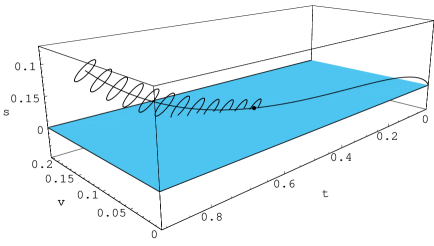
Figure 9: A pictorial representation of density and covariance evolution for the $\text{LDPC}(n,x^{2},x^{5})$. Notice that the ellipsoids corresponding to $(s,t)$ covariances should be regarded as living on a smaller (by a factor $\sqrt{n}$) scale than the typical trajectory.

Those trajectories that hit the $s=0$ plane die. This corresponds to the part of the ellipsoids that vanish.

One can quantify the probability for the process to hit the $s=0$ plane as follows. Stop density and covariance evolution when the number of variables reaches the critical value $v^{*}$. At this point the probability distribution of the state is well approximated by a Gaussian with a given mean and covariance for $s\geq 0$ (while it is obviously 0 for $s<0$). Estimate the survival probability (i.e. the probability of not hitting the $s=0$ plane at any time) by summing the Gaussian distribution over $s\geq 0$. Obviously this integral can be expressed in terms of a $Q$-function.

We will see that the above description leads indeed to the scaling behavior as stated in Lemma 3.1. Where does the shift in Conjecture 3.3 come from? It is easy to understand that we were a bit optimistic (i.e., we underestimated the error probability) in the above calculation: We correctly excluded from the sum the part of the Gaussian distribution lying in the $s<0$ half-space – trajectories contributing to this part must have hit the $s=0$ plane at some point in the past. On the other hand, we cannot be certain that trajectories such that $s>0$ when $v$ crosses $v^{*}$ didn’t hit the $s=0$ plane at some time in the past and bounced back (or will not hit it at some later point). We refer to Section 5 for an in-depth discussion on how to estimate this effect.

Let us finally recall that the performance over the BEC$(\epsilon)$ channel can be easily derived from the results obtained using the model BEC$(n,n\epsilon)$. One can derive the erasure probability for the first case by summing the conditional erasure probability, where the conditioning is on the number of erasures. Notice that the number of erasures for the BEC$(\epsilon)$ is asymptotically Gaussian with mean $n\epsilon$ and standard deviation $\sqrt{n\epsilon\overline{\epsilon}}$. Since this standard deviation is of the same order as the gap to the threshold such a convolution gives a non trivial contribution, unlike in the Shannon ensemble example, cf. Section 1. It is easy to verify that this convolution amounts to computing the parameter $\alpha^{2}$, cf. Lemma 3.1 as the sum of two contributions: one due to the channel fluctuations and the other due to covariance evolution. More precisely we have

$$\alpha_{{\rm BEC}(\epsilon)}^{2}=\alpha_{{\rm BEC}(n,n\epsilon)}^{2}+\epsilon^{*}\overline{\epsilon}^{*}\,,$$ (10)

where we took $\epsilon=\epsilon^{*}$ since we are interested in the region $\epsilon=\epsilon^{*}+O(n^{-1/2})$ and we can neglect $O(n^{-1/2})$ corrections. Hereafter we shall mostly focus on the BEC$(n,n\epsilon)$ channel. The reader is invited to use the formula (10) for translating the results whenever necessary.

3.2 Marginally Stable Ensembles

As already mentioned, marginally stable ensembles are expected to follow a different scaling from the one described in Lemma 3.1. We will limit our discussion to the simplest case, namely the case of cycle code ensembles. We conjecture though that the form of the scaling law is quite general and applies to all marginally stable ensembles. The cycle Poisson ensemble is slightly easier to handle analytically than the standard ensemble. We will therefore formulate our results mainly for this case.

Lemma 3.4.

[Scaling of Block Probability for Cycle Poisson Ensembles] Consider transmission over BEC$(n,n\epsilon)$ using elements from $\text{ELDPC}(n,\lambda(x)=x,r,s)$. Then where $a=\bar{r}^{-1/6}$, $b=\bar{r}^{-2/3}$, $A(s)=\exp\left\{\sum_{s^{\prime}=1}^{s}\frac{1}{2s^{\prime}}\right\}$, and

$$f(x)=\frac{\sqrt{2\pi}3^{2/3}}{2}\,e^{-\frac{4x^{3}}{3}}p(3^{2/3}x;3/2,-1)\,.$$

Hereby, $p(u;\alpha,\beta)$ is a so called stable density with representation

$$p(u;\alpha,\beta)=\frac{1}{2\pi}\int e^{-itu}\,\exp\left\{-|t|^{\alpha}e^{-i\frac{\pi}{2}K(\alpha)\beta{\rm sign}(t)}\right\}\;dt,$$

and $K(\alpha)=1-\mid 1-\alpha\mid$.

Proof 3.5.

In principle one could arrive at the above result by proceeding in the same fashion as for unconditionally stable ensembles, i.e., one could employ the tools of density evolution and covariance evolution.

We will however use an entirely different approach. Note that there is a one-to-one correspondence between elements of $\text{ELDPC}(n,\lambda(x)=x,r,s=2)$ and random graphs on $n\bar{r}$ nodes with exactly $n$ edges, see [20]. If $s=2$, then double edges and cycles of length four are excluded from the Tanner graph. Therefore, each variable node connects two distinct check nodes and no two variable nodes connect the same pair. If we therefore identify each variable node (and the two edges that emanate from it) with one edge in an ordinary graph we get our desired correspondence. Further, the decoder will be successful if and only if this random graph is a forest, i.e., a collection of trees. Let $F(l,k)$ denote the number of forests on $l$ labeled nodes and $k$ components. Such a forest has $l-k$ edges and therefore it corresponds to a constellation on $v=l-k$ variable nodes. Since these variable nodes can be ordered arbitrarily it follows that there are $v!F(n\bar{r},n\bar{r}-v)$ constellations on $v$ variable nodes which do not contain stopping sets.

It remains to find the total number of constellations on $v$ variable nodes which are compatible with the expurgation scheme. The desired result will then follow by diving these two quantities. Assume $s=0$. Then the total number of constellations on $v$ variable nodes is equal to $(n\bar{r})^{2v}$, since for each edge we can choose one of the $n\bar{r}$ check nodes. Let $n_{s}({{\tt G}})$ denote the number of cycles of length $2s$ in a fixed portion of the bipartite graph ${{\tt G}}$ of size $v$. It is easy to verify (and is a well studied problem in random graphs) that $\mathbb{E}[n_{s}({{\tt G}})]=\frac{1}{2s}\left(\frac{2v}{n\bar{r}}\right)^{s}(1+O(1/v))$. Further it is known that for each fixed $s$ the random variables $(n_{1},\cdots n_{s})$ are asymptotically (as $n$ and $v$ tend to infinity with a fixed ratio) independent and follow a Poisson distribution, [4]. Finally, for the Poisson ensemble we have $\epsilon^{*}=\frac{\bar{r}}{2}$ so that around the critical value $v=\epsilon^{*}n=\frac{n\bar{r}}{2}$ and $\frac{2v}{n\bar{r}}=1$. It follows that around the threshold the total number of constellations which are compatible with the expurgation scheme behaves like

$$T(v\sim n\epsilon^{*})=(n\bar{r})^{2v}e^{-\sum_{s^{\prime}=1}^{s}\frac{1}{2s^{\prime}}}(1+O(1/v))=(n\bar{r})^{2v}/A(s)(1+O(1/v)).$$

From this the block error probability around the threshold follows immediately once $F(l,k)$ is known, namely, we have

One of the most celebrated formulas in enumerative combinatorics states that there are $l^{l-2}$ labeled trees on $l$ nodes, [23]. Unfortunately there does not seem to exist an equally elementary expression for the number of labeled forests. The situation is aggravated by the fact that we are interested in the region where the average number of edges per node is around one. Exactly around this region the graph goes through a phase transition and so the behavior of $F(l,k)$ is nontrivial even in the limit of large sizes. Fortunately, the asymptotic behavior has been determined by Britkov [5] and the result has been made accessible (to the English speaking audience) in the book by Kolchin [11]. Our result now follows by employing the asymptotic approximation stated in Theorem 1.4.4 in [11].

Note, that for the cycle case the maximum likelihood and the iterative decoder perform identical in terms of block erasure probability. This is true since in this case the condition of no stopping sets is equal to the condition that there are no cycles which in turns implies that there is no codeword. Note, however, that this is no longer true once we look at the resulting bit erasure probability.

We also note that if we want to get the scaling law for the channel BEC$(\epsilon)$ we need to convolve the above curves with the Binomial with mean $n\epsilon$. However, on the scale $\epsilon^{*}-\epsilon=O(n^{-1/3})$, the effect of the channel fluctuations vanishes in the large blocklength limit. The leading correction to the scaling law (LABEL:BlockScalingCycle) coming from the channel consists in the substitution

$$f(x)\to f(x)+\frac{\epsilon^{*}(1-\epsilon^{*})}{(1-r)^{4/3}}\,f^{\prime\prime}(x)\,n^{-1/3}\,+O(n^{-1/2})\,.$$ (11)

The following lemma characterizes the corresponding limiting block erasure probability curve.

Lemma 3.6.

[Asymptotic Block Erasure Probability Curve] Consider transmission over BEC$(n,n\epsilon)$ or BEC$(\epsilon)$ using random elements from $\text{ELDPC}(n,\lambda(x)=x,r,s)$. Then

$$\lim_{n\rightarrow\infty}$$

The corresponding asymptotic bit erasure probability curve under iterative decoding can be obtained through a standard density evolution analysis and it is given in parametric form by

$$\left(\frac{x}{\lambda(1-\rho(1-x))},\frac{x\Lambda(1-\rho(1-x))}{\lambda(1-\rho(1-x))}\right),$$

where $x\in(x^{*},1]$ and $x^{*}$ is the solution to the equation $\epsilon^{*}\lambda(1-\rho(1-x))=x$. Figure 10 shows the resulting bit and block erasure curves for $\text{ELDPC}(n,\lambda(x)=x,r=\frac{1}{2},s=1)$.

Figure 10: The bit and block erasure probability for $\text{ELDPC}(n,\lambda(x)=x,r=\frac{1}{2},s=1)$ for $n=2^{i}$, $i=8,10,12,14$. As can be seen from the picture, the block erasure curves actually converge to a limiting (non-zero) curve over the whole range of $\epsilon$, whereas the bit erasure curves decrease to zero below the threshold for increasing block lengths. Also shown are the result of using the scaling laws for the block erasure probability as stated in Lemma 3.4.

Cycle codes can not be expurgated up to some linear fraction of the block length since the number of stopping sets of size $s_{1},\cdots s_{k}$ are jointly Poisson and have mean equal to $(2/\bar{r})^{s_{i}}/(2s_{i})$, respectively. Below the threshold $\epsilon^{*}=\bar{r}/2$, the bit erasure probability scales as $1/n$. Expurgation changes uniquely the coefficient of this scaling. A simple calculation yields

where we defined the function

$$L_{s}(x):=\sum_{s^{\prime}=s+1}^{\infty}\frac{x^{s^{\prime}}}{s^{\prime}}=-\log(1-x)-\sum_{s^{\prime}=1}^{s}\frac{x^{s^{\prime}}}{s^{\prime}}\,.$$

As shown in Fig. 11, this formula provides a good approximation to the bit error probability away from the critical region. Notice in fact that the coefficient of the $1/n$ term in Eq. (LABEL:equ:cyclicerrorfloor) diverges as $\epsilon\to\epsilon^{*}$.

Figure 11: Comparison of the exact bit erasure curves (solid line) with the analytic expression given in (LABEL:equ:errorfloor) (dashed lines) for $n=2^{i}$, $i=8,10,12,14$ and $\epsilon<\epsilon^{*}$.

4 Computation of the Variance Parameter

In the previous section we saw that the basic scaling law, cf. Lemma 3.1, only depends on the variance $\alpha^{2}$. In this section we will work out in detail the calculation of this parameter. In Section 5 we will present the method to be used for computing $\beta$ which is needed for the conjectured refined form of the scaling law.

Although conceptually it is straightforward to write down the equations for the general irregular case, the actual computations are quite cumbersome. We will therefore proceed as follows. In Section 4.1 we discuss the covariance evolution equations in an abstract setting. These are applied to particular regular LDPC ensembles in Section 4.2.

4.1 General Covariance Evolution

We regard iterative decoding as a Markov process in a finite dimensional space. The examples in the next two subsections will make clear how this framework can be adapted to particular code ensembles.

Consider a family of Markov chains $X_{n,0},X_{n,1},\dots,X_{n,t},\dots$ parametrized by $n\in{\mathbb{N}}$ and taking values in ${\mathbb{Z}}^{d+1}$. For iterative decoding applications, $n$ will represent the blocklength. We drop the subscript $n$ hereafter. Let the transition probability be and the initial condition be a single non-random state $X_{0}=x_{0}\in{\mathbb{Z}}^{d+1}$. In iterative decoding the initial condition is actually a distribution over states. This case is easy to treat by first conditioning on the initial state, and then convolving with the initial distribution. We will denote the $d+1$ coordinates of the state $x$ as

$$(x^{(0)},x^{(1)},\dots,x^{(d)})=x\in{\mathbb{Z}}^{d+1}\,.$$ (14)

We denote the corresponding random variable by $(X^{(0)},X^{(1)},\dots,X^{(d)})$.

In the following we shall always be interested in times $t<\kappa_{0}\,n$ for a positive constant $\kappa_{0}$ (we reserve the symbols $\kappa_{1},\kappa_{2},\dots$ for numerical constants which we assume not to depend upon $n$). We shall moreover assume the following regularity properties of the Markov chain:

1. The chain makes finite jumps. In other words, there exists a $\kappa_{1}>0$ such that $|X^{(i)}_{t+1}-X^{(i)}_{t}|<\kappa_{1}$ almost surely.

2. The transition probabilities have a smooth $n\to\infty$ limit. In practice there exist functions $\widehat{W}:{\mathbb{Z}}^{d+1}\times{\mathbb{R}}^{d+1}\to{\mathbb{R}}_{+}$ and a positive constant $\kappa_{2}$ such that

   $$|W(\Delta|x)-\widehat{W}(\Delta|x/n)|<\kappa_{2}/n\,.$$ (15)

   Clearly, we have $\sum_{\Delta}\widehat{W}(\Delta|x/n)=1$. We shall moreover assume $\widehat{W}(\Delta|z)$ to be $C^{2}({\mathbb{R}}^{d+1})$ with respect to its second argument and to have bounded first and second derivatives.

3. The process has a finite range on the $n$ scale. In practice, there exists $\kappa_{3}>0$ such that $|X^{(i)}_{t}|<\kappa_{3}\,n$ almost surely.

Under these hypothesis the distribution of $X_{t}$ is well described by a Gaussian whose mean and variance can be obtained by solving some ordinary differential equations. In order to state this fact in a more precise fashion, we need some additional notation. We denote by $\overline{X}_{t}\equiv\mathbb{E}[X_{t}]$ the average of $X_{t}$ and $D^{(ij)}_{t}\equiv\mathbb{E}[X^{(i)}_{t};X^{(j)}_{t}]\equiv\mathbb{E}[X^{(i)}_{t}X^{(j)}_{t}]-\mathbb{E}[X^{(i)}_{t}]\mathbb{E}[X^{(j)}_{t}]$ its covariance. We need furthermore the first two moments of the transition rates $W(\Delta|x)$:

$$f^{(i)}(x) \equiv \sum_{\Delta}\Delta_{i}\,W(\Delta|x)\,,$$ (16)

$$f^{(ij)}(x) \equiv \sum_{\Delta}\Delta_{i}\Delta_{j}\,W(\Delta|x)-f^{(i)}(x)f^{(j)}(x)\,,$$ (17)

with $i,j\in\{0,\dots,d\}$. We shall call $\hat{f}^{(i)}(z)$, $\hat{f}^{(ij)}(z)$ the analogous quantities for the limiting rates $\widehat{W}(\Delta|z)$.

Finally, let $\overline{z}(\tau)\in{\mathbb{R}}^{d+1}$ and $\delta^{(ij)}(\tau)\in{\mathbb{R}}$, for $\tau\in{\mathbb{R}}_{+}$ and $i,j\in\{0,\dots,d\}$, denote the solution of

$$\frac{d\overline{z}^{(i)}}{d\tau}(\tau) = \hat{f}^{(i)}(\overline{z}(\tau))\,,$$ (18)

$$\frac{d\delta^{(ij)}}{d\tau}(\tau) = \hat{f}^{(ij)}(\overline{z}(\tau))+\sum_{k=0}^{d}\left[\delta^{(ik)}(\tau)\left.\frac{\partial\hat{f}^{(j)}}{\partial z^{(k)}}\right|_{\overline{z}(\tau)}+\left.\frac{\partial\hat{f}^{(i)}}{\partial z^{(k)}}\right|_{\overline{z}(\tau)}\delta^{(kj)}(\tau)\right]\,.$$ (19)

with initial conditions $\overline{z}(0)=x_{0}/n$ and $\delta^{(ij)}(0)=0$.

Proposition 4.1.

Under the conditions stated above the following results hold (here we use the symbols $\Omega_{0},\Omega_{1},\dots$, for constants (independent of $n$) which we prove to exist):

1. $X_{t}$ concentrates on the $n$ scale. In formulae, there exist $\Omega_{0}>0$, such that

2. The average and covariance of $X_{t}$ are accurately tracked by $\overline{z}(\tau)$ and $\delta^{(ij)}(\tau)$. More precisely, there exist constants $\Omega_{1},\Omega_{2}>0$, such that

   $$\left|\frac{1}{n}\overline{X}^{(i)}_{t}-\overline{z}^{(i)}(t/n)\right| \leq \frac{\Omega_{1}}{n}\,,$$ (21)

   $$\left|\frac{1}{n}D^{(ij)}_{t}-\delta^{(ij)}(t/n)\right| \leq \frac{\Omega_{2}}{\sqrt{n}}.$$ (22)

3. The variable $(X_{t}-\overline{X}_{t})/\sqrt{n}$ converges weakly to a $(d+1)$-dimensional Gaussian with variance $\delta^{(ij)}(t/n)$. More precisely, define the logarithmic moment generating function

   $$\Lambda_{t}(\lambda)\equiv\log\mathbb{E}\,\exp\left[\frac{1}{\sqrt{n}}\,\,\lambda\cdot(X_{t}-\overline{X}_{t})\right],$$ (23)

   for $\lambda\in{\mathbb{R}}^{d+1}$. Then there exist a function $\lambda\mapsto\Omega_{4}(\lambda)\in{\mathbb{R}}_{+}$, such that

   $$\left|\Lambda_{t}(\lambda)-\frac{1}{2}\sum_{ij}\delta^{(ij)}(t/n)\lambda_{i}\lambda_{j}\right|\leq\frac{\Omega_{4}(\lambda)}{\sqrt{n}}\,.$$ (24)

The proof is quite straightforward and will be outlined in App. A. Here we limit ourselves to a few comments.

Notice that the statements collected in the above proposition are not all independent. Equation (22), may for instance be regarded as a consequence of Eq. (24). The various results are presented in order of increasing sharpness. Also, not all of the assumptions in the points 1-3 are needed to proof each of the statements in the proposition. For instance, the concentration result is an easy consequence of the Hoeffding-Azuma inequality and requires the hypotheses 1 (uniformly bounded jumps), 3 (scaling of time with $n$) plus some Lipschitz property of the drift coefficients $f^{(i)}(x)$, cf. Eq. (16). This point is further discussed in App. A. The limitation to a deterministic initial condition is easily removed. In iterative decoding applications the initial condition is a Gaussian distribution with standard deviation of order $\sqrt{n}$. Convolution with such a distribution amounts to integrating equation (19) and taking as initial condition the initial covariance. Finally, the situation investigated here can be regarded as a discrete analogous of the Friedlin-Wentzell theory of random perturbations of dynamical systems [9].

In the following section we shall apply the above analysis to two LDPC ensembles: the standard regular ensemble $\text{LDPC}(n,x^{{\tt l}-1},x^{{\tt r}-1})$, and the regular Poisson ensemble $\text{LDPC}(n,x^{{\tt l}-1},r)$. The general strategy is the following: $(i)$ Determine a sufficient statistics for the decoding process. For a general $\text{LDPC}(n,\lambda,\rho)$ ensemble, a sufficient statistics is provided by the degree distributions at variable and check nodes in the residual graph. As we will see, a more compact representation is available for the two special cases mentioned above. $(ii)$ Write the transition probability for iterative decoding and compute the drift and diffusion coefficients, cf. Eqs. (16), (17). $(iii)$ Determine the initial condition, namely the average state, and its variance before the decoding process has been started. $(iv)$ Integrate the density evolution and covariance evolution equation, cf. Eq. (18) and (19) up to the critical point. The parameter $\alpha$ in Lemma 3.1 is finally given (up to a rescaling) by the standard deviation of the number of degree one check nodes $s$ at the critical point. More precisely:

$$\alpha=\sqrt{\delta_{\sigma\sigma}}\left(\frac{\partial\sigma}{\partial\epsilon}\right)^{-1}\,,$$ (25)

both factors being evaluated at the critical point.

4.2 Regular Ensembles

We will now show the explicit computations that need to be done in order to accomplish the program outlined in the previous section for the case of regular standard and Poisson ensembles.

There are some significant simplifications that arise in this case. Note that the triple $(v,s,t)$ constitutes a sufficient statistics, i.e., it suffices to keep track of the number of variable nodes (all of which have degree ${\tt l}$ since by assumption the graph is regular), the number of degree-one check nodes and the number of check nodes of degree two or higher. This can be seen as follows. We claim that all constellations of “type” $(v,s,t)$ have uniform probability. To see this let $\tilde{{{\tt G}}}_{1}$ and $\tilde{{{\tt G}}}_{2}$ be two residual graphs of type $(v,s,t)$. Assume that $\tilde{{{\tt G}}}_{1}$ is the result of applying the iterative decoder to the graph ${{\tt G}}_{1}$ with a particular channel realization and a particular sequence of choices of the iterative decoder. It is then easy to see that there exists a graph ${{\tt G}}_{2}$ which differs from ${{\tt G}}_{1}$ only on the residual part (where it coincides with $\tilde{{{\tt G}}}_{2}$) but agrees with it otherwise. By definition of the ensemble, ${{\tt G}}_{1}$ and ${{\tt G}}_{2}$ have equal probability and if the iterative decoder is applied to ${{\tt G}}_{2}$ with the same channel realization and sequence of random choices we get $\tilde{{{\tt G}}}_{2}$. This shows that $\tilde{{{\tt G}}}_{1}$ and $\tilde{{{\tt G}}}_{2}$ (and therefore any residual graph which is compatible with the degree distribution) have equal probability. It follows that, given $(v,s,t)$, the distribution of ${{\tt G}}$ is determined so that $(v,s,t)$ indeed constitutes a state.

Let us now determine the degree distribution of a “typical” element ${{\tt G}}$ of type $(v,s,t)$, since this knowledge will be required in the sequel. For the standard ensemble define the generator polynomial $p(z):=(1+z)^{{\tt r}}-{\tt r}z-1$ which counts the number of connections into a check node of degree two or higher. For the Poisson ensemble the equivalent function is $p(z):=e^{z}-z-1$. Define $a(z):=z\frac{p^{\prime}(z)}{p(z)}$. The total number of constellations on $t$ check nodes of degree at least two with $v{\tt l}-s$ edges is easily seen to be $\text{coef}\left\{p(x)^{t},x^{v{\tt l}-s}\right\}$. Let $t_{i}$, $i\geq 2$, denote the number of check nodes of degree $i$. Then the total number of constellations which are compatible with the desired type can be written as

$$\sum_{t_{2},t_{3},\cdots:\sum_{i\geq 2}t_{i}=t;\sum_{i\geq 2}it_{i}=v{\tt l}-s}\binom{t}{t_{2},t_{3},\cdots}\left(\prod_{i\geq 2}p_{i}^{t_{i}}\right).$$

Since all constellations have equal probability a “typical” constellation will have the type which “dominates” the above sum. Some calculus reveals that this dominating type has the form

$$\tau_{i}=\frac{p_{i}z^{i}}{p(z)}\tau\,,\;\;\;\;\;\;i\geq 2,$$ (26)

where $\tau_{i}$, $i\geq 2$, denotes the fraction of check nodes of degree $i$ and where $a(z)=\frac{\nu{\tt l}-\sigma}{\tau}$.

We will see shortly that for the Poisson case it suffices to consider ensembles of rate zero since the scaling parameters for the general case can be easily connected to this case. Therefore in the next theorem we can assume without loss of generality that the rate is zero for Poisson ensembles.

Lemma 4.2.

[Drift, Variance and Partial Derivatives for Regular Ensembles] Consider regular standard ensembles $\text{LDPC}(n,x^{{\tt l}-1},x^{{\tt r}-1})$ or regular Poisson ensembles $\text{LDPC}(n,x^{{\tt l}-1},r=0)$. Define

$$p(z) = \begin{cases}(1+z)^{{\tt r}}-1-{\tt r}z,&\text{standard ensemble},\\ e^{z}-1-z,&\text{Poisson ensemble},\end{cases}$$

and let $a(z):=z\frac{p^{\prime}(z)}{p(z)}$. Let $x_{l}$ denote the right-to-left erasure probability and let $x_{r}:=\epsilon\lambda(x_{l})$. Then along the density evolution path parametrized by $x_{l}$ we have

$$\hat{f}^{(\tau)} =-({\tt l}-1)\frac{2\tau_{2}}{\nu{\tt l}}, \hat{f}^{(\sigma)} =-1-({\tt l}-1)\frac{\sigma}{\nu{\tt l}}-\hat{f}^{(\tau)},$$

$$\hat{f}^{(\tau\tau)} =-\hat{f}^{(\tau)}\left(1+\frac{\hat{f}^{(\tau)}}{{\tt l}-1}\right), \hat{f}^{(\sigma\tau)} =\hat{f}^{(\tau)}\left(1-\frac{\hat{f}^{(\sigma)}+1}{{\tt l}-1}\right)\,,$$

$$\frac{\partial\hat{f}^{(\tau)}}{\partial\sigma} =\frac{2({\tt l}-1)}{\nu{\tt l}}\frac{p_{2}z(2-a(z))}{a^{\prime}(z)p(z)}, \frac{\partial\hat{f}^{(\sigma)}}{\partial\nu} =\frac{{\tt l}-1}{\nu{\tt l}}\frac{\sigma}{\nu}-\frac{\partial\hat{f}^{(\tau)}}{\partial\nu}$$

$$\frac{\partial\hat{f}^{(\sigma)}}{\partial\tau} =-\frac{\partial\hat{f}^{(\tau)}}{\partial\tau}, \frac{\partial\hat{f}^{(\sigma)}}{\partial\sigma} =-\frac{{\tt l}-1}{\nu{\tt l}}-\frac{\partial\hat{f}^{(\tau)}}{\partial\sigma},$$

$$\hat{f}^{(\sigma\sigma)} = -\frac{\left(\hat{f}^{(\tau)}\right)^{2}}{{\tt l}-1}-({\tt l}-1)\left(\frac{\sigma}{\nu{\tt l}}-1\right)\frac{\sigma}{\nu{\tt l}}-\hat{f}^{(\tau)}\left(1+2\frac{\sigma}{\nu{\tt l}}\right),$$

$$\frac{\partial\hat{f}^{(\tau)}}{\partial\nu} = -\frac{2({\tt l}-1)}{\nu{\tt l}}\left(-\frac{\tau_{2}}{\nu}+\frac{p_{2}z{\tt l}(2-a(z))}{a^{\prime}(z)p(z)}\right)$$

$$\frac{\partial\hat{f}^{(\tau)}}{\partial\tau} = -\frac{2({\tt l}-1)}{\nu{\tt l}}\left(\frac{\tau_{2}}{\tau}-\frac{p_{2}za(z)(2-a(z))}{a^{\prime}(z)p(z)}\right),$$

where for the standard regular ensemble $z=\frac{\epsilon\lambda(x_{l})}{1-\epsilon\lambda(x_{l})}$ whereas for the Poisson regular ensemble $z=\frac{\epsilon\lambda(x_{l})}{\int\lambda}$.

Proof 4.3.

Let $\sigma$ denote the fraction of degree-one check nodes, $\tau_{i}$, $i\geq 2$, the fraction of degree-$i$ check nodes and $\nu$ denote the fraction of residual variable nodes. Since the total edge count on the left and right must match up we have $\sigma+\sum_{i=2}i\tau_{i}=\nu{\tt l}$. A random edge therefore has probability $q_{1}:=\frac{\sigma}{\nu{\tt l}}$ of being connected to a degree-one check node and probability $q_{i}:=\frac{i\tau_{i}}{\nu{\tt l}}$ of being connected to a degree-$i$ check node, $i\geq 2$. For large $n$, the joint probability distribution of all ${\tt l}$ edges emanating from a variable node converges to the product distribution. It follows that (in this large blocklength limit) the probability distribution (for a randomly chosen variable node) of having $u_{1}$ connections into degree-one check nodes and $u_{2}$ connections into degree-two check nodes is given by

$$\tilde{w}(u_{1},u_{2}):=\binom{{\tt l}}{u_{1},u_{2},{\tt l}-u_{1}-u_{2}}q_{1}^{u_{1}}q_{2}^{u_{2}}(1-q_{1}-q_{2})^{{\tt l}-u_{1}-u_{2}}.$$

In the iterative decoding process variables are not picked at random though. A variable node is picked with a probability which is proportional to $u_{1}$. Therefore, the induced probability distribution under iterative decoding is

$$w(u_{1},u_{2})=\frac{\tilde{w}(u_{1},u_{2})u_{1}}{\sum_{u_{1}^{\prime},u_{2}^{\prime}}\tilde{w}(u_{1}^{\prime},u_{2}^{\prime})u_{1}^{\prime}}=\tilde{w}(u_{1},u_{2})\frac{u_{1}}{{\tt l}q_{1}}\,,$$ (27)

Note that the generating function of $w(u,v)$ has the compact description

$$W(x,y) := \sum_{u_{1},u_{2}}w(u_{1},u_{2})x^{u_{1}}y^{u_{2}}=x(xq_{1}+yq_{2}+(1-q_{1}-q_{2}))^{{\tt l}-1}.$$

In terms of $W(x,y)$ we have

$$\hat{f}^{(\tau)} = -\sum_{u_{1},u_{2}}w(u_{1},u_{2})u_{2}=-\left.\frac{\partial W(x,y)}{\partial y}\right|_{x=y=1}$$

$$= -({\tt l}-1)q_{2}=-({\tt l}-1)\frac{2\tau_{2}}{\nu{\tt l}},$$

$$\hat{f}^{(\sigma)} = -\sum_{u_{1},u_{2}}w(u_{1},u_{2})(u_{1}-u_{2})=-\left.\frac{\partial W(x,y)}{\partial x}\right|_{x=y=1}-\hat{f}^{(\tau)}$$

$$= -1-({\tt l}-1)q_{1}-\hat{f}^{(\tau)}=-1-({\tt l}-1)\frac{\sigma}{\nu{\tt l}}-\hat{f}^{(\tau)},$$

$$\hat{f}^{(\tau\tau)} = \sum_{u_{1},u_{2}}w(u_{1},u_{2})u_{2}^{2}-\left(\hat{f}^{(\tau)}\right)^{2}=\left.\frac{\partial^{2}W(x,y)}{\partial y^{2}}\right|_{x=y=1}-\hat{f}^{(\tau)}-\left(\hat{f}^{(\tau)}\right)^{2}$$

$$= ({\tt l}-1)({\tt l}-2)q_{2}^{2}-\hat{f}^{(\tau)}-\left(\hat{f}^{(\tau)}\right)^{2}=-\hat{f}^{(\tau)}\left(1+\frac{\hat{f}^{(\tau)}}{{\tt l}-1}\right),$$

$$\hat{f}^{(\sigma\tau)} = \sum_{u,v}w(u_{1},u_{2})(u_{1}-u_{2})u_{2}-\hat{f}^{(\sigma)}\hat{f}^{(\tau)}=\left.\frac{\partial^{2}W(x,y)}{\partial xy}\right|_{x=y=1}-\hat{f}^{(\tau\tau)}-\left(\hat{f}^{(\tau)}\right)^{2}-\hat{f}^{(\sigma)}\hat{f}^{(\tau)}$$

$$= -\hat{f}^{(\tau)}(1+({\tt l}-2)q_{1})-\hat{f}^{(\tau\tau)}-\left(\hat{f}^{(\tau)}\right)^{2}-\hat{f}^{(\sigma)}\hat{f}^{(\tau)}=\hat{f}^{(\tau)}\left(1-\frac{\hat{f}^{(\sigma)}+1}{{\tt l}-1}\right)$$

$$\hat{f}^{(\sigma\sigma)} = \sum_{u_{1},u_{2}}w(u_{1},u_{2})(u_{1}-u_{2})^{2}-\left(\hat{f}^{(\sigma)}\right)^{2}$$

$$= \left.\frac{\partial^{2}W(x,y)}{\partial x^{2}}\right|_{x=y=1}-\hat{f}^{(\sigma\tau)}-\hat{f}^{(\sigma)}\hat{f}^{(\tau)}-\hat{f}^{(\tau\tau)}-\left(\hat{f}^{(\tau)}\right)^{2}-\hat{f}^{(\sigma)}-\hat{f}^{(\tau)}-\left(\hat{f}^{(\sigma)}\right)^{2}$$

$$= ({\tt l}-1)q_{1}\left(2+({\tt l}-2)q_{1}\right)-\hat{f}^{(\sigma\tau)}-\hat{f}^{(\sigma)}\hat{f}^{(\tau)}-\hat{f}^{(\tau\tau)}-\left(\hat{f}^{(\tau)}\right)^{2}-\hat{f}^{(\sigma)}-\hat{f}^{(\tau)}-\left(\hat{f}^{(\sigma)}\right)^{2}$$

$$= -\frac{\left(\hat{f}^{(\tau)}\right)^{2}}{{\tt l}-1}-({\tt l}-1)\left(\frac{\sigma}{\nu{\tt l}}-1\right)\frac{\sigma}{\nu{\tt l}}-\hat{f}^{(\tau)}\left(1+2\frac{\sigma}{\nu{\tt l}}\right).$$

Next we need to determine the partial derivatives. From equation (26) for $i=2$ we have

$$\frac{\partial\hat{f}^{(\tau)}}{\partial\tau} = -\frac{2({\tt l}-1)}{\nu{\tt l}}\frac{\partial\tau_{2}}{\partial\tau}=-\frac{2({\tt l}-1)}{\nu{\tt l}}\left(\frac{\tau_{2}}{\tau}+\tau\frac{\partial p_{2}\frac{z^{2}}{p(z)}}{\partial z}\frac{\partial z}{\partial\tau}\right)$$

$$= -\frac{2({\tt l}-1)}{\nu{\tt l}}\left(\frac{\tau_{2}}{\tau}-\frac{p_{2}za(z)(2-a(z))}{a^{\prime}(z)p(z)}\right).$$

The remaining derivatives follow in the same way and we skip the details. Now note that along the typical decoding trajectory all quantities required to compute the above expressions are given by the density evolution equations (6) and (7).

It remains to establish the link between $z$ and $x_{l}$. We start with standard ensembles. From the density evolution equation (7)

$$\tau_{2} = \frac{\binom{{\tt r}}{2}x_{r}^{2}(1-x_{r})^{{\tt r}-2}}{\sum_{i\geq 2}\binom{{\tt r}}{i}x_{r}^{i}(1-x_{r})^{{\tt r}-i}}\tau=\frac{\binom{{\tt r}}{2}\left(\frac{x_{r}}{1-x_{r}}\right)^{2}}{\sum_{i\geq 2}\binom{{\tt r}}{i}\left(\frac{x_{r}}{1-x_{r}}\right)^{i}}\tau=\frac{p_{2}\left(\frac{x_{r}}{1-x_{r}}\right)^{2}}{p\left(\frac{x_{r}}{1-x_{r}}\right)}\tau.$$

Comparing this to equation (26) it follows that $z=\frac{x_{r}}{1-x_{r}}=\frac{\epsilon\lambda(x_{l})}{1-\epsilon\lambda(x_{l})}$.

Recall that in the Poisson case we can assume that $r=0$, so that $\rho(x)=R(x)=e^{\frac{x-1}{\int\lambda}}$. Again from (7)

$$\tau_{2} = \frac{x_{r}^{2}}{2(\int\lambda)^{2}}R(1-x_{r})=\frac{p_{2}\left(\frac{x_{r}}{\int\lambda}\right)^{2}}{p\left(\frac{x_{r}}{\int\lambda}\right)}\tau,$$

from which it follows that for the Poisson case

$$z=\frac{\epsilon\lambda(x_{l})}{\int\lambda}.$$

Figure 12 depicts $\hat{f}^{(\sigma\sigma)}$, $\hat{f}^{(\sigma\tau)}$ and $\hat{f}^{(\tau\tau)}$ as a function of $\nu$ along the critical trajectory (i.e., for the choice $\epsilon=\epsilon^{*}\approx 0.4294$) for the $\text{LDPC}(n,x^{2},x^{5})$ ensemble.

Figure 12: The evolution of $\hat{f}^{(\sigma\sigma)}$ (dashed line), $\hat{f}^{(\sigma\tau)}$ (dotted line) and $\hat{f}^{(\tau\tau)}$ (solid line) along the critical trajectory for the $\text{LDPC}(n,x^{2},x^{5})$ ensemble.

The last piece of information required to apply the strategy outlined in the previous subsection, consists in determining the initial condition for the density and covariance evolution. This is provided by the following lemmas, whose proof are fairly routine and therefore left to the reader.

Lemma 4.4.

[Initial Condition for Standard Regular Ensembles] Consider transmission over the channel BEC$(n,n\epsilon)$ using a random element of $\text{LDPC}(n,x^{{\tt l}-1},x^{{\tt r}-1})$. Consider the residual graph (after reception of the transmitted word) and let denote the distribution of check nodes of degree one and of degree at least two, respectively. Then

where is a (discrete) Gaussian density with mean

$$\frac{1}{n}\mathbb{E}[s] = {\tt l}\epsilon(1-\epsilon)^{{\tt r}-1}\,,$$

$$\frac{1}{n}\mathbb{E}[t] = \frac{{\tt l}}{{\tt r}}\left(1-(1-\epsilon)^{{\tt r}}-{\tt r}\epsilon(1-\epsilon)^{{\tt r}-1}\right)\,,$$

and covariance

$$\frac{1}{n}\mathbb{E}[s;s] = {\tt l}\epsilon\bar{\epsilon}^{{\tt r}-1}(1-\bar{\epsilon}^{{\tt r}-2}(1+\epsilon(({\tt r}-1)\epsilon-1){\tt r}))\,,$$

$$\frac{1}{n}\mathbb{E}[s;t] = -{\tt l}\epsilon\bar{\epsilon}^{{\tt r}-1}(1-\bar{\epsilon}^{{\tt r}-2}(1+\epsilon(({\tt r}-1)^{2}\epsilon-1))),$$

$$\frac{1}{n}\mathbb{E}[t;t] = \frac{{\tt l}\bar{\epsilon}^{{\tt r}-1}}{{\tt r}}(1+({\tt r}-1)\epsilon-\bar{\epsilon}^{{\tt r}-2}(1+\epsilon(2{\tt r}-3+({\tt r}-3)({\tt r}-1)\epsilon+({\tt r}-1)^{3}\epsilon^{2})))\,.$$

Lemma 4.5.

[Initial Condition for Regular Poisson Ensemble] A statement analogous to Lemma 4.4 holds in the case of Poisson ensembles. For $r=0$ the distribution of $s$ and $t$ is again a (discrete) Gaussian with mean

$$\frac{1}{n}\mathbb{E}[s] = {\tt l}\epsilon\;e^{-{\tt l}\epsilon}\,,$$

$$\frac{1}{n}\mathbb{E}[t] = 1-e^{-{\tt l}\epsilon}-{\tt l}\epsilon\;e^{-{\tt l}\epsilon}\,,$$

and covariance

$$\frac{1}{n}\mathbb{E}[s;s] = {\tt l}\epsilon\;e^{-{\tt l}\epsilon}-{\tt l}\epsilon(1-{\tt l}\epsilon+{\tt l}^{2}\epsilon^{2})\;e^{-2{\tt l}\epsilon}\,,$$

$$\frac{1}{n}\mathbb{E}[s;t] = -{\tt l}\epsilon\;e^{-{\tt l}\epsilon}+{\tt l}\epsilon(1+{\tt l}^{2}\epsilon^{2})\;e^{-2{\tt l}\epsilon}\,,$$

$$\frac{1}{n}\mathbb{E}[t;t] = (1+{\tt l}\epsilon)\,e^{-{\tt l}\epsilon}-(1+2{\tt l}\epsilon+{\tt l}^{2}\epsilon^{2}+{\tt l}^{3}\epsilon^{3})\,e^{-2{\tt l}\epsilon}\;\,.$$

Note that, as one would expect, the random variables $(s,t)$ are in general correlated.

We can now solve equations (18) and (19). This allows us to track the evolution of the probability distribution of $s$ and $t$ as $v$ decreases from $n\epsilon$ to $0$, assuming that the $s=0$ plane was not hit earlier.

Example 4.6.

[$(3,6)$-Ensemble] Figure 13 shows the evolution of $\delta^{(ss)}$, $\delta^{(st)}$, $\delta^{(tt)}$ for the $\text{LDPC}(n,x^{2},x^{5})$ ensemble for the choice $\epsilon=\epsilon^{*}\approx 0.42944$. Notice that the variances of $s$ and $t$ can actually shrink as the decoding process evolves. This is an effect of the term in square brackets in equation (19). In particular the variance shrinks to 0 at $\nu=0$ if $\epsilon$ is low enough (whenever decoding is successful with high probability).

Figure 13: The evolution of $\delta^{(ss)}$ (dashed line), $\delta^{(st)}$ (dotted line) and $\delta^{(tt)}$ (solid line) for the $\text{LDPC}(n,x^{2},x^{5})$ ensemble and the choice $\epsilon=\epsilon^{*}\approx 0.42944$.

Finally, the parameter $\alpha$ is given by equation (25), where the first factor can be computed as in equation (9).

In Table (1) we report the values of $\epsilon^{*}$, $\alpha$, and $\beta$ for a few regular standard ensembles. Further explanations concerning the parameter $\beta$ are provided in Section 5.

${\tt l}$	${\tt r}$	$\epsilon^{*}$	$\alpha$	$\beta/\Omega$
3	4	$0.6473$	$0.260115$	$0.593632$
3	5	$0.5176$	$0.263814$	$0.616196$
3	6	$0.4294$	$0.249869$	$0.616949$
4	5	$0.6001$	$0.241125$	$0.571617$
4	6	$0.5061$	$0.246776$	$0.574356$
5	6	$0.5510$	$0.228362$	$0.559688$
6	7	$0.5079$	$0.280781$	$0.547797$
6	12	$0.3075$	$0.170218$	$0.506326$

Table 1: Thresholds and scaling parameters for some regular standard ensembles. The shift parameter is given as $\beta/\Omega$ where $\Omega$ is the universal constant stated in equation (46) whose numerical value is very close to 1.

The computation of the scaling parameters $\alpha=\alpha({\tt l},r)$ and $\beta=\beta({\tt l},r)$ for the Poisson case are made easier by the following pleasing relationship.

Lemma 4.7.

[Scaling of Erasure Probability for Poisson Ensembles] Consider transmission over BEC$(n,n\epsilon)$ using elements from the regular Poisson ensemble $\text{LDPC}(n,x^{{\tt l}-1},r)$. For ${\tt l}$ fixed and $(n,r,\epsilon)$ and $(n^{\prime},r^{\prime},\epsilon^{\prime})$ such that $n\epsilon=n^{\prime}\epsilon^{\prime}$ and $(1-r)n=(1-r^{\prime})n^{\prime}$,

$$\mathbb{E}_{\text{LDPC}(n,x^{{\tt l}-1},r)}[ =\mathbb{E}_{\text{LDPC}(n^{\prime},x^{{\tt l}-1},r^{\prime})}[$$

$$n\mathbb{E}_{\text{LDPC}(n,x^{{\tt l}-1},r)}[ =n^{\prime}\mathbb{E}_{\text{LDPC}(n^{\prime},x^{{\tt l}-1},r^{\prime})}[$$

Proof 4.8.

We start with the statement regarding the block erasure probability. Compare transmission over BEC$(n,n\epsilon)$ using elements from $\text{LDPC}(n,x^{{\tt l}-1},r)$ to transmission over BEC$(n^{\prime},n^{\prime}\epsilon^{\prime})$ using elements from $\text{LDPC}(n^{\prime},x^{{\tt l}-1},r^{\prime})$. The condition $n\epsilon=n^{\prime}\epsilon^{\prime}$ implies that the number of erased bits is the same in both cases. Decoding fails if these erased bits contain a stopping set. The condition $(1-r)n=(1-r^{\prime})n^{\prime}$ implies that the two ensembles have the same number of check nodes. Together with the fact that ${\tt l}$ is the same in both cases (and therefore the involved number of edges is the same) this shows that the erasure probability is the same.

The proof regarding the bit erasure probability is almost identical. Both decoders get stuck in identical constellations. The factor $n$ takes into account what fraction of the overall codeword this constellation is.

If we combine the above relationship with the general form of the scaling law, cf. equations (2) and (3) as well as Lemma 3.1, we get the following scaling relations.

Lemma 4.9.

[Scaling of Scaling Parameters] Consider transmission over BEC$(n,n\epsilon)$ using elements of the Poisson ensemble $\text{LDPC}(n,x^{{\tt l}-1},r)$ with threshold $\epsilon^{*}({\tt l},r)$. Assume that the scaling (3) holds and let $\alpha({\tt l},r)$ and $\beta({\tt l},r)$ denote the corresponding variance and shift parameters. Then

$$\epsilon^{*}({\tt l},r^{\prime}) = \epsilon^{*}({\tt l},r)\,\frac{1-r^{\prime}}{1-r}\,,$$ (28)

$$\alpha({\tt l},r^{\prime}) = \alpha({\tt l},r)\,\left(\frac{1-r^{\prime}}{1-r}\right)^{1/2}\,,$$ (29)

$$\beta({\tt l},r^{\prime}) = \beta({\tt l},r)\,\left(\frac{1-r^{\prime}}{1-r}\right)^{1/3}\,.$$ (30)

Proof 4.10.

The proof is elementary and we leave it to the reader. We note that in order to prove (28) and (29) only the simplified form of the scaling law (2) is required as hypothesis and that this scaling law is proved in Lemma 3.1.

From the above observations it follows that we have to determine the parameters $\epsilon^{*}({\tt l},r)$, $\alpha({\tt l},r)$ and $\beta({\tt l},r)$ only for one rate $r$. This is the reason why so far we have only considered Poisson ensembles of zero rate. Our results will depend only on ${\tt l}$. Relations (28)-(30) can be used to reintroduce the dependence upon $r$.

${\tt l}$	$\epsilon^{*}$	$\alpha$	$\beta/\Omega$
3	$0.818469$	$0.497867$	$0.964528$
4	$0.772280$	$0.409321$	$0.827849$
5	$0.701780$	$0.375892$	$0.760593$
6	$0.637081$	$0.354574$	$0.713490$
7	$0.581775$	$0.337788$	$0.676647$
8	$0.534997$	$0.323501$	$0.646335$
9	$0.495255$	$0.310948$	$0.620646$
10	$0.461197$	$0.299739$	$0.598429$

Table 2: Thresholds and scaling parameters for some Poisson ensembles $\text{LDPC}(n,x^{{\tt l}-1},r)$. Note that these parameters assume that $r=0$. Parameters for a generic rate can be obtained from these parameters through equations. (28)-(30). The shift parameter is given as $\beta/\Omega$ where $\Omega$ is the universal constant stated in (46) whose numerical value is very close to 1.

5 Computation of the Shift Parameter

In this section we explain in greater detail the arguments for Conjecture 3.3, and the procedure for computing the shift parameter $\beta$. As in the previous section, we shall first discuss this issue in an abstract setting, cf. Section 5.1. The general procedure will then be applied to regular standard and Poisson ensembles in Section 5.2.

5.1 The General Approach

Let us reconsider the setting of Section 4.1, i.e., a family of Markov chains $X_{n,0},X_{n,1},\dots,X_{n,t},\dots$ taking values in ${\mathbb{Z}}^{d+1}$ and parametrized by the (large) integer $n$. As before we will drop in the sequel the subscript $n$ to mitigate the notational burden. Throughout this section we shall assume the hypotheses of Proposition 4.1 to be fulfilled. Unlike in Section 4.1, we are interested in paths $X_{0}^{t}\equiv\{X_{0},X_{1},\dots,X_{t}\}$ which are confined to the ‘half space’:

$${\mathbb{H}}_{+}\equiv\{x=(x^{(0)},\dots,x^{(d)})\in{\mathbb{Z}}^{d+1}:\;\;x^{(0)}>0\}\,.$$ (31)

We would like to estimate the ‘survival’ probability

$$P_{t}\equiv$$ (32)

Notice that $P_{t}$ depends implicitly on the initial condition $X_{0}=x_{0}\in{\mathbb{H}}_{+}$. The coordinate $X^{(0)}_{t}$ should be thought as (an abstraction of) the number $s$ of degree-one check nodes in the analysis of iterative decoding, cf. Section 3. The survival probability $P_{t}$ is therefore the probability of not having encountered a stopping set after $t$ steps of the decoding process. We are interested in a time window of length $O(n)$. Without loss of generality we may fix $\tau_{\rm max}>0$ and consider $t\in\{0,\dots,t_{\rm max}\}$ with $t_{\rm max}=\lfloor n\tau_{\rm max}\rfloor$.

We shall denote by $\overline{z}(\tau)$ the ‘critical trajectory’, i.e. a solution of the density evolution equations (18), such that $\overline{z}^{(0)}(\tau^{*})=0$, and $\overline{z}^{(0)}(\tau)>0$ for any $\tau\in[0,\tau_{\rm max}]$, $\tau\neq\tau^{*}$. We call $z_{0}=\overline{z}(0)$ the corresponding initial condition. In order to make contact with the application to iterative decoding, we shall make the following assumptions.

1. As $n\to\infty$, we have $x_{0}=n\,z_{0}+\sqrt{n}\,z_{1}+O(1)$, with $z_{1}\in{\mathbb{R}}^{d+1}$ independent of $n$. This corresponds to the erasure probability $\epsilon$ being in the critical window $\epsilon^{*}-\epsilon=O(n^{-1/2})$.

2. Let $\overline{z}_{u}(\tau)$, $u\in{\mathbb{R}}^{d+1}$, be a ‘perturbed’ critical trajectory obtained by solving the density evolution equations (18) with initial condition $\overline{z}_{u}(\tau^{*})=\overline{z}(\tau^{*})+u$. As for the critical trajectory, we consider this solution in the interval $[0,\tau_{\rm max}]$ and take $u$ such that $|u|<\varepsilon$ with $\varepsilon$ small enough. We assume that there exist a positive $u$-independent constant $\kappa_{1}$, and a function $u\mapsto a(u)$ such that

   $$\overline{z}^{(0)}_{u}(\tau)-\overline{z}^{(0)}_{u}(\tau^{*})\geq a(u)(\tau-\tau^{*})+\kappa_{1}(\tau-\tau^{*})^{2}$$

   for any $\tau\in[0,\tau_{\max}]$.

3. We finally assume that $a(u)$ can be chosen in such a way that $|a(u)|<\kappa_{2}|u|$ for some positive constant $\kappa_{2}$.

Notice that the assumptions B and C above can be easily checked on the ‘continuum’ transition rates $\widehat{W}(\Delta|z)$ introduced in Sec. 4.1. The situation considered here mimics the one found in iterative decoding of unconditionally stable ensembles.

Consider the survival probability $P_{t_{\rm max}}$ at the ‘latest’ time. As we have seen in Section 4.1, most of the trajectories $X_{0}^{t_{\rm max}}$ are concentrated within $\sqrt{n}$ around $n\overline{z}(t/n)$. Therefore the absolute minimum of $X_{t}^{(0)}$ in the interval $\{0,\dots,t_{\rm max}\}$ will be realized for a $t$ ‘close’ to $n\tau^{*}$. If this absolute minimum is positive, the corresponding trajectory contributes to $P_{t_{\rm max}}$, otherwise it does not.

In order to formalize this argument, fix $t^{*}=\lfloor n\tau^{*}\rfloor$. Then

$$P_{t_{\rm max}}=\sum_{x\in{\mathbb{H}}_{+}\ }$$ (33)

Thanks to Proposition 4.1 we can accurately estimate the factor . The term is the probability that the global minimum of $X^{(0)}_{t}$, $t\in\{0\dots t_{\rm max}\}$, is positive conditioned on $X_{t^{*}}=x$.

Figure 14: A pictorial view of decoding trajectories near the critical point. The type of trajectory depicted here is responsible for the shift appearing in the refined scaling form (3).

Let us denote by $t_{\rm g}$ a ‘time’ for which the global minimum is realized. More precisely, $t_{\rm g}\in\{0\dots t_{\rm max}\}$ is a random variable such that $X^{(0)}_{t_{\rm g}}\leq X^{(0)}_{t}$ for all $t\in\{0\dots t_{\rm max}\}$. Call $\overline{z}_{X}(\tau)$ the perturbed critical trajectory defined above with perturbation vector $u=X_{t^{*}}/n-\overline{z}(\tau^{*})$. In other words, we perturbe the critical trajectory by an $O(1/\sqrt{n})$ amount in order to match it to the particular (finite $n$) realization of the Markov process we are dealing with within the critical region. Concentration arguments, analogous to the ones used to prove the point I of Proposition 4.1, imply that, for a given $t$: for some positive constants $\Omega_{1}$ and $\Omega_{2}$ (as before we use this symbols to denote generic constants which are proven to exist independent of $n$). In fact a stronger condition holds true: by Doob’s maximal inequality [16, p. 227], for $T$ fixed for some (possibly different) constants $\Omega_{1}$ and $\Omega_{2}$. Using this fact we can prove an useful result:

Lemma 5.1.

Assume the same hypotheses as in Lemma 4.1 plus A, B and C above. Let $t_{\rm g}$ be a time at which the absolute minimum of $X^{(0)}_{t}$ is realized, for $t\in\{0\dots t_{\rm max}\}$. Then there exist positive constants $\Omega_{1}$, $\Omega_{2}$ and $\delta_{0}$, and a function $n_{0}(\delta)$ such that, for any $\delta>\delta_{0}$ and $n>n_{0}(\delta)$

The proof is deferred to Appendix C. The content of this lemma is illustrated in Fig. 14.

The above result implies that corrections to the simplified scaling of Lemma 3.1 can be estimated through a two step procedure. In a nutshell: $(i)$ Compute the probability for $X_{t^{*}}^{(0)}$ to be of order $n^{1/3}$; $(ii)$ Evaluate the probability for $X^{(0)}_{t_{\rm g}}$ to be positive, conditioned on a given $X_{t^{*}}^{(0)}$ of order $n^{1/3}$.

5.1.1 Distribution of $X_{t^{*}}$

The simplified scaling form, cf. Lemma 3.1, was obtained by approximating the first factor in equation (LABEL:eq:SurvivalRepresentation) by 1. The leading correction to this approximation comes from trajectories such that $X_{t^{*}}^{(0)}=O(n^{1/3})$. Because of Proposition 4.1, the probability distribution of $X_{t^{*}}^{(0)}$ (second factor) is well approximated by a Gaussian with center at $O(\sqrt{n})$ and variance of order $n$. The probability of having $X_{t^{*}}^{(0)}=O(n^{1/3})$ is therefore of order $n^{1/3}\cdot n^{-1/2}=n^{-1/6}$. This explains why the correction term in the refined scaling form (3) is of order $n^{-1/6}$.

This argument can be made more precise by rewriting equation (LABEL:eq:SurvivalRepresentation) as

$$P_{t_{\rm max}}=$$ (36)

The first term corresponds to the simplified scaling form. We shall hereafter focus on the second one, $P_{\rm corr}\equiv$. Notice that varies much more rapidly (on a scale of order $n^{1/3}$) in $x^{(0)}$ than in the other coordinates (on a scale of order $n$). It is therefore useful to introduce the notation $\vec{x}=(x^{(1)}\dots x^{(d)})$ (and analogously $\vec{X}$ and $\vec{z}$) which distinguish explicitly the last $d$ coordinates of $x$. Since varies on a scale $n^{1/2}$, we can safely approximate it by setting the coordinate $x^{(0)}$ to 0:

$$P_{\rm corr}=\sum_{\vec{x}}\left\{\sum_{x^{(0)}>0}\right\}$$

The term in curly brackets depends on $\vec{x}$ only through the transition coefficients in a neighborhood of $\vec{x}$ and varies therefore on a scale of order $n$. This point will be discussed in detail in the next section. On the contrary is peaked around $n\vec{z}(t^{*}/n)$ with a width of order $\sqrt{n}$. Therefore

$$P_{\rm corr}=\sum_{x^{(0)}>0}$$

(37)

where we recall that $\vec{z}(\tau^{*})$ denotes the last $d$ coordinates of the critical point. The second factor can be evaluated easily using density and covariance evolution. Let us consider the application to iterative decoding (here $X^{(0)}\equiv s$). Note that at the critical point and within the critical window $X^{(0)}$ is Gaussian with mean $\frac{\partial\sigma}{\partial\epsilon}(\epsilon-\epsilon^{*})n$ and variance $\delta_{\sigma\sigma}n$. We therefore have This formula can indeed be guessed without any computation at all. The probability of $X^{(0)}_{t^{*}}=0$ must be in fact proportional to the derivative of the probability of having $X^{(0)}_{t^{*}}\leq 0$, which is given by equation (2) within the critical window.

5.1.2 Distribution of the Global Minimum

We are left with the task of estimating the first factor in equation (37), and more generally the probability distribution of $X^{(0)}_{t_{\rm g}}$ conditioned on $X_{t^{*}}$. Lemma 5.1 is, once again, quite helpful. The difference $|t_{\rm g}-t^{*}|$ is small on the scale $n$ on which the transition rates are state-dependent. This suggests that the leading correction to the simplified scaling depends on the transition rates only through their behavior at the critical point $\overline{z}(\tau^{*})$. On the other hand, $|t_{\rm g}-t^{*}|$ is large on the scale $O(1)$ of a single step. We can therefore hope to compute the leading correction within a ‘continuum’ approach.

More precisely, define the rescaled trajectory $u(\cdot)\in{\mathbb{R}}^{d+1}$ by taking

$$u^{(0)}(n^{-2/3}(t-t^{*})) \equiv n^{-1/3}X^{(0)}_{t}\,,$$ (38)

$$u^{(i)}(n^{-2/3}(t-t^{*})) \equiv n^{-2/3}(X^{(i)}_{t}-X^{(i)}_{t^{*}})\,i=1,\cdots,d,$$ (39)

for integers $t$ such that $|t-t^{*}|\leq\theta_{\rm MAX}n^{2/3}$, and interpolating linearly among these points. A textbook result in the theory of stochastic processes [22] implies the following lemma.

Lemma 5.2.

Let $X$ be distributed as above under the condition $X_{t^{*}}=(n^{1/3}\zeta,n\vec{z}(\tau^{*}))$. The process $u(\cdot)$ defined in equations (38) and (39) converges as $n\to\infty$ to a diffusion process with generator:

$${\cal L}_{d}=-\left(\sum_{i=1}^{d}\omega^{*}_{i}u^{(i)}\right)\frac{\partial\phantom{u^{(0)}}}{\partial u^{(0)}}-\sum_{i=1}^{d}f^{(i)}_{*}\frac{\partial\phantom{u^{(i)}}}{\partial u^{(i)}}+\frac{1}{2}f^{(00)}_{*}\frac{\partial^{2}\phantom{u^{(0)}}}{\partial(u^{(0)})^{2}}\,,$$ (40)

conditioned on $u^{(0)}(0)=\zeta$, and $\vec{u}(0)=\vec{0}$. In the above formula we used the notation

$$f^{(i)}_{*}=\hat{f}^{(i)}(\overline{z}(\tau^{*})),\;\;\;\;\;f^{(ij)}_{*}=\hat{f}^{(ij)}(\overline{z}(\tau^{*})),\;\;\;\;\omega^{*}_{i}=\left.\frac{\partial\hat{f}^{(0)}}{\partial z_{i}}\right|_{\overline{z}(\tau^{*})}.$$

In order not to burden the presentation, the proof of this statement is postponed to App. D. Notice that the only role of $\theta_{\rm MAX}$ in the above lemma is to assure that $u(\theta)$ stays within a finite neighborhood of $u(0)$ with high probability. We want to use the process $u(\theta)$ in order to compute the second factor in equation (37) and therefore the distribution of the absolute minimum of $u(\theta)$. Let us call $\theta_{\rm g}$ the location of the minimum. Lemma 5.1 implies that $|\theta_{\rm g}|<\delta^{4/3}$ with probability at least $1-\Omega_{1}\exp(-\Omega_{2}\delta^{2})$. We can therefore safely let $\theta_{\rm MAX}\to\infty$ and consider the diffusion process defined above for $\theta\in(-\infty,+\infty)$.

Notice that only the first derivative with respect to the coordinates $u^{(1)},\dots,u^{(d)}$ appears in equation (40). The process $\vec{u}(\theta)$ is therefore deterministic: $u^{(i)}(\theta)=f^{(i)}_{*}\theta$ for $i=1,\dots,d$. We can substitute this behavior in equation (40) and deduce that $u^{(0)}(\theta)$ is a time-dependent diffusion process with generator

$${\cal L}_{0}(\theta)=-\left(\sum_{i=1}^{d}\omega_{i}^{*}f^{(i)}_{*}\right)\theta\,\frac{\partial\phantom{u^{(0)}}}{\partial u^{(0)}}+\frac{1}{2}f^{(00)}_{*}\frac{\partial\phantom{u_{0}^{2}}}{\partial(u^{(0)})^{2}}.$$ (41)

It is convenient to rescale $u^{(0)}$ and $\theta$ in order to reduce the above generator to a standard form:

$$\overline{\theta}=(f^{(00)}_{*})^{-1/3}\left(\sum_{i=1}^{d}\omega_{i}^{*}f^{(i)}_{*}\right)^{2/3}\theta\,,\;\;\;\;\;\;w=(f^{(00)}_{*})^{-2/3}\left(\sum_{i=1}^{d}\omega_{i}^{*}f^{(i)}_{*}\right)^{1/3}u^{(0)}\,.$$ (42)

The generator for $w(\overline{\theta})$ has now the form (we keep the same name with an abuse of notation)

$${\cal L}_{0}(\bar{\theta})=-\bar{\theta}\,\frac{\partial\phantom{w}}{\partial w}+\frac{1}{2}\frac{\partial\phantom{w^{2}}}{\partial w^{2}}\,.$$ (43)

A little thought shows that this is equivalent to saying that $w(\overline{\theta})=w(0)+\overline{\theta}^{2}/2+B(\overline{\theta})$ with $B(\overline{\theta})$ a two-sided standard Brownian motion with $B(0)=0$. The problem of computing the distribution of the global minimum of such a process has been solved in [10]. Adapting the results of this paper we find where

$$K(z)=\frac{1}{2}\int\frac{{\rm Ai}(iy){\rm Bi}(2^{1/3}z+iy)-{\rm Ai}(2^{1/3}z+iy){\rm Bi}(iy)}{{\rm Ai}(iy)}\;dy\,.$$ (45)

with ${\rm Ai}(\cdot)$ and ${\rm Bi}(\cdot)$ the Airy functions defined in [1].

Putting everything together we get our final result

$$\sum_{x^{(0)}>0}$$

with

$$\Omega\equiv\int_{0}^{\infty}\!\![1-K(z)^{2}]\;dz\,.$$ (46)

A numerical computation yields $\Omega=1.00(1)$.

5.2 Application to Regular Standard and Poisson Ensembles

There is one important difficulty in applying the general scheme explained above to iterative decoding: the Markov process is not defined for $s<0$. Recall that $s$ corresponds, in this context, to the ‘critical’ variable $X^{(0)}_{t}$. On the other hand, both the drift and diffusion coefficients $\hat{f}^{(i)}(\cdot)$ and $\hat{f}^{(ij)}(\cdot)$ can be continued analytically through the $s=0$ plane. Since the final result (LABEL:eq:FinalGeneralShift) depends on the transition rates only through these quantities, we are quite confident that it remains correct also for iterative decoding applications.

Conjecture 5.3.

[Shift Parameter for Regular Standard Ensembles] Consider the regular standard ensemble $\text{LDPC}(n,x^{{\tt l}-1},x^{{\tt r}-1})$ or the regular Poisson ensemble $\text{LDPC}(n,x^{{\tt l}-1},r)$. Then

$$\beta/\Omega=-(f^{(\sigma\sigma)})^{2/3}\left[-\frac{\partial f^{(\sigma)}}{\partial\nu}+\frac{\partial f^{(\sigma)}}{\partial\tau}f^{(\tau)}\right]^{-1/3}\left(\frac{\partial\sigma}{\partial\epsilon}\right)^{-1}.$$ (47)

For the regular standard ensemble $\text{LDPC}(n,x^{{\tt l}-1},x^{{\tt r}-1})$ define

$$g(x) =\frac{\sum_{i=2}^{{\tt r}}\binom{{\tt r}}{i}x^{i}\bar{x}^{{\tt r}-i}i}{\sum_{i=2}^{{\tt r}}\binom{{\tt r}}{i}x^{i}\bar{x}^{{\tt r}-i}}, h(x) =({\tt l}-1)\frac{2\binom{{\tt r}}{2}x^{i}\bar{x}^{{\tt r}-i}}{\sum_{i=2}^{{\tt r}}\binom{{\tt r}}{i}x^{i}\bar{x}^{{\tt r}-i}i}$$

Then

$$\beta/\Omega = \left(\frac{\partial\sigma}{\partial\epsilon}\right)^{-1}\left(\frac{{\tt l}-2}{{\tt l}-1}\right)^{2/3}\left(\frac{h^{\prime}(z)g(z)-{\tt l}h^{\prime}(z)}{\tau g^{\prime}(z)}\right)^{-1/3},$$

where $z=\epsilon x^{{\tt l}-1}$ and all parameters are taken at the critical point.

The generic equation (47) follows directly from equation (LABEL:eq:FinalGeneralShift), applied to the iterative decoding setting. For regular standard ensembles these expressions can be made somewhat more explicit. First we note that at the critical point $f^{(\sigma)}=-1-f^{(\tau)}$ since with probability approaching one (as $n$ tends to infinity) the variable node which is pealed off has (only) one check node of degree one attached to it. Since $f^{(\sigma)}=0$ at the critical point it follows that $f^{(\tau)}=-1$. Using again the relationship $f^{(\sigma)}=-1-f^{(\tau)}$ some calculations show that $f^{(\sigma\sigma)}=\frac{{\tt l}-2}{{\tt l}-1}$ and that $\frac{\partial f^{(\sigma)}}{\partial\nu}$ and $\frac{\partial f^{(\sigma)}}{\partial\tau}$ can be expressed as indicated.

Appendix A Covariance Evolution for a General Markov Process

In this Section we reconsider the abstract setting of Section 19 and outline a proof of Proposition 4.1 under the assumptions 1-3.

Proof A.1.

We start with statement I, whose proof is fairly standard. Define a Doob’s Martingale $\widehat{X}_{0},\dots,\widehat{X}_{t}$,

$$\widehat{X}_{s}=\mathbb{E}[X^{(i)}_{t}|X_{0},\dots X_{s}]\,.$$

Note that $\widehat{X}_{t}=X^{(i)}_{t}$ and $\widehat{X}_{0}=\mathbb{E}[X^{(i)}_{t}]=\overline{X}_{t}^{(i)}$ so that

Therefore, by the Hoeffding-Azuma inequality we will have proven (LABEL:Concentration) if we can show that $\widehat{X}_{0},\dots,\widehat{X}_{t}$ has bounded differences, more specifically, if we can show that

$$|\widehat{X}_{s}-\widehat{X}_{s-1}|\leq\sqrt{\Omega_{0}},\;\;1\leq s\leq t.$$

To accomplish this task note that

$$|\widehat{X}_{s}-\widehat{X}_{s-1}|\leq\sup_{y,z}|\mathbb{E}[X^{(i)}_{t}|X_{0}\dots X_{s-1},X_{s}=y]-\mathbb{E}[X^{(i)}_{t}|X_{0}\dots X_{s-1},X_{s}=z]|\,,$$ (48)

where the $\sup$ is taken over all the $y$ and $z$ such that the trajectories $\{X_{0},\dots X_{s-1},X_{s}=y\}$ and $\{X_{0},\dots X_{s-1},X_{s}=z\}$ have non-vanishing probability. Consider therefore two realizations of the Markov chain which coincide up to time $s-1$ but are independent afterwards. Denote them by $X_{0},X_{1},\dots$ and $Y_{0},Y_{1},\dots$, respectively, where by our assumption $X_{\tau}=Y_{\tau}$ for $0\leq\tau\leq s-1$, but the processes evolve independenly for $\tau\geq s$. Since by assumption $|X_{s}^{(i)}-X_{s-1}^{(i)}|\leq\kappa_{1}$ and $|Y_{s}^{(i)}-Y_{s-1}^{(i)}|\leq\kappa_{1}$ almost surely it follows that $|X_{s}^{(i)}-Y_{s}^{(i)}|\leq 2\kappa_{1}$ almost surely. Define $\delta X_{\tau}=X_{\tau}-Y_{\tau}$ and $\delta\overline{X}_{\tau}=\overline{X}_{\tau}-\overline{Y}_{\tau}$. Then we have for $s\leq\tau<t$

$$\delta\overline{X}^{(i)}_{\tau+1} \leq \delta\overline{X}^{(i)}_{\tau}+\mathbb{E}[|f^{(i)}(X_{\tau})-f^{(i)}(Y_{\tau})|]\leq$$

$$\leq \delta\overline{X}^{(i)}_{\tau}+\frac{A}{n}\delta\overline{X}^{(i)}_{\tau}+\frac{B}{n}\,.$$

Here we approximated $f^{(i)}(X_{\tau})-f^{(i)}(Y_{\tau})$ by $\hat{f}^{(i)}(X_{\tau}/n)-\hat{f}^{(i)}(Y_{\tau}/n)$ and then used the fact that $\hat{f}^{(i)}(z)$ has bounded derivative. By Gronwall’s Lemma we now get $|\overline{X}_{t}^{(i)}-\overline{Y}_{t}^{(i)}|<\sqrt{\Omega_{0}}$ for some suitable constant $\Omega_{0}$. Since $\overline{X}_{t}^{(i)}=\mathbb{E}[X^{(i)}_{t}|X_{0}\dots X_{s-1},X_{s}=y]$ for some particular choice of $y$ (and some fixed “past” $X_{0}\dots X_{s-1}$) and the equivalent statement is true for $\overline{Y}_{t}^{(i)}$ it follows from (48) that $|\widehat{X}_{s}-\widehat{X}_{s-1}|\leq\sqrt{\Omega_{0}}$.

Notice that equation (LABEL:Concentration) implies

$$\mathbb{E}|X_{t}-\overline{X}_{t}|^{p}\leq\alpha_{p}(\Omega_{0}t)^{p/2}\,,$$ (49)

for some positive constants $\alpha_{p}$. Before passing to the following parts of the Proposition, let us notice that not all the assumptions on the transition rates $\widehat{W}(\Delta|z)$ were used here. It is in fact sufficient to assume that the drifts $\hat{f}^{(i)}(z)$ are Lipschitz continuous.

Let us now consider the point II. A simple computation shows that

$$\mathbb{E}\,X^{(i)}_{t+1} = \mathbb{E}\,X^{(i)}_{t}+\mathbb{E}\,f^{(i)}(X_{t})\,,$$ (50)

$$\mathbb{E}[X^{(i)}_{t+1};X^{(j)}_{t+1}] = \mathbb{E}[X^{(i)}_{t};X^{(j)}_{t}]+\mathbb{E}\,f^{(ij)}(X_{t})+$$

$$+\mathbb{E}[X^{(i)}_{t};f^{(j)}(X_{t})]+\mathbb{E}[f^{(i)}(X_{t});X^{(j)}_{t}]+\mathbb{E}[f^{(i)}(X_{t});f^{(j)}(X_{t})]\,.$$

Consider the first of these equations and notice that, approximating $f^{(i)}(X_{t})$ by $\hat{f}^{(i)}(X_{t}/n)$ one obtains

$$|\overline{X}^{(i)}_{t+1}-\overline{X}^{(i)}_{t}-\hat{f}^{(i)}(\overline{X}_{t}/n)|\leq\frac{A}{n}+|\mathbb{E}[\hat{f}^{(i)}(X_{t}/n)-\hat{f}^{(i)}(\overline{X}_{t}/n)]|\,.$$ (52)

Since the second derivative of $\hat{f}^{(i)}(z)$ is bounded, we have the estimate

$$|\mathbb{E}[\hat{f}^{(i)}(X_{t}/n)-\hat{f}^{(i)}(\overline{X}_{t}/n)]| \leq \left|\frac{1}{n}\sum_{j}\left.\frac{\partial\hat{f}^{(i)}}{\partial z_{j}}\right|_{\overline{X}_{t}/n}\!\!\!\mathbb{E}[X^{(j)}_{t}-\overline{X}^{(j)}_{t}]\right|+\frac{B}{n^{2}}\mathbb{E}|X_{t}-\overline{X}_{t}|^{2}\leq$$

$$\leq \frac{C}{n}\,.$$

Summing equation (52) over $t$, and applying Gronwall’s Lemma we get

$$\left|\frac{1}{n}\overline{X}^{(i)}_{t}-\overline{z}^{(i)}(t/n)\right| \leq \frac{A^{\prime}}{n}\,.$$ (53)

Notice that if we limit ourself to assume Lipschitz continuous drift coefficients $\hat{f}^{(i)}(z)$, the same derivation yields a slightly weaker result: $|\overline{X}^{(i)}_{t}/n-\overline{z}^{(i)}(t/n)|\leq A^{\prime}/\sqrt{n}$.

Equation (22) is proved from (A.1) much in the same way, the crucial input being an estimate on $\mathbb{E}|X_{t}-\overline{X}_{t}|^{3}$, once again obtained from equation (LABEL:Concentration). Here we limit ourselves to sketch how the various terms emerges. We start by rewriting equation (A.1) in the form

$$\Delta^{(ij)}_{t+1} = \Delta^{(ij)}_{t}+\hat{f}^{(ij)}(\overline{X}_{t}/n)+\frac{1}{n}\sum_{l=1}^{d}\left[\Delta_{t}^{(il)}\left.\frac{\partial\hat{f}^{(j)}}{\partial z_{l}}\right|_{\overline{X}_{t}/n}\!\!\!+\left.\frac{\partial\hat{f}^{(i)}}{\partial z_{l}}\right|_{\overline{X}_{t}/n}\!\!\!\Delta^{(lj)}_{t}\right]+\,$$

$$+R^{(0)}_{ij}+R^{(1)}_{ij}+R^{(1)}_{ji}+R^{(2)}_{ij}+R^{(2)}_{ji}+R^{(3)}_{ij}\,,$$

With the remainders listed below

$$R^{(0)}_{ij} = \mathbb{E}[f^{(ij)}(X_{t})-\hat{f}^{(ij)}(X_{t}/n)]+\mathbb{E}[\hat{f}^{(ij)}(X_{t}/n)-\hat{f}^{(ij)}(\overline{X}_{t}/n)]\,,$$

$$R^{(1)}_{ij} = \mathbb{E}[X^{(i)}_{t};f^{(j)}(X_{t})-\hat{f}^{(j)}(X_{t}/n)]\,,$$

$$R^{(2)}_{ij} = \mathbb{E}[X^{(i)}_{t};\hat{f}^{(j)}(X_{t}/n)-\hat{f}^{(j)}(\overline{X}_{t}/n)-\frac{1}{n}\sum_{l=1}^{d}\left.\frac{\partial\hat{f}^{(j)}}{\partial z_{l}}\right|_{\overline{X}_{t}/n}(X^{(l)}_{t}-\overline{X}^{(l)}_{t})]\,,$$

$$R^{(3)}_{ij} = \mathbb{E}[f^{(i)}(X_{t});f^{(j)}(X_{t})]\,.$$

Each of this terms can be bounded separately as in the derivation of Eq. (53). Consider for instance $R^{(1)}_{ij}$:

$$|R^{(1)}_{ij}| \leq \mathbb{E}[X^{(i)}_{t};X^{(i)}_{t}]^{1/2}\mathbb{E}[f^{(j)}(X_{t})-\hat{f}^{(j)}(X_{t}/n);f^{(j)}(X_{t})-\hat{f}^{(j)}(X_{t}/n)]^{1/2}\leq$$

$$\leq An^{1/2}\frac{B}{n}\leq\frac{C}{\sqrt{n}}\,,$$

where we used the estimate (49).

Let us finally consider part III of the proposition, as stated in equation (24). It is easy to derive the following recursion for the generating function:

$$\Lambda_{t+1}(\lambda) = \Lambda_{t}(\lambda)+\log\widetilde{W}(\lambda/\sqrt{n}|\overline{X}_{t})-\frac{1}{\sqrt{n}}\lambda\cdot(X_{t}-\overline{X}_{t})+$$ (54)

$$+\log\left\{\frac{\mathbb{E}[\widetilde{W}(\lambda/\sqrt{n}|X_{t})\,e^{\frac{\lambda}{\sqrt{n}}\cdot X_{t}}]}{\mathbb{E}[\widetilde{W}(\lambda/\sqrt{n}|\overline{X}_{t})\,e^{\frac{\lambda}{\sqrt{n}}\cdot X_{t}}]}\right\}\,.$$

Here we defined the jump generating function

$$\widetilde{W}(\lambda|x)\equiv\sum_{\Delta}e^{\lambda\cdot\Delta}\,\,W(\Delta|x)\,.$$

The proof of equation (24) is completed by estimating the various terms in equation (54) as follows

$$\left|\log\widetilde{W}(\lambda/\sqrt{n}|\overline{X}_{t})-\frac{\lambda}{\sqrt{n}}\cdot(\overline{X}_{t+1}-\overline{X}_{t})-\frac{1}{2n}\sum_{i,j}\hat{f}^{(ij)}(\overline{X}_{t}/n)\,\lambda_{i}\lambda_{j}\right| \leq \frac{\Omega_{a}(\lambda)}{n^{3/2}}\,,$$

$$\left|\frac{\mathbb{E}[(\widetilde{W}(\lambda/\sqrt{n}|X_{t})-\widetilde{W}(\lambda/\sqrt{n}|\overline{X}_{t}))\,e^{\frac{\lambda}{\sqrt{n}}\cdot X_{t}}]}{\mathbb{E}[\widetilde{W}(\lambda/\sqrt{n}|\overline{X}_{t})\,e^{\frac{\lambda}{\sqrt{n}}\cdot X_{t}}]}-\phantom{-\frac{1}{n^{2}}\sum_{l=1}^{d}\left[\left.\frac{\partial\hat{f}^{(i)}}{\partial z_{l}}\right|_{\overline{X}_{t}/n}\right]}\right.$$

$$\left.-\frac{1}{n^{2}}\sum_{l=1}^{d}\left[\left.\frac{\partial\hat{f}^{(i)}}{\partial z_{l}}\right|_{\overline{X}_{t}/n}\!\!\!\Delta^{(lj)}_{t}+\Delta^{(il)}_{t}\left.\frac{\partial\hat{f}^{(j)}}{\partial z_{l}}\right|_{\overline{X}_{t}/n}\right]\right| \leq \frac{\Omega_{b}(\lambda)}{n^{3/2}}\,.$$

We leave to the reader the pleasure of proving these two last (straightforward) inequalities.

Appendix B Unconditionally Stable Ensembles: Proof of the Scaling Law

In this Appendix we prove Lemma 3.1. The idea is to regard iterative decoding as a Markov process in the space of states $x=(v_{{{\tt G}}},s_{{{\tt G}}},t_{{{\tt G}}})\in{\mathbb{Z}}^{3}$. The transition rates and the initial condition for such a process are computed in Section 4.2. As in Sec. 4.1, we denote by $z=x/n=(\nu_{{{\tt G}}},\sigma_{{{\tt G}}},\tau_{{{\tt G}}})$ the normalized state and by $\overline{z}(\tau)$ the critical trajectory. This is the solution of the density evolution equations (18), such that $\overline{z}(\tau_{\rm end})=(0,0,0)$, corresponding to complete decoding, $\sigma_{{{\tt G}}}(\tau^{*})=0$ for some $\tau^{*}\in(0,\tau_{\rm end})$, and $\sigma_{{{\tt G}}}(\tau)>0$ for any $\tau\in(0,\tau_{\rm end})$, $\tau\neq\tau^{*}$.

It would be tempting to use the general covariance evolution approach provided by Proposition 4.1. However a simple remark prevents us from following this route in the most straightforward fashion. Proposition 4.1 was proved under the assumptions that the transition rates $\widehat{W}(\Delta|z)$ in the $n\to\infty$ limit become $C^{2}({\mathbb{R}}^{d+1})$ functions of $z$. On the other hand, the decoding process is well defined only if $s_{{{\tt G}}}>0$, and we are interested in trajectories passing close to the $s=0$ plane. In more concrete terms, Proposition 4.1 cannot be true when $\overline{z}(\tau)$ is at a distance of order $1/\sqrt{n}$ from the $s_{{{\tt G}}}=0$ plane. The least that will happen is that a part of the Gaussian density is ‘cut away’.

As a way to overcome this problem, we introduce a new Markov process on the same states $x=(v_{{{\tt G}}},s_{{{\tt G}}},t_{{{\tt G}}})$ which is well defined for $s_{{{\tt G}}}\leq 0$. We extend the transition rates computed in the proof of Lemma 4.2 to $s_{{{\tt G}}}\leq 0$ by setting $\sigma_{{{\tt G}}}=0$ there. More precisely we have:

$$\Delta v_{{{\tt G}}}=-1\,,\;\;\;\;\;\;\;\;\Delta s_{{{\tt G}}}=-u_{1}+u_{2}\,,\;\;\;\;\;\;\;\;\Delta t_{{{\tt G}}}=-u_{2}\,,\;\;\;\;\;\;\;\;$$ (55)

with $u_{1}$ and $u_{2}$ distributed according $w(u_{1},u_{2})$, see equation (27), where we put $q_{1}=0$ and $q_{2}=2\tau_{2}/\nu{\tt l}$ and $\tau_{2}$ is determined as in (26). Notice that the only non-zero entries of the distribution $w(u_{1},u_{2})$ in the $s_{{{\tt G}}}\leq 0$ space are therefore

$$w(1,u_{2})=\binom{{\tt l}-1}{u_{2}}q_{2}^{u_{2}}(1-q_{2})^{{\tt l}-1-u_{2}}\,.$$

Such transition rates do not necessarily correspond to any graph process in the $s_{{{\tt G}}}<0$ plane. However, upon conditioning on $s_{{{\tt G}}}>0$ the ‘extended’ process coincides with the original one. Therefore the probability of not leaving the $s_{{{\tt G}}}>0$ half-space (the ‘survival’ probability) can be calculated on the extended process. Finally, let us notice that the precise form of this extension is immaterial as long as some requirements are met. Call $W(\Delta|x)$ the transition rates of the extended Markov process. We require that:

• The chain makes finite jumps.

• The rates are well approximated by their continuum counterpart $\widehat{W}(\Delta|z)$. As in Sec. 4.1 this means that $|W(\Delta|x)-\widehat{W}(\Delta|x/n)|\leq\kappa/n$.

• The continuum transition rates are $C^{2}$ with bounded derivatives in the region $\{\nu_{{{\tt G}}}>\varepsilon,\,\sigma_{{{\tt G}}}>\varepsilon,\,\tau_{{{\tt G}}}>\varepsilon\}$ for any $\varepsilon>0$.

• There exist a $\delta>0$ such that the continuum drift coefficients are Lipschitz continuous uniformly in the region ${\rm Crit}(\delta)\equiv\{z\mbox{ s.t. }|z-\overline{z}(\tau^{*})|<\delta\}$. This means that $|\hat{f}_{i}(z)-\hat{f}_{i}(z^{\prime})|\leq\kappa^{\prime}|z-z^{\prime}|$ for some positive $\kappa^{\prime}$ and any pair of points $z,z^{\prime}\in{\rm Crit}(\delta)$.

These requirements are easily checked on the extension defined above.

Recall from Lemma 3.1 that we are only interested in decoding errors of size at least $\gamma\nu^{*}_{{{\tt G}}}$, where $\nu^{*}_{{{\tt G}}}:=\nu_{{{\tt G}}}(\tau^{*})$ is the critical point (measured in terms of the fractional size of the graph) and $\gamma$ is any number in $(0,1)$. In particular $\gamma$ is non-negative but can be chosen arbitrarily small. For ensembles with $\lambda^{\prime}(0)=0$ a simple union bound shows that the decoder will be successful with high probability once the residual graph is sufficiently small but if $\lambda^{\prime}(0)>0$ then small deficiencies in the graph can contribute non-negligibly to the error probability. Therefore, by choosing $\gamma\in(0,1)$, we “separate out” the contributions to the block error probability which stem from large error events.

Call $P_{\rm end}$ the probability of not hitting the $s_{{{\tt G}}}=0$ until $v_{{{\tt G}}}=\lfloor n\gamma\nu^{*}\rfloor$. Fix $\tau_{\rm max}$ so that $\nu(\tau_{\rm max})=\gamma\nu^{*}$. Define $P_{t}$ to be the survival probability up to time $t$. It will be useful to denote by $P_{t}(x^{\prime},t^{\prime})$ the probability of surviving up to time $t$ conditioned on having survived up to time $t^{\prime}$ and that the state at time $t^{\prime}$ is $x^{\prime}$.

In order to apply Proposition 4.1 as far as we can, we decompose the time up to $t_{\rm max}$ into two intervals: $\{0,\dots,t_{-}^{*}\}$ and $\{t_{-}^{*}+1,\dots,t_{\rm max}\}$. The survival probability can be written as

$$P_{t_{\rm max}} = \sum_{x}P_{t_{\rm max}}(x,t_{-}^{*})\,P(x,t_{-}^{*}|x_{0},0)\,.$$ (56)

Here $P(x^{\prime},t^{\prime}|x,t)$ denotes the probability of arriving in state $x^{\prime}$ at time $t^{\prime}$ without hitting the $s_{{{\tt G}}}=0$ plane, conditined on being in state $x$ at time $t$. The sum over $x$ runs over the $s_{{{\tt G}}}>0$ half-space.

Next we chose $t_{-}^{*}=\lfloor n(\tau^{*}-\varepsilon)\rfloor$ for some (small) positive number $\varepsilon$. With this choice the factor $P(x,t_{-}^{*}|x_{0},0)$ in the above equation can be estimated using the covariance evolution approach and Proposition 4.1. The reason is that the trajectories contributing to this factor stay at a distance of order $n$ from the $s_{{{\tt G}}}=0$ apart from some exponentially rare cases. We leave to the reader the task of adapting the proof of Proposition 4.1.III to this situation.

The first factor in equation (56) can not be estimated through covariance evolution. Fortunately a less refined calculation is sufficient in this case. In fact the Lipschitz continuity of the drift coefficients ensures that, at any time $t>t^{*}_{-}$, the state is within $\delta$ of the density evolution prediction with probability at least $1-\exp[-\delta^{2}/2\Omega(t-t_{-}^{*})]$. This fact was stressed in the proof of Proposition 4.1, cf. Appendix A. For any state $x$, consider the solution $\overline{z}(\tau;x)$ of the density evolution equations (18) with initial condition $\overline{z}(t_{-}^{*}/n;x)=x/n$. Let $\widehat{P}_{t_{\rm max}}(x,t_{-}^{*})=0$ if $\overline{z}(\tau;x)$ intersects the $\sigma_{{{\tt G}}}=0$ plane in the interval $[t_{-}^{*}/n,\tau_{\rm max}]$ and $\widehat{P}_{t_{\rm max}}(x,t_{-}^{*})=1$ otherwise. The above concentration result implies that $\widehat{P}_{t_{\rm max}}(x,t_{-}^{*})$ is a good approximation for $P_{t_{\rm max}}(x,t_{-}^{*})$.

Let us prove the last statement in the cases in which $\overline{z}(\tau;x)$ does not intersect the $\sigma_{{{\tt G}}}=0$ plane (and therefore $\widehat{P}_{t_{\rm max}}(x,t_{-}^{*})=1$). If $x$ is distributed according to $P(x,t_{-}^{*}|x_{0},0)$, the trajectory $\overline{z}(\tau;x)$ will stay at a distance of order $1/\sqrt{n}$ from the critical one. In particular, its minimum distance from the $\sigma_{{{\tt G}}}=0$ plane will be $\gamma/\sqrt{n}$ with $\gamma$ of order 1. This minimum will be achieved for $\tau$ close to $\tau_{*}$ with high probability. We therefore restrict ourselves to an interval of times $t_{-}^{*}<t<t_{-}^{*}+nT\varepsilon$ for some fixed number $T>1$, and neglect the cases in which the $\sigma_{{{\tt G}}}$ plane is touched outside this interval. The error implied in substituting $\widehat{P}_{t_{\rm max}}(x,t_{-}^{*})$ with $P_{t_{\rm max}}(x,t_{-}^{*})$ is upper bounded by the probability that the maximum distance between the actual decoding trajectory and $\overline{z}(\tau;x)$ in the interval $t_{-}^{*}<t<t_{-}^{*}+nT\varepsilon$ ($\tau^{*}-\varepsilon<\tau<\tau_{*}+(T-1)\varepsilon$) is larger than $\gamma\sqrt{n}$. Using the above concentration result with $\delta=\gamma\sqrt{n}$ and $t-t_{-}^{*}<nT\varepsilon$, we get

$$|\widehat{P}_{t_{\rm max}}(x,t_{-}^{*})-P_{t_{\rm max}}(x,t_{-}^{*})|\leq\exp\left\{-\frac{\gamma^{2}}{2\Omega T\varepsilon}\right\}\,.$$ (57)

As mentioned above, under the distribution $P(x,t_{-}^{*}|x_{0},0)$, both $\gamma$ and $T$ are, with high probability $O(1)$ (both with respect to $n\to\infty$ and $\varepsilon\to 0$). Therefore the right hand side of equation (57) can be made arbitrarily small by taking $\varepsilon\to 0$.

The last step consists in substituting $\widehat{P}_{t_{\rm max}}(x,t_{-}^{*})$ for $P_{t_{\rm max}}(x,t_{-}^{*})$ and the Gaussian density from covariance evolution for $P(x,t_{-}^{*}|x_{0},0)$ in equation (56) and letting $n\to\infty$ with $n^{1/2}(\epsilon-\epsilon^{*})$ fixed. This yields Lemma 3.1 up to corrections of which vanish when $\varepsilon\to 0$.

Appendix C Proof of Lemma 5.1

In this Appendix we present a proof of Lemma 5.1, making use of Doob’s maximal inequality (LABEL:eq:DoobMaximal). We shall prove that each of the two events considered in Eq. (LABEL:eq:MinimumLocation) occurs with probability greater than $1-\Omega_{1}\,\exp[-\Omega_{2}\,\delta^{2}]$. This implies the thesis by a simple union bound, plus a rescaling of the constants $\Omega_{1}$, $\Omega_{2}$.

Let us begin by considering the second event, namely $X^{(0)}_{t_{g}}\geq X^{(0)}_{t^{*}}-\delta^{4/3}\,n^{1/3}$. For sake of simplicity we redefine $t_{\rm g}$ to be the position of the global minimum of $X^{(0)}_{t}$ in the domain $t>t^{*}$. The minimum with an unrestricted $t$ can be treated by putting together the cases $t>t^{*}$ and $t<t_{*}$. It is also useful to define

$$Y_{t-t_{*}}:=\frac{1}{\kappa_{1}}(X^{(0)}_{t}-X^{(0)}_{t^{*}})\,.$$

Equation (LABEL:eq:DoobMaximal) implies where we rescaled the constants $\kappa_{2}$ and $\Omega_{2}$.

Let $\{t_{l}:l\in{\mathbb{Z}}\}$ be a non-decreasing sequence of real numbers with $t_{l}\to\infty$ as $l\to\infty$ and $t_{l}=0$ as $l\to-\infty$. A union bound yields

$$\leq\sum_{l=-\infty}^{+\infty}$$

$$\leq\Omega_{1}\sum_{l=-\infty}^{+\infty}\exp\left\{-\Omega_{2}\frac{1}{t_{l+1}}\left(\delta^{4/3}n^{1/3}+\frac{1}{n}\,t_{l}^{2}-\frac{\kappa_{2}\delta}{\sqrt{n}}\,t_{l+1}\right)\right\}\,,$$

where we used Eq. (LABEL:eq:DoobMaximal2) in the last inequality. At thin point we choose $t_{l}=2^{l}(n\delta)^{2/3}$. Plugging into the above expression we get If $n>n_{0}(\delta):=(2\kappa_{2})^{6}\delta^{2}$ we get It is an elementary exercise to show that the right hand side is smaller than $\Omega_{1}^{\prime}\exp\{-\Omega_{2}^{\prime}\delta^{2}\}$ for some (eventually different) positive parameters $\Omega_{1}^{\prime}$ and $\Omega_{2}^{\prime}$ and any $\delta>\delta_{0}$.

The second part of the proof consists in proving an analogous upper bound for the probability of having $|t_{\rm g}-t^{*}|>\delta^{2/3}n^{2/3}$. In fact the proof proceeds as for the first event. One splits the semi-infinite interval $t>t^{*}$ in intervals $[t_{l},t_{l+1}[$ with $t_{l}=2^{l}(n\delta)^{2/3}$ and (this time) $l\geq 0$, and then apply Doob’s maximal inequality to each interval. We leave to the reader the pleasure of filling the details.

Appendix D Convergence to diffusion process

In this Appendix we prove Lemma 5.2 as a straightforward application of the following statement which can be found in [22].

Theorem D.1.

Let $\{X_{t}\}$ be a Markov process with values in ${\mathbb{R}}^{d}$ and transition probability $\pi_{h}(x,dy)$, with $0<h\leq 1$ and initial condition $X_{0}=x_{0}$. Let $P_{h}$ be the measure induced on the space of continuous trajectories $\Omega=C([0,\infty),{\mathbb{R}}^{d})$ by the mapping $X(th)=X_{t}$ for integer $t$ and interpolating linearly in between. Assume that the limit

$$\lim_{h\to\infty}\frac{1}{h}\int_{{\mathbb{R}}^{d}}\![\phi(y)-\phi(x)]\;\pi_{h}(x,dy)=({\cal L}\phi)(x)\,,$$ (59)

exists uniformly in a compact $K\subseteq{\mathbb{R}}^{d}$ for functions $\phi\in C^{\infty}(K)$. Assume that the limit has the form

$$({\cal L}\phi)(x)=\frac{1}{2}\sum_{ij}a_{ij}(x)\frac{\partial^{2}\phi}{\partial x_{i}\partial x_{j}}+\sum_{i=1}^{d}b_{i}(x)\frac{\partial\phi}{\partial x_{i}}\,,$$ (60)

with continuous and uniformly bounded coefficients $a\equiv\{a_{ij}(x)\}$ ($a$ being a positive definite matrix) and $b\equiv\{b_{i}(x)\}$. Assume finally that the solution of the martingale problem for ${\cal A}$ is unique yielding a Markov family of measures $P_{x}$ on $\Omega$. Then $\{P_{h},x\}$ converges to $\{P_{x}\}$ as $h\to 0$.

The proof of Lemma 5.2 proceed then sa follows. Set $h=n^{-2/3}$ and define the a Markov chain in the variables $u_{0},\vec{u}$, see Eq. (38), (38) using the transition rates $W(\Delta|x)$ and the initial condition $u_{0}(0)=\zeta$, $\vec{u}(0)=0$. One has then just to compute the generator

$$({\cal L}\phi)(u_{0},\vec{u})=\lim_{n\to\infty}n^{2/3}\sum_{\Delta_{0},\vec{\Delta}}[\phi(u_{0}+n^{-1/3}\Delta_{0},\vec{u}+n^{-2/3}\vec{\Delta})-f(u_{0},\vec{u})]\cdot$$

$$\phantom{({\cal L}\phi)(u_{0},\vec{u})=\lim_{n\to\infty}n^{2/3}\sum_{\Delta_{0},\vec{\Delta}}\;\;\cdot}\widehat{W}(\Delta_{0},\vec{\Delta}|n^{-2/3}v_{0},n^{-1}\vec{X}_{t_{*}}+n^{-1/3}\vec{u})\,,$$ (61)

where made the subsitution $W(\Delta|x)\to\widehat{W}(\Delta|x/n)$ which implies a negligible $O(1/n)$ error. The formula (40) is easily obtained by Taylor expansion the above equation.

References

• [1] M. Abramowitz and I. A. Stegun, Handbook of mathematical functions, Nat. Bur. Stand. 55, Washington, 1964.
• [2] A. Amraoui, A. Montanari, T. Richardson, and R. Urbanke, Finite-length scaling for iteratively decoded ldpc ensembles, in Proc. 41th Annual Allerton Conference on Communication, Control and Computing, Monticello, IL, 2003.
• [3]  , Finite-length scaling for iteratively decoded ldpc ensembles. To be presented at the IEEE International Symposium on Information Theory, Chicago, Illinois, June-July 2004, 2004.
• [4] B. Bollobás, Random Graphs, Cambridge studies in advanced mathematics, 2001.
• [5] V. E. Britikov, The asymptotic number of forests from unrooted trees, Math. Notes, 43 (1988), pp. 387–394.
• [6] C. Di, D. Proietti, T. Richardson, E. Telatar, and R. Urbanke, Finite length analysis of low-density parity-check codes on the binary erasure channel, IEEE Trans. Inform. Theory, 48 (2002), pp. 1570–1579.
• [7] C. Di, T. Richardson, and R. Urbanke, Weight distribution of iterative coding systems: How deviant can you be?, in International Symposium on Information Theory, Washington, D.C., June 2001, IEEE, p. 50.
• [8] M. E. Fisher, in Critical Phenomena, International School of Physics Enrico Fermi, Course LI, edited by M. S. Green, (Academic, New York, 1971).
• [9] M. I. Friedlin and A. D. Wentzell, Random Perturbations of Dynamical Systems, Springer-Verlag, New York, 1984.
• [10] P. Groeneboom, Brownian motion with a parabolic drift and airy functions, Probab. Th. Rel. Fields, 81 (1989), pp. 79–109.
• [11] V. F. Kolchin, Random Graphs, Cambridge University Press, 1999.
• [12] F. Kschischang, B. Frey, and H.-A. Loeliger, Factor graphs and the sum-product algorithm, IEEE Transactions on Information Theory, 47 (2001), pp. 491–519.
• [13] J. Lee and R. Blahut, Bit error rate estimate of finite length turbo codes, in Proceedings of ICC’03, Anchorage Alaska, USA, May 11–15 2003, p. 2728.
• [14] M. Luby, M. Mitzenmacher, A. Shokrollahi, and D. Spielman, Efficient erasure correcting codes, IEEE Trans. Inform. Theory, 47 (2001), pp. 569–584.
• [15] M. Luby, M. Mitzenmacher, A. Shokrollahi, D. Spielman, and V. Stemann, Practical loss-resilient codes, in Proceedings of the $29$th annual ACM Symposium on Theory of Computing, 1997, pp. 150–159.
• [16] C. McDiarmid, Concentration, in Probabilistic Methods for Algorithmic Discrete Mathematics, M. Habid, C. McDiarmid, R. Ramirez-Alfonsin, and B. Reed, eds., no. 16 in Algorithms and Combinatorics, Springer, Berlin, 1998, pp. 195–248.
• [17] A. Montanari, Finite-size scaling of good codes, in Proc. 39th Annual Allerton Conference on Communication, Control and Computing, Monticello, IL, 2001.
• [18] V. Privman, Finite Size Scaling and Numerical Simulation of Statistical Systems, (World Scientific, Singapour, 1990).
• [19] T. Richardson, A. Shokrollahi, and R. Urbanke, Error-floor analysis of various low-density parity-check ensembles for the binary erasure channel. To be presented at ISIT’02 in Lausanne, 2002.
• [20]  , Finite-length analysis of various low-density parity-check ensembles for the binary erasure channel, in IEEE International Symposium on Information Theory, Lausanne, Switzerland, June 30–July 5 2002, p. 1.
• [21] T. Richardson and R. Urbanke, Finite-length density evolution and the distribution of the number of iterations for the binary erasure channel. in preparation, 2003.
• [22] S. R. S. Varadhan, Lecure Notes on Stochastic Processes, 2000. Available at http://www.math.nyu.edu/faculty/varadhan/.
• [23] H. S. Wilf, Generatingfunctionology, Academic Press, 2 ed., 1994.
• [24] G. Zemor and G. Cohen, The threshold probability of a code, IEEE Trans. Inform. Theory, 41 (1995), pp. 469–477.
• [25] J. Zhang and A. Orlitsky, Finite-length analysis of LDPC codes with large left degrees, in IEEE International Symposium on Information Theory, Lausanne, Switzerland, June 30–July 5 2002, p. 3.