Online Searching with Turn Cost

Abstract

We consider the problem of searching for an object on a line at an unknown distance OPT from the original position of the searcher, in the presence of a cost of $d$ for each time the searcher changes direction. This is a generalization of the well-studied linear-search problem. We describe a strategy that is guaranteed to find the object at a cost of at most $9\cdot\mathrm{OPT}+2d$, which has the optimal competitive ratio $9$ with respect to OPT plus the minimum corresponding additive term. Our argument for upper and lower bound uses an infinite linear program, which we solve by experimental solution of an infinite series of approximating finite linear programs, estimating the limits, and solving the resulting recurrences for an explicit proof of optimality. We feel that this technique is interesting in its own right and should help solve other searching problems. In particular, we consider the star search or cow-path problem with turn cost, where the hidden object is placed on one of $m$ rays emanating from the original position of the searcher. For this problem we give a tight bound of $\left(1+2\frac{m^{m}}{(m-1)^{m-1}}\right)\mathrm{OPT}+m\left(\left(\frac{m}{m-1}\right)^{m-1}-1\right)d$. We also discuss tradeoff between the corresponding coefficients and we consider randomized strategies on the line.

ACM Classification: F.2.2 Nonnumerical Algorithms and Problems: Sorting and searching

MSC Classification: 91A05, 90C05

Keywords: online problems, search games, linear-search problem, star search, cow-path problem, turn cost, competitive ratio, infinite linear programs, randomized strategies.

1 Introduction

1.1 Search games

Searching for an object is one of the fundamental issues of everyday life, and also one of the basic algorithmic problems that need to be mastered in the context of computing [26]. If the object is located in a bounded domain (say, in one of $n$ discrete locations), then the worst-case complexity is obvious: In accordance with our everyday experience, an imaginary “hider” may have placed the object in the very last place where we look for it.

More challenging is the scenario of searching in an unbounded domain. The classic prototype is the linear-search problem, which was first proposed by Bellman [8] and, independently, by Beck[6]: An (immobile) object is located on the real line according to a known probability distribution. A searcher, whose maximum velocity is one, starts from the origin $O$ and wishes to discover the object in minimum expected time. It is assumed that the searcher can change the direction of her motion without any loss of time. It is also assumed that the searcher cannot see the object until she actually reaches the point at which the object is located; the time elapsed until this moment is the cost function. Originally, the problem was presented in a Bayesian context, assuming that the location of the object is given by a known probability distribution $F$, but what can we do if we do not know $F$? This situation is quite common and a natural approach for dealing with it is to try to find search trajectories that will be effective against all possible distributions. Can such “universal” trajectories be found?

For this purpose, it is useful to consider a game between a “searcher” S and a “hider” H. As the time necessary for the searcher to locate the object may be arbitrarily high (as the object may be hidden far from the origin), a useful measure for the performance of a search strategy is the competitive ratio: This is the supremum of the ratio between the time the searcher actually travels and the time she would have taken if she had known the hiding place. The competitive ratio is a standard notion in the context of online algorithms; see [14, 19] for recent overviews. As the supremum has to be taken over all possible events of a game (or all possible sequences of events in the case of an online problem), it is quite useful to imagine these events chosen by a powerful adversary, who knows the strategy of the searcher. We will focus on a resulting primal-dual modeling further down.

For the linear-search problem, the optimal competitive ratio is 9, as was first shown by Beck and Newman [7]: The searcher should alternate between going to the right and to the left, at each iteration doubling her step size. By placing the object at one of the points just beyond a turning point of the searcher, the hider can actually assure that this ratio of 9 is best possible.

The linear-search problem has been rediscovered, re-solved, and generalized independently by a number of researchers. One such generalization is the star search (first solved by Gal [16]), where the searcher has to locate the object on one of $m$ rays emanating from the origin; thus, the linear-search problem is a special case for $m=2$. See [4, 5] for a rediscovery and some extensions, as well as [25]. More recent results and references can be found in [29], which computes the optimal solution including lower-order terms as a function of the distance OPT to the object, which need not be known to the robot to obtain optimal behavior including these terms.

1.2 Geometric trajectories and turn cost

One common feature of optimal trajectories for the linear-search problem and variants is that the step size is a geometric sequence. For the star search, the step size increases by a constant factor of $\frac{m}{m-1}$ at each iteration, and the overall competitive factor works out to be $\left(1+2\frac{m^{m}}{(m-1)^{m-1}}\right)$. Furthermore, it can be shown that under certain assumptions, any unbounded optimal search trajectory has to be a geometric sequence [15, 18]; see [2] for details and citations.

While these geometric trajectories are quite elegant from a mathematical point of view, there is a serious downside: As they “start” with an infinite sequence of infinitesimal steps, they are neither practical, nor is the necessary time realistic. (See Figure 1.) So far, the issue of the infinitesimal startup has been avoided, either implicitly or explicitly; e.g. [29] says “In order to avoid this problem we assume that a lower bound of one for the distance to the target $t$ is known.” It should be noted that [29, 23] have dealt with the “upper” part of the infinite sequence by assuming that an upper bound on the distance to the object is known in advance.

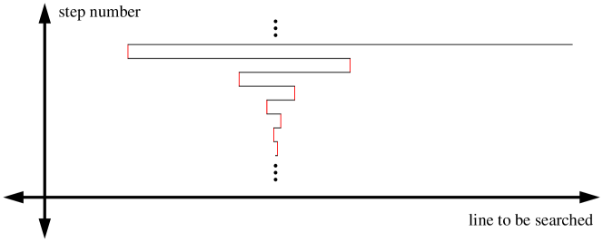
Figure 1: An optimal search trajectory for the linear-search problem: A geometric sequence without a first step.

In this paper, we study a clean and simple way to avoid the problems of geometric sequences without a first step, by assuming a constant turn cost $d$ for changing direction. This assumption is natural and realistic, as any reasonable scenario incurs some such cost for turning. We describe optimal trajectories for this scenario; as it turns out, they are generalizations of the optimal trajectories for the linear-search problem without turn cost, and have the same asymptotic behavior as $d\rightarrow 0$. The only previous work we are aware of that mentions turn cost in the context of the linear-search problem is [27], which considers (Section 2.5, p.25f.) a kinetic model, where turning takes a certain amount of time for braking and accelerating. It is shown that assuming a lower bound on OPT, a competitive ratio of 9 is still best possible for large OPT. (“Thus, as the braking time is of no relevance for large $n$, we know that the competitive ratio must be at least 9 as well.”) We go beyond this observation by cleanly quantifying the impact of turn cost on the overall search cost, and doing away with the assumption of a lower bound on OPT.

1.3 Other Related Work

Linear search problems occur in various contexts. See [1] for a study of rendezvous search on a line, where the objective of two players is to meet as fast as possible; this turns out to be a double linear-search problem. [24] studies randomized strategies for the star search (which is also known as the “cow-path problem”, motivated by a cow searching for the nearest pasture.) See [25] for more on the star search, and [20] for parallel searching.

Various types of search problems have been considered in a geometric (mostly two-dimensional) context. Here we only mention [9, 21, 28, 30], and the remarkable paper [22] that shows that online searching in a simple polygon can be performed with a competitive ratio of not more than 26.5. A very recent application in the context of robotics is described in [12, 13], where a robot has to stop every time it takes a scan of its environment; just like in this paper, the overall objective is to minimize total time until the discovery of an object hidden behind a corner, and this time is the sum of travel time and a cost for special points. However, the resulting trajectories and mathematical tools turns out to be quite different from what is presented here.

A good overview on search games can be found in the book [17], and the more recent book [2].

Relatively little work has been done on geometric optimization problems with turn cost. The interested reader may find some discussion in the paper [3].

1.4 Duality for Linear Programming

A standard tool for computing the values of two-player games is linear programming. In fact, studying such games was one of the origins of linear programming: An optimal strategy for one player can be interpreted as an optimal primal solution, while an optimal strategy for the second player corresponds to an optimal dual solution. (The reader unfamiliar with the basics of linear programming may turn to [10] for a good introduction.)

For finite games, the following results are well known (as weak duality and complementary slackness) and elementary to prove:

Proposition 1 (Weak duality, strong duality, complementary slackness)

Let $A$ be a finite real matrix and let $b,c$ be vectors of appropriate dimensions. Let $\max c^{t}x,Ax\leq b,x\geq 0$ be a primal linear program $(P)$, and let $\min b^{t}y,y^{t}A\geq c,y\geq 0$ be the corresponding dual linear program $(D)$.

Then weak duality holds: For any pair of feasible solutions, $x^{\prime}$ for $(P)$ and $y^{\prime}$ for $(D)$, we have $c^{t}x^{\prime}\leq b^{t}y^{\prime}$; if $c^{t}x^{\prime}=b^{t}y^{\prime}$ for any pair of feasible solutions, then $x^{\prime}$ is optimal for $(P)$ and $y^{\prime}$ is optimal for $(D)$.

Furthermore, strong duality holds: If $(P)$ is feasible and finitely solvable by $x^{*}$, then there exists a dual feasible solution $y^{*}$ with $c^{t}x^{*}=b^{t}y^{*}$.

For any such pair of optimal solutions, complementary slackness holds: If a dual variable $y_{j}$ is positive, then the corresponding primal constraint must hold with equality; if a primal constraint does not hold with equality, then the corresponding dual variable must be zero. Conversely, any pair of solutions satisfying complementary slackness is optimal.

The paper [23] also uses linear programs for the analysis of the cow-path problem; in particular, it uses these tools for analyzing the scenario where there is a known limit on the distance to the object. Considering turn cost makes our problem different; moreover, we use a different perspective of dealing with the issue of infinitely many constraints by considering dual variables for establishing a lower bound.

1.5 Our Results

Motivated by the linear-search problem with turn cost, we achieve a number of results.

$\bullet$ We establish duality results for certain types of infinite linear programs. As it turns out, this implies a verification method for the optimality of strategies.

$\bullet$ We show that the linear-search problem in the presence of turn cost can be characterized by an infinite linear program.

$\bullet$ Using CPLEX, we perform a computational study on the sequence of linear programs obtained by relaxing the infinite linear program to a linear subproblem with a finite number of constraints.

$\bullet$ From the computational results, we derive an analytic proof of the optimal strategies of searcher and hider. As a consequence of duality, the resulting bounds are tight: an optimal strategy requires $9$OPT$+2d$, and the optimal search strategy has step size $x_{i}=d\left(2^{i}-1\right)/2$.

$\bullet$ We also consider how the results vary if we allow the competitive ratio to increase at the benefit of decreasing the additive term.

$\bullet$ We generalize the above results to the scenario of star search by showing that the searcher can guarantee finding a solution within time

$$\left(1+2\frac{m^{m}}{(m-1)^{m-1}}\right)\mbox{OPT}+m\left(\left(\frac{m}{m-1}\right)^{m-1}-1\right)d$$

by choosing the strategy

$$x_{i}=d\left(\left(\frac{m}{m-1}\right)^{i+1}-1\right)/2.$$

$\bullet$ We show that for randomized strategies for searching on the line in the presence of turn cost, the same optimal competitive ratio $q=4.591121\ldots$ can be achieved as in the scenario without turn cost.

The rest of this paper is organized as follows. In Section 2, we describe basic results on infinite linear programs. In Subsection 3.1 we discuss the start of the search and show that the presence of turn cost always forces the existence of a first step with step length bounded from below. In Subsection 3.2 we derive an infinite linear program for the value of the game. Subsection 3.3 describes the results of a computational study; a clean analysis, with a mathematical proof of optimality of the derived strategies, is given in Section 3.4. Subsection 3.5 discusses the tradeoff between the coefficients of OPT and $d$. Section 4 describes the extension to star search. Section 5 gives a brief discussion on randomized strategies on the line. Some concluding thoughts are presented in Section 6.

2 Infinite Linear Programs

At first glance, linear programming and duality are not easily applicable to the search games described above, as the games are unbounded. However, we demonstrate that it makes sense to consider infinite linear programs. As it turns out, we can still construct primal and dual solutions, and prove optimality by applying weak duality. For this purpose, we construct infinite linear programs as the limit of increasingly large finite linear programs, obtained by successively adding variables and constraints. In the limit, a solution is an infinite sequence, instead of a finite vector; the scalar product of two vectors turns into the series of component products. When studying convergence, it helps to think of each solution vector of a finite linear program as a sequence that has zeroes for all unused variables.

Definition 2 (Infinite linear programs)

Let $c=(c_{i})_{i\in{\mathbbm{N}}}$ and $b=(b_{j})_{j\in{\mathbbm{N}}}$ be sequences of real numbers, and let $A=(a_{ij})_{i,j\in{\mathbbm{N}}}$ be a doubly indexed sequence of real numbers. Analogously, let $x=(x_{i})_{i\in{\mathbbm{N}}}$ and $y=(y_{j})_{j\in{\mathbbm{N}}}$ be sequences of real variables. Denote by $c^{(k)},b^{(k)},x^{(k)},y^{(k)}$ the vectors $(c_{1}\ldots,c_{k})$, $(b_{1}\ldots,c_{k})$, $(x_{1}\ldots,x_{k})$, and $(y_{1}\ldots,y_{k})$, respectively, and by $A^{(k)}$ the matrix $(a_{ij})_{i,j\in\{1,\ldots,k\}}$. Furthermore, we use the symbolic notation $c^{t}x:=\sum_{i=1}^{\infty}c_{i}x_{i}$ for the scalar product of two sequences. Let $(P^{(k)})$ be the $k$th subprogram, given by $\max{c^{(k)}}^{t}x^{(k)},A^{(k)}x^{(k)}\leq b^{(k)},x^{(k)}\geq 0$, and denote by $(D^{(k)})$ the corresponding $k$th dual linear program, given by $\min{b^{(k)}}^{t}y^{(k)},{y^{(k)}}^{t}A^{(k)}\geq c^{(k)},y^{(k)}\geq 0$. We say a sequence $x=(x_{i})_{i\in{\mathbbm{N}}}$ of nonnegative real numbers is a feasible solution for the infinite linear program given by $A,b,c$, if, for all $j\in{\mathbbm{N}}$, the constraint $\sum_{i=1}^{\infty}a_{ij}x_{i}\leq b_{j}$ holds; i.e., for all $k\in{\mathbbm{N}}$, $x^{(k)}$ is feasible for $(P_{k})$. An infinite linear program $(P)$, denoted by $\max c^{t}x,Ax\leq b,x\geq 0$, is the problem of finding a feasible solution that maximizes $c^{t}x$. A sequence $y=(y_{j})_{j\in{\mathbbm{N}}}$ of nonnegative real numbers is an infinite dual solution, if for all $i$, $c_{i}\leq\sum_{j=1}^{\infty}A_{ij}y_{j}<\infty$.

The following provides a way of establishing bounds for and optimality of feasible solutions for infinite linear programs.

Theorem 3 (Weak duality for infinite LPs)

Let $\max{c}^{t}x,Ax\leq b,x\geq 0$ be a an infinite linear program. Assume that the set $I:=\{i\in{\mathbbm{N}}\mid c_{i}\neq 0\}$ is finite, and that for any $i\in{\mathbbm{N}}$, all but finitely many $a_{ij}$ have the same sign. Let $x$ be a feasible solution for $(P)$, and let $y$ be an infinite dual solution. Then weak duality applies: ${c}^{t}x\leq{b}^{t}y$. Moreover, if ${c}^{t}x={b}^{t}y$, then $x$ is optimal.

Proof.

By the above assumptions, we have

$$c^{t}x=\sum_{i=1}^{\infty}c_{i}x_{i}=\sum_{i\in I}c_{i}x_{i}.$$

By assumption on $y$ it follows from $x_{i}\geq 0$ that

$$c^{t}x\leq\sum_{i\in I}x_{i}\sum_{j=1}^{\infty}a_{ij}y_{j}=\sum_{i\in I}\sum_{j=1}^{\infty}x_{i}a_{ij}y_{j}\leq\sum_{i=1}^{\infty}\sum_{j=1}^{\infty}x_{i}a_{ij}y_{j}.$$

For any $i$, only finitely many of the $a_{ij}$ have a sign different from the others, so the converging series $\sum_{j=1}^{\infty}x_{i}a_{ij}y_{j}$ is absolutely convergent. Furthermore, only finitely many $c_{i}$ can be negative, implying that all all but finitely many $\sum_{j=1}^{\infty}a_{ij}y_{j}$ are nonnegative. Thus, we may swap summations, getting

$$c^{t}x\leq y^{t}(Ax)=\sum_{j=1}^{\infty}\sum_{i=1}^{\infty}x_{i}a_{ij}y_{j}=\sum_{i=1}^{\infty}\sum_{j=1}^{\infty}x_{i}a_{ij}y_{j}=(y^{t}A)x\leq\sum_{j=1}^{\infty}b_{j}y_{j}=b^{t}y,$$

as claimed. ∎

The following motivates our approach to solving infinite linear programs by considering the sequence of finite subproblems. Assuming convergence of the sequences of primal and dual solutions, we get strong duality:

Theorem 4 (Strong duality for infinite LPs)

Let $\max{c}^{t}x,Ax\leq b,x\geq 0$ be a an infinite linear program. Assume that the set $I_{+}:=\{i\in{\mathbbm{N}}\mid c_{i}>0$ is finite. Let for all $k\in\mathbbm{N}$, $(P^{(k)})$ be feasible and bounded, and the sequence of primal optimal solutions be bounded; let $x^{*(k)}$ be a sequence of corresponding primal optimal solutions. For the corresponding sequence $\min{b}^{t}y^{(k)},{y^{(k)}}^{t}A^{(k)}\geq c,y^{(k)}\geq 0$ of dual linear programs $(D_{k})$, let $y^{*(k)}$ be a sequence of dual optimal solutions. Suppose that as $k$ tends to infinity, $x^{*(k)}$ converges componentwise to $x^{*}$ and $y^{*(k)}$ converges componentwise to $y^{*}$. Then $x^{*}$ is an optimal solution for the infinite linear program $(P)$. Moreover, strong duality holds, i.e., ${c^{*}}^{t}x^{*}={b^{*}}^{t}y^{*}$.

Proof.

We start by establishing primal feasibility of $x^{*}$: Suppose that inequality $(j)$ was violated by $x^{*}$, i.e., $\sum_{i=1}^{\infty}a_{ij}x_{i}>b_{j}$. As $a_{i\ell}=0$ for $\ell>j$, the first $j$ components of $x^{*}$ involved in $(j)$ form a point that has a positive distance from the set $\{z\in{\mathbbm{R}}^{j}\mid\sum_{i=1}^{j}a_{ij}z_{i}\leq b_{j}\}$. As for all $k\geq j$, inequality $(j)$ is part of $(P^{(k)})$, it must be satisfied by $x^{*(k)}$. This contradicts the fact that $x^{*(k)}$ converges towards $x^{*}$.

For $k>\max\{i\in I_{+}\}$, the sequence of objective values ${c^{(k)}}^{t}x^{*(k)}$ is monotonically decreasing, as for $k\leq\ell$, the feasible set for $(P^{(\ell)})$ is a subset of the feasible set for $(P^{(k)})$. As the sequence of objective values is bounded, $\lim_{k\rightarrow\infty}{c^{(k)}}^{t}x^{*(k)}$ exists. For any $k$, we have ${c^{(k)}}^{t}x^{*(k)}={b^{(k)}}^{t}y^{(k)}$ by strong duality. Thus, we have

$$c^{t}x^{*}=\lim_{k\rightarrow\infty}{c^{(k)}}^{t}x^{*(k)}=\lim_{k\rightarrow\infty}{b^{(k)}}^{t}y^{*(k)}=b^{t}y^{*}.$$

By Theorem 3, this implies optimality of $x^{*}$. ∎

Finally, complementary slackness holds; this will turn out to be a useful tool for determining dual variables, and thus for proving optimality.

Theorem 5 (Complementary slackness for infinite LPs)

Let $\max{c}^{t}x,Ax\leq b,x\geq 0$ be a an infinite linear program. Assume that the set $I:=\{i\in{\mathbbm{N}}\mid c_{i}\neq 0\}$ is finite, and that for any $i\in{\mathbbm{N}}$, all but finitely many $a_{ij}$ have the same sign. Let $x$ be a feasible solution for $(P)$, and $y$ be an infinite dual solution. Then $x$ and $y$ are optimal if and only if the following complementary slackness conditions hold:

(a) For any $i\in{\mathbbm{N}}$ with $\sum_{j=1}^{\infty}y_{j}a_{ij}>c_{i}$, $x_{i}=0$ holds.

(b) For any $i\in{\mathbbm{N}}$ with $x_{i}>0$, $\sum_{j=1}^{\infty}y_{j}a_{ij}=c_{i}$ holds.

(c) For any $j\in{\mathbbm{N}}$ with $\sum_{i=1}^{\infty}a_{ij}x_{i}<b_{i}$, $y_{j}=0$ holds.

(d) For any $j\in{\mathbbm{N}}$ with $y_{j}>0$, $\sum_{i=1}^{\infty}a_{ij}x_{i}=b_{i}$ holds.

Proof.

By assumptions, all involved series are absolutely convergent. Thus we get $(y^{t}A)x\geq c^{t}x\Leftrightarrow(y^{t}A-c)x\geq 0$, and $y^{t}b\geq y^{t}(Ax)\Leftrightarrow y^{t}(b-Ax)\geq 0$. Now it is easy to check that $y^{t}b=c^{t}x$, iff the stated conditions hold. ∎

We believe that the above tools are useful and applicable in various game-theoretic scenarios, even when there is no clear idea of a possible optimal strategy. We demonstrate the practical applicability by giving the results of a computational study performed with CPLEX [11], a commercially available software package for solving linear programs, and showing how these results enable us to give a tight (theoretical) analysis of the cost of an optimal search strategy in the presence of turn cost. It should be noted that in this paper, the numerical experiments are only a stepping stone towards finding optimal strategies: The idea is to identify closed-form limiting solutions; once those are found and verified by using duality, numerical accuracy is not an issue. That means that the numerical results could be omitted without impeding the proof of optimality of the resulting strategies. However, our approach should also prove useful for other problems, even if no optimal closed-form strategy can be deduced from solving finite subsystems: In those cases, we can still give bounds on the possible performance of strategies. Only in those cases, issues of numerical stability come into play.

3 Searching on the Line with Turn Cost

3.1 The First Move and an Additive Term

In the presence of a positive turn cost $d$, the hider can make it impossible for the searcher to achieve a competitive ratio, by simply placing the object arbitrarily close to the origin, on the side that is not picked first by the searcher. Clearly, this requires a minimum cost of $d$, regardless of OPT. Moreover, the searcher will be forced to make a second turn if she starts with a too small (or infinitesimal) first step. This increases the minimum cost.

We show that the optimal competitive ratio, $c$, remains the same even if we add turn cost. Thus, the worst-case time to reach the target is $c\cdot$OPT plus some additive term, denoted $B$, that we wish to minimize. Determining the minimum value of $B$ is one of the main objectives of this paper.

It is clear that even in the presence of a fixed additive term, the searcher will not be able to achieve any competitive ratio at all if she uses a large number of steps before first reaching a distance of $d$ from the origin. In particular, it can easily be seen that she is forced to make a first step of length $x_{1}=\Omega(d)$. We will use this observation in the following subsections for a more careful analysis.

3.2 An Infinite Linear Program

Suppose that the searcher carries out a sequence of step lengths $x_{1},x_{2},\ldots$ from the origin, where $x_{1},x_{3},\ldots$ are increasing distances to the right, while $x_{2},x_{4},\ldots$ are increasing distances to the left. In the following, we denote these turn positions by $p_{i}=(-1)^{i+1}x_{i}$.

For a given sequence of step lengths $x_{i}$, the hider can choose the possible set of locations $y_{i}=(-1)^{i+1}(x_{i}+\varepsilon)$ for an arbitrarily small $\varepsilon$. If the object is placed at $y_{n}$, the searcher will only encounter it after traveling a distance of $(\sum_{i=1}^{n+1}2x_{i})+x_{n}+\varepsilon$, and making $n+1$ turns. Note that for arbitrarily small $d$, this approaches the linear-search problem, with a competitive ratio of 9. In order to guarantee this competitive ratio, and an additive cost of $B$, the corresponding search trajectories satisfy

$$2x_{1}+\ldots+2x_{i-2}+3x_{i-1}+2x_{i}+id+\varepsilon\leq 9(x_{i-1}+\varepsilon)+B.$$

As all $x_{i}$ are bounded away from zero, and the above condition must hold for any $\varepsilon>0$, we conclude that

$$2x_{1}+2x_{2}+\ldots+2x_{i-2}+3x_{i-1}+2x_{i}+id\leq 9x_{i-1}+B.$$

or

$$2x_{1}+2x_{2}+\ldots+2x_{i-2}-6x_{i-1}+2x_{i}+id\leq B.$$

We thus get the following infinite linear program:

$$\begin{array}[]{rcrcrcrcrcrcrcr}&&\min&B\\ 2x_{1}&&&&&&&&&&&+&d&\leq&B\\ -6x_{1}&+&2x_{2}&&&&&&&&&+&2d&\leq&B\\ 2x_{1}&-&6x_{2}&+&2x_{3}&&&&&&&+&3d&\leq&B\\ 2x_{1}&+&2x_{2}&-&6x_{3}&+&2x_{4}&&&&&+&4d&\leq&B\\ \vdots&+&\vdots&-&\vdots&+&\vdots&&&&&+&\vdots&\leq&B\\ 2x_{1}&+&2x_{2}&+&\cdots&+&2x_{i-2}&-&6x_{i-1}&+&2x_{i}&+&id&\leq&B\\ \vdots&&\vdots&&\vdots&&\vdots&&\vdots&&\vdots&&\vdots&\leq&B\\ &&&&&&&&&&x_{i}&&&\geq&0.\\ \end{array}$$ (1)

3.3 Solving the Sequence of Linear Programs

Even with sophisticated software, it is impossible to solve an infinite linear program to optimality. However, for each $n$, the first $n$ linear inequalities describe a relaxation of the overall program. Denote $\lambda=B/d$, and let $\lambda_{n}$ be the optimal value when only considering the first $n$ constraints. Then any $\lambda_{n}$ is a lower bound on the overall $\lambda$. Furthermore, the sequence of primal optimal values $x_{i}^{(n)}$ and dual optimal values $y_{i}^{(n)}$ should converge, if there is any hope for an overall solution.

We have solved a number of these relaxations by using CPLEX 7.1. The computational results are shown in Table 1. Shown are the number of constraints that we used, the optimal value $\lambda_{n}$, the first five primal variables, and the first five dual variables. To allow numerical computation, $d$ was normalized to 1. As each $\lambda_{n}$ is a valid lower bound, numbers were truncated, not rounded.

$n$	$\lambda_{n}$	$x_{1}^{(n)}$	$x_{2}^{(n)}$	$x_{3}^{(n)}$	$x_{4}^{(n)}$	$x_{5}^{(n)}$	$y_{1}^{(n)}$	$y_{2}^{(n)}$	$y_{3}^{(n)}$	$y_{4}^{(n)}$	$y_{5}^{(n)}$
1	1.0000	0.0000
2	1.2500	0.1250	0.0000				0.7500	0.2500
3	1.4166	0.2083	0.3333	0.0000			0.6666	0.2500	0.0833
4	1.5312	0.2656	0.5625	0.6875	0.0000		0.0625	0.2500	0.0937	0.0312
5	1.6125	0.3062	0.7250	1.1750	1.3000	0.0000	0.6000	0.2500	0.1000	0.0375	0.0125
6	1.6718	0.3359	0.8437	1.5312	2.2500	2.3750	0.5833	0.2500	0.1041	0.0416	0.0156
7	1.7165	0.3582	0.9330	1.7991	2.9642	4.1607	0.5714	0.2500	0.1071	0.0446	0.0178
8	1.7509	0.3754	1.0019	2.0058	3.5156	5.5930	0.5625	0.2500	0.1093	0.0468	0.0195
9	1.7782	0.3891	1.0563	2.1692	3.9130	6.6284	0.5555	0.2500	0.1111	0.0486	0.0208
10	1.8001	0.4000	1.1003	2.3011	4.3031	7.5078	0.5500	0.2500	0.1125	0.0500	0.0218
20	1.9000	0.4500	1.3000	2.9000	5.9000	11.5000	0.5250	0.2500	0.1187	0.0562	0.0265
30	1.9333	0.4666	1.3666	3.1000	6.4333	12.8333	0.5166	0.2500	0.1208	0.0583	0.0281
40	1.9500	0.4750	1.4000	3.2000	6.7000	13.5000	0.5125	0.2500	0.1218	0.0593	0.0289
50	1.9600	0.4800	1.4200	3.2600	6.8600	13.9000	0.5100	0.2500	0.1225	0.0600	0.0293
100	1.9800	0.4900	1.4600	3.3800	7.1800	14.7000	0.5050	0.2500	0.1237	0.0612	0.0303
200	1.9900	0.4950	1.4800	3.4400	7.3400	15.1000	0.5025	0.2500	0.1243	0.0618	0.0307
400	1.9950	0.4975	1.4900	3.4700	7.4200	15.3000	0.5012	0.2500	0.1245	0.0621	0.0310

Table 1: Solutions for a number of linear subsystems.

The table illustrates several points:

1. Even small subsystems may have “ugly” solutions, indicating a relatively fast increasing effort for trying to establish lower bounds by analyzing subsystems manually.

2. Convergence is rather slow; in fact, it seems to be logarithmic, as doubling the size of the system appears to cut the remaining error in half. This and the tediousness of the solutions make it rather difficult to give an explicit closed formula for the objective values, which could be used for analyzing the limit. This justifies the use of powerful tools like CPLEX in order to get good estimates quickly.

3. Actually closing the remaining gap in order to prove that the lower bound of 9OPT$+2d$ is tight requires considering the whole infinite linear program.

We will demonstrate in the following subsection how the latter point can be carried out analytically.

3.4 Provably Optimal Strategies

To establish optimal strategies for the infinite linear program, and thus a pair of optimal strategies, we start by describing a feasible dual solution that yields a lower bound of 2 for the objective value $\lambda$.

Consider $y_{j}=\frac{1}{2^{j}}$. We will show that with these dual multipliers, the linear combination of the first $n$ coefficients for any variable $x_{j}$ tends to $0$, as $n$ approaches infinity. More precisely, taking a linear combination of all inequalities in (1), with coefficient $y_{j}$ used for inequality $j$, yields

$$2\left(\sum_{j=1}^{\infty}y_{j}-8y_{2}\right)x_{1}+2\left(\sum_{j=2}^{\infty}y_{j}-8y_{3}\right)x_{2}+\cdots+2\left(\sum_{j=i}^{\infty}y_{i}-8y_{i+2}\right)x_{i}+\cdots+\left(\sum_{j=1}^{\infty}jy_{j}\right)d$$

$$\leq \left(\sum_{j=1}^{\infty}y_{j}\right)B$$

Using $y_{j}=\frac{1}{2^{j}}$, the involved series and coefficients do converge: The coefficient of $x_{i}$ becomes

$$-\frac{8}{2^{i+1}}+\sum_{j=i}^{\infty}\frac{2}{2^{j}}=\frac{1}{2^{i}}\left(-4+2\sum_{i=0}^{\infty}\frac{1}{2^{j}}\right).$$

Thus, this turns out to be $0$.

Similarly, the coefficient of $d$ becomes $\sum_{i=j}^{n}\frac{j}{2^{j}}$, which tends to $2$ as $n$ grows.

Finally, the coefficient of $B$ on the right hand side of the inequality is the geometric series $\sum_{i=1}^{n}\frac{1}{2^{j}}$, which tends to $1$.

Therefore, the derived inequality simplifies to the lower bound

$$2d\leq B.$$

To see that $2d$ is also an upper bound, and thus an optimal solution for $B$, consider $x_{i}=(2^{i}-\frac{1}{2})d$. For this particular set, the $j$th inequality becomes

$$\left(\sum_{h=1}^{i}2x_{h}\right)-8x_{j-1}+jd\leq B,$$

which simplifies to

$$2d\leq B.$$

Thus, the linear program becomes

$$\begin{array}[]{rcc}&\min&\lambda\\ 2&\leq&\lambda.\end{array}$$ (2)

Trivially, this is solved by $\lambda=2$, implying that the given $x_{i}$ and $\lambda=2$ do indeed provide a feasible solution with objective value 2. By duality of linear programming, this is optimal.

It should be noted that the primal and dual solutions satisfy complementary slackness, as all constraints hold with equality. Note that our solution to the linear-search problem with turn cost achieves a competitive ratio of 9, which must be the optimal value because the time to find the target increases with $d>0$.

We summarize:

Theorem 6

In the presence of turn cost $d$ for the linear-search problem, the searcher can guarantee a solution within time 9OPT$+2d$ by choosing the search strategy $x_{i}=d(2^{i}-1)/2$. The additive term $2d$ is minimal subject to the optimal competitive ratio, 9.

Note that the overall total cost spent on turning is about $\log_{2}$ OPT.

3.5 Tradeoff between Coefficients

The term $2d$ is best possible if we want to maintain the best possible competitive factor of $9$. It may be desirable to improve the former term, while allowing an increase in the latter. For any bound $c\geq 9$ on the competitive ratio, the best possible $B$ can be computed by using our above approach: In the system (1), replace all coefficients $-6$ by $3-c$. Conversely, we can compute the best possible $c$ for any $B/d\in(1,2]$. The resulting tradeoff curve is shown in Figure 2. This curve was obtained experimentally using CPLEX. We have not yet characterized it analytically, though we expect that to be possible. It is not hard to see that $1$ is a lower bound for any $B/d$, and that the best possible $B/d$ tends to $1$ for $c$ approaching infinity.

Figure 2: Tradeoff between competitive factor and turn cost.

4 Star Search

For the problem with no turn cost, Gal [17] proved that the sequence of turning points corresponding to an optimal search trajectory has to be cyclic. In the following, we show how to generalize the above results to the problem of star search in the presence of turn cost.

As before, we consider a sequence $x_{1},x_{2},\ldots$ of steps that cycle through the $m$ rays. Suppose we have a turn cost of $d_{1}$ on a ray, and $d_{2}$ at the origin; set $d=d_{1}+d_{2}$. By picking a hiding spot just beyond one of the turning points, the hider can force the searcher to find the object only after making moves $x_{n},\ldots,x_{n+m-1}$ and returning to the ray of $x_{n}$, making a total of $(n+m-1)$ turns. This takes a time of $\left(2\sum_{i=1}^{n+m-1}x_{i}\right)+(n+m-1)d+x_{n}$ instead of the optimal $x_{n}$. Without the presence of turn cost, it is well known that the optimal competitive ratio is $\left(1+2\frac{m^{m}}{(m-1)^{m-1}}\right)=:1+2M$. When the hiding point is close to the start, the searcher may only get to it when entering the last ray, so we get the condition

$$\left(2\sum_{i=1}^{m-1}x_{i}\right)+(m-1)d\leq B.\hfill(m-1)$$

If the hiding point is just beyond the $n$th turning point, we get the condition

$$\left(2\sum_{i=1}^{n+m-1}x_{i}\right)+(n+m-1)d+x_{n}\leq B+(1+2M)x_{n},$$

or

$$\left(2\sum_{i=1}^{n+m-1}x_{i}\right)+(n+m-1)d\leq B+2Mx_{n}.\hfill(n)$$

for the additive term $\lambda$, if it exists. For convenience, we refer to the dual variables corresponding to constraints $(m-1),\ldots,(n),\ldots$ as $y_{m-1},\ldots,y_{n},\ldots$.

Again, finding a strategy $x_{1},x_{2},\ldots$ that minimizes $B$ subject to the above constraints can be described as an infinite linear program. For $m=3,4,5,6$ and various $n$ up to 1000, we solved the finite subprograms by using CPLEX. Despite some numerical difficulties, we were able to extrapolate the limits of the series by making use of the logarithmic convergence. We obtained the following solutions:

$$x_{i}=d\left(\left(\frac{m}{m-1}\right)^{i}-1\right)/2$$

and

$$B=m\left(\left(\frac{m}{m-1}\right)^{m-1}-1\right)d=(M-m)d.$$

Note that finding $x_{i}$ is also possible without deriving a closed-form solution directly from CPLEX experiments: If $y_{j}>0$ for all $j\in{\mathbbm{N}}$, complementary slackness (Theorem 5) requires that all constraints hold with equality. Then subtracting constraint $(n+m-1)$ from constraint $(n+m)$ yields the recursion $2x_{m-1+n}+d=2Mx_{n}$, which is satisfied by the above solution.

Theorem 7

In the presence of turn cost $d$ for the star search problem on $m$ rays, the searcher can guarantee a solution within time

$$\left(1+2\frac{m^{m}}{(m-1)^{m-1}}\right){\rm OPT}+m\left(\left(\frac{m}{m-1}\right)^{m-1}-1\right)d$$

by choosing the search strategy

$$x_{i}=d/2\left(\left(\frac{m}{m-1}\right)^{i+1}-1\right).$$

This strategy is optimal.

Proof.

We show that this primal strategy and $B$ satisfy all constraints of the linear program with equality: The left-hand side of inequality $(n)$ is

$$2\left(\sum_{i=1}^{n+m-1}x_{i}\right)+(n+m-1)d.$$

Using $q:=\frac{m}{m-1}$ and substituting the values $x_{i}=d(q^{i}-1)/2$, this simplifies to

$$\frac{q^{n+m}-q}{q-1}d.$$

On the other hand, by substituting the above values, the right-hand side

$$B+\left(2\frac{m^{m}}{(m-1)^{m-1}}\right)x_{n}$$

becomes

$$m\left(q^{m-1}-1\right)d+mq^{m-1}\left(q^{n}-1\right)d$$

or (using $m=\frac{q}{q-1}$)

$$\frac{q^{n+m}-q}{q-1}d.$$

Therefore, with $B=m\left(\left(\frac{m}{m-1}\right)^{m-1}-1\right)d$, all constraints are satisfied with equality, regardless of $n$.

It remains to be shown that the above solution is best possible. In principle, this can be done by figuring out explicit closed-form expressions for the dual variables, and using them to verify optimality. (The interested reader may try this for $m=3$, where the dual variables turn out to be $y_{j}=\frac{4(2^{j-1}+(-1)^{j})}{3^{j+1}}$ for $j\geq m-1=2$, i.e., the sequence 4/9, 4/27, 4/27, 20/243, 44/729,…) However, this explicit approach appears to be extremely tedious for any $m>3$, and hopeless for general $m$. As we will see in the following, finding an explicit closed-form expression for dual variables is not necessary for a proof of optimality. Instead, we use complementary slackness to derive a recursive characterization of $y$, and verify that it satisfies all required conditions.

As any solution $x_{1},\ldots$ describing a valid strategy must satisfy $x_{i}>0$ for all $i\geq 1$, we conclude by Theorem 5 that all corresponding dual constraints must hold with equality; as $c_{i}=0$ for all $x_{i}$, this means that

$$\left(2\sum_{j=i}^{\infty}y_{j}\right)=2My_{i+m-1}\hfill(i)$$

must hold for all $i\in{\mathbbm{N}}$, with $y_{1}=\ldots=y_{m-2}=0$ for ease of notation. Noting that we are trying for a nonnegative $y$ (and thus an absolutely convergent series $\sum_{j=i}^{\infty}y_{j}$), subtracting this condition $(i)$ for $i=n\geq m-1$ from the condition for $i=n+1$ yields

$$y_{n+1}=M(y_{n+m}-y_{n+m-1}),$$

i.e., the recursion

$$y_{n+m}=y_{n+m-1}-\frac{1}{M}y_{n}.$$

Because the cost coefficient $c_{B}$ of $B$ is $-1$, we get the requirement $\sum_{j=m-1}^{\infty}y_{j}=1$, which implies $y_{m}=\ldots=y_{2m-2}=1/M$ by conditions $(1),\ldots,(m-1)$. Choosing $y_{m-1}=m/M$, we get a well-defined sequence $y$. Using the initial condition $y_{2m-2}=1/M$, the recursive condition implies $y_{n+m}=\frac{1}{M}(1-\sum_{j=m-1}^{n}y_{j})$. Because of $\frac{m}{M}=\frac{(m-1)^{m-1}}{m^{m-1}}=\left(1-\frac{1}{m}\right)^{m}\in[1/3,1/2]$, the series $\sum_{j=m-1}^{\infty}y_{j}=\lim_{n\rightarrow\infty}\sum_{j=m-1}^{n}y_{j}$ does indeed tend to 1. (In fact, not only does $y_{j+m}/y_{j}$ tend to $m/M$ for large $j$, but the ratio $y_{j}/y_{j-1}$ tends to $\left(\frac{m-1}{m}\right)$.) For the given starting values, the sequence $\sum_{j=m-1}^{n}y_{j}$ remains below 1, so the sequence $y_{n+m}$ remains nonnegative.

It remains to be shown that $y^{t}b=c^{t}x$, i.e., $\sum_{j=m-1}^{\infty}jy_{j}=M-m$. This follows from

$$\sum_{j=m-1}^{\infty}jy_{j} = \sum_{j=m-1}^{2m-2}jy_{j}+\sum_{j=2m-1}^{\infty}jy_{j}$$

$$= \sum_{j=m-1}^{2m-2}jy_{j}+\sum_{j=m-1}^{\infty}(j+m)y_{j+m}$$

$$= \sum_{j=m-1}^{2m-2}jy_{j}+\sum_{j=m-1}^{\infty}(j+m)(y_{j+m-1}-\frac{1}{M}y_{j})$$

$$= (2m-2)y_{2m-2}+\sum_{j=m-1}^{2m-3}jy_{j}+\sum_{j=m-1}^{\infty}(j+m-1)y_{j+m-1}+\sum_{j=m-1}^{\infty}y_{j+m-1}$$

$$-\sum_{j=m-1}^{\infty}\frac{1}{M}jy_{j}-\sum_{j=m-1}^{\infty}\frac{m}{M}y_{j}$$

$$= \frac{2m-2}{M}+\sum_{j=m-1}^{\infty}jy_{j}+\left(1-\sum_{j=m-1}^{2m-3}y_{j}\right)-\sum_{j=m-1}^{\infty}\frac{1}{M}jy_{j}-\frac{m}{M},$$

hence

$$\sum_{j=m-1}^{\infty}jy_{j}=2m-2+(M-m-(m-2))-m=M-m,$$

as claimed. ∎

5 Randomized Strategies

Consider the search on the line with turn cost. It is natural to consider randomized strategies for both players: The particular choice of search strategy or hiding position depends on the outcome of a random event that is not known in advance. It is known that the optimal competitive ratio $q=1+a$ for online searching on the line without turn cost is given by the solution of the equation satisfying $\frac{a+1}{\ln a}=a$, or $q=4.591121\ldots$; see [2], pp. 129/130. Clearly, the optimal coefficient $q_{t}$ of OPT in the presence of turn cost must satisfy $q_{t}\geq q$. To see that there is indeed a strategy that achieves $q_{t}=q$, consider a modified scenario without turn cost as follows:

1. The searcher only locates the hider after passing the hider by a length of at least $d/2$.

2. When discovering the hider, the cost is the distance traveled, minus $d/2$.

Then the resulting calculations from [2] translate precisely to the scenario with turn cost. Using the same turning points $x_{i}\geq d/2$, we get a mixed strategy that assures a cost of $q(OPT+d/2)-d/2=qOPT+d(q-1)/2$. The additive constant can be improved, as the terms below $d/2$ are not used. We conclude:

Theorem 8

For randomized strategies in the presence of turn cost, the optimal coefficient of OPT is the same as without turn cost.

Again it is possible to consider the optimal coefficient of the turn-cost factor, and also consider the tradeoff between both coefficients. We leave this to future research.

6 Conclusions

In this paper we have considered the linear-search problem in the presence of turn cost. We have shown that this extends the well-studied case without turn cost, and established a performance guarantee of 9OPT$+2d$. We also extended or results to the general star search on $m$ rays (also known as the cow-path problem), and showed that this problem can also be resolved by using an infinite sequence of linear programs.

We believe that our methods and results can be easily extended to various other problems that have been studied; in particular, it should not be too hard to give explicit estimates for the lower-order terms, which show up if the distance OPT to the hidden object is known to be bounded by some $D$: This only requires giving an explicit estimate for the solutions of subsystems of size $n=\Theta(\log D)$.

Just like the cow-path problem extends to various geometric scenarios, we expect that there are also many other problems for which the cost of changing the search direction plays an important role.

References

- [1] S. Alpern and A. Beck. Pure strategy asymmetric rendezvous on the line with an unknown initial distance. Operations Research, 48 (2000), 498–501.
- [2] S. Alpern and S. Gal. The Theory of Search Games and Rendezvous. Kluwer Academic Publishers.
- [3] E. Arkin, M. Bender, E. Demaine, S. P. Fekete, J. S. B. Mitchell, S. Sethia. Optimal covering tours with turn costs. Proceedings SODA 01, ACM-SIAM Symposium on Discrete Algorithms, 2001, 138–147.
- [4] R. A. Baeza-Yates, J. C. Culberson, and G. J. E. Rawlins. Searching with uncertainty. Proceedings SWAT 88, First Scandinavian Workshop on Algorithm Theory. Springer Lecture Notes in Computer Science #318, 1988, 176–189.
- [5] R. A. Baeza-Yates, J. C. Culberson, and G. J. E. Rawlins. Searching in the plane. Information and Computation, 106 (1993), 234–252.
- [6] A. Beck. On the linear search problem. Naval Research Logistics, 2 (1964), 221–228.
- [7] A. Beck and D. J. Newman. Yet more on the linear search problem. Israel Journal of Mathematics, 8 (1970), 419–429.
- [8] R. Bellman. An optimal search problem. SIAM Reviews, 5 (1963), 274.
- [9] C. A. Brocker and S. Schuierer. Searching rectilinear streets completely. Proceedings WADS 99, Workshop on Algorithms and Data Structures, Springer Lecture Notes in Computer Science, # 1663, 1999, 98–109.
- [10] V. Chvátal. Linear Programming. Freeman, New York, 1983.
- [11] CPLEX. http://www.ilog/com/products/cplex.
- [12] S. P. Fekete, R. Klein, and A. Nüchter. Online searching with an autonomous robot, 2004. Proceedings of the Workshop on Algorithmic Foundations of Robotics, to appear in Algorithmic Foundations of Robotics VI, Springer-Verlag.
- [13] S. P. Fekete, R. Klein, A. Nüchter. Searching with an autonomous robot. (Video + abstract). In 20th ACM Symposium on Computational Geometry, 2004, 449–450.
- [14] A. Fiat and G. J. Woeginger. Online optimization, the state of the art. Springer Lecture Notes in Computer Science, # 1442, 1998.
- [15] S. Gal. A general search game. Israel Journal of Mathematics, 12 (1972), 32–45.
- [16] S. Gal. Minimax solutions for linear search problems. SIAM Journal on Applied Mathematics, 27 (1974), 17–30.
- [17] S. Gal. Search Games. Academic Press, New York, 1980.
- [18] S. Gal and D. Chazan. On the optimality of the exponential functions for some minimax problems. SIAM Journal on Applied Mathematics, 30 (1976), 324–348.
- [19] M. Grötschel, S. Krumke, and J. Rambau. Online optimization of large scale systems: the state of the art. Springer-Verlag 2001.
- [20] M. Hammar, B. J. Nilsson, and S. Schuierer. Parallel searching on rays. Proceedings STACS 99, Symposium on Theoretical Aspects of Computer Science, Springer Lecture Notes in Computer Science, # 1563, 1999, 132–142.
- [21] C. Hipke, C. Icking, R. Klein, and E. Langetepe. How to find a point on a line within a fixed distance. Discrete Applied Mathematics, 93 (1999), 67–73.
- [22] F. Hoffmann, C. Icking, R. Klein, and K. Kriegel. The polygon exploration problem. SIAM Journal on Computing, 31 (1999), 577–600.
- [23] P. Jaillet and M. Stafford. Online searching. Operations Research 49 (2001), 501–515.
- [24] M. Y. Kao, J. H. Reif, and S. R. Tate. Searching in an unknown environment: an optimal randomized algorithm for the cow-path problem. Information and Computation, 131 (1996), 63–79.
- [25] O. Kella. Star search—a different show. Israel Journal of Mathematics, 81 (1993), 145–159.
- [26] D. E. Knuth. Searching and Sorting. Addison Wesley, 1973.
- [27] A. Lopez-Ortiz. Searching in bounded and unbounded domains. PhD Thesis, Department of Computer Science, University of Waterloo, 1996. Also available as technical report CS-96-25.
- [28] A. Lopez-Ortiz and S. Schuierer. Position-independent near optimal searching and on-line recognition in a star polygon. Proceedings WADS 97, Workshop on Algorithms and Data Structures, Springer Lecture Notes in Computer Science, # 1272, 1997, 284–296.
- [29] A. Lopez-Ortiz and S. Schuierer. The ultimate strategy to search on rays?, Theoretical Computer Science, 261 (2001), 267–295.
- [30] S. Schuierer. Lower bounds in on-line geometric searching. Computational Geometry—Theory & Applications, 18 (2001), 37–53.