Directional Consistency for
Continuous Numerical Constraints

Abstract

Bounds consistency is usually enforced on continuous constraints by first decomposing them into binary and ternary primitives. This decomposition has long been shown to drastically slow down the computation of solutions. To tackle this, Benhamou et al. have introduced an algorithm that avoids formally decomposing constraints. Its better efficiency compared to the former method has already been experimentally demonstrated. It is shown here that their algorithm implements a strategy to enforce on a continuous constraint a consistency akin to Directional Bounds Consistency as introduced by Dechter and Pearl for discrete problems. The algorithm is analyzed in this framework, and compared with algorithms that enforce bounds consistency. These theoretical results are eventually contrasted with new experimental results on standard benchmarks from the interval constraint community.

1 Introduction

Waltz’s seminal paper [15] promoted the idea of local consistency enforcement to solve constraints. Systems of constraints were solved by considering each of them in turn, discarding the values in the domains of the variables involved that could not possibly be part of a solution. Montanari [13] and Mackworth [11] introduced the notion of a network of constraints in which a more involved scheme for propagating domain modifications could be used. Davis [4] later adapted these works to solve continuous problems by employing interval arithmetic [14] to handle the domains of the variables.

The first solvers to implement the ideas of Davis and others were enforcing on continuous constraints a relaxation of arc consistency, bounds consistency (aka 2B consistency [10]), which is better suited to real domains. For practical reasons, bounds consistency can only be effectively enforced on binary and ternary constraints. More complex constraints then have to be decomposed into such simpler constraints, thereby augmenting the number of variables and constraints to eventually consider. Benhamou, van Hentenryck, and McAllester [2] produced experimental evidences that such a process drastically slows down the computation, rendering in effect bounds consistency computation impracticable on many problems. They then advocated to replace bounds consistency altogether by a new consistency notion, box consistency, whose enforcement does not require the decomposition of complex constraints.

However, in 1999, Benhamou et al. presented the HC4 algorithm [1], which is strongly related to the methods employed to enforce bounds consistency except for its ability to handle constraints without formal decomposition. HC4 was shown to outperform box consistency-based solvers on some large problems; in addition, its use in a suitable cooperation scheme was recommended to speed up the computation of box consistency on difficult problems. In their paper, the authors did not analyze HC4 on a theoretical point-of-view. They claimed, however, that it would enforce bounds consistency on the system of primitive constraints stemming from the decomposition of a constraint containing no more than one occurrence of any variable.

The contribution of this paper is to present an analysis of the HC4 algorithm and to compare it from the theoretical point-of-view with the HC3 algorithm used to enforce bounds consistency on decomposed constraints. We also characterize the consistency HC4 enforces on one constraint in terms of the equivalent on continuous domains of directional bounds consistency introduced by Dechter and Pearl [6], and we prove Benhamou et al.’s claim concerning it computing bounds consistency for constraints with variables occurring at most once. Lastly, we analyze experimental results to justify the discrepancy they exhibit with theoretical results.

To offer a reasonably self-content exposition, we start by recalling some definitions and algorithms related to the solving of discrete Constraint Satisfaction Problems (CSP) in Section 2; We then adapt in Section 3 the framework just introduced to the case of continuous CSPs, thus emphasizing the parallel between algorithms presented by Dechter [5] to enforce Directional Arc Consistency and the HC4 algorithm; The complexity of HC4 and HC3 are compared in Section 4, first for one constraint only in Section 4.1, and then on a constraint system in Section 4.2; in Section 5, we contrast the theoretical results obtained in the previous sections with experimental results obtained on a set of standard benchmarks; finally, we analyze our results in Section 6, and we propose some other interpretations of the HC4 algorithm that could lead to more efficient algorithms.

2 Local Consistency Techniques for Discrete Problems

The entities we will manipulate in the sequel of this paper are variables from an infinite countable set $\{x_{1},x_{2},\dots\}$, with their associated domains of possible values $D[x_{1}]$, $D[x_{2}]$, …, and constraints, which enforce some relation between variables. A constraint $C$ on a finite set of variables $S[C]$—its scope—with domains $D$ is a subset of the product of their domains.

A constraint problem $P$ is formally characterized by a triplet $(V,D,R)$, where $V$ is a finite set of variables with domains $D$, and $R$ is a set of constraints such that the union of their scopes is included in $V$.

The basic step to solve a constraint problem corresponds to the inspection of each of its constraints $C$ in turn and to the removal of all the values in the domains of the variables in $S[C]$ that cannot be part of a solution of $C$. To this end, we need to be able to project $C$ onto each of its variables. This notion of projection is formally stated below.

Definition 1 (Projection of a constraint)

Let $C$ be a constraint, $D$ a Cartesian product of domains, and $x$ a variable in $C$. The projection of $C$ on $x$ w.r.t. $D$ is the set $\Pi(C,D,x)$ of values in $D[x]$ that can be extended to a solution of $C$ in $D$.

A projection is then the set of consistent values of a variable relative to a constraint. The well-known arc consistency property [11] demands that all values in a domain be consistent. This property is clearly too strong for our purpose since it has no practical counterpart for continuous domains in the general case. We will then only consider a weaker consistency notion that restricts itself to the bounds of the domains: bounds consistency.

Definition 2 (Bounds consistency)

Given $C$ a constraint, $D$ a Cartesian product of domains, and $x$ a variable in $S[C]$, $x$ is said bounds consistent w.r.t. $C$ and $D[x]$ if and only if the following property holds:

$$\min(D[x])\in\Pi(C,D,x)\ \wedge\ \max(D[x])\in\Pi(C,D,x)$$

A constraint $C$ is said bounds consistent w.r.t. a Cartesian product of domains $D$ if and only if every variable $x$ in its scope is bounds consistent relative to $C$ and $D[x]$. A constraint system is bounds consistent w.r.t. $D$ if and only if each of its constraints is bounds consistent w.r.t. $D$.

Solving a constraint problem $P$ means computing all tuples of the product of domains that satisfy all the constraints. The general algorithm is a search strategy called backtracking. The computation state is a search tree whose nodes are labelled by a set of domains. The backtracking algorithm requires a time exponential in the number of variables in the worst case. Its performances can be improved with local consistency enforcement to reduce the domains prior to performing the search. For instance, the domain of a variable $x$ that is not bounds consistent relative to a constraint $C$ can be reduced by the following operation:

$$\mathrm{\mathop{ReviseBounds}}(C,D,x)=[\min(D[x]\cap\Pi(C,D,x)),\max(D[x]\cap\Pi(C,D,x))]$$ (1)

The consistency of a constraint network is obtained by a constraint propagation algorithm. An AC3-like algorithm [11] is given in Table 1, where the “$\mathrm{\mathop{ReviseBounds}}(C,D)$” operation applies $\mathrm{\mathop{ReviseBounds}}$ as given by Eq. (1) on each variable in $S[C]$ in an arbitrary order.

Proposition 1 (Worst-case for BOUNDS-CONSISTENCY [10])

Given $m$ the number of constraints to consider, $d$ the size of the largest domain, $k$ the maximum number of variables in any constraint, and $\gamma$ the cost of revising a constraint (that is, the number of projections to apply), BOUNDS-CONSISTENCY incurs a cost of the order $O(mkd\gamma)$ in the worst case to achieve bounds consistency.

Table 1: Computation of a bounds consistent constraint problem

Algorithm: BOUNDS-CONSISTENCY
Input: a constraint problem $P=(V,D,R)$
Output: a bounds consistent equivalent constraint problem
1.	$\mathscr{S}\leftarrow R$
2.	while $\mathscr{S}\neq\varnothing$ do
3.		$C\leftarrow\text{choose an element of }\mathscr{S}$
4.		$D^{\prime}\leftarrow\mathrm{\mathop{ReviseBounds}}(C,D)$
5.		foreach $x_{i}$ s.t. $D^{\prime}[x_{i}]\subsetneq D[x_{i}]$ do
6.			$\mathscr{S}\leftarrow\mathscr{S}\cup\{C^{\prime}\mid C^{\prime}\in R\wedge x_{i}\in S[C^{\prime}]\}$
7.			$D[x_{i}]\leftarrow D^{\prime}[x_{i}]$
8.		endfor
9.		$\mathscr{S}\leftarrow\mathscr{S}\setminus\{C\}$          % $\mathrm{\mathop{ReviseBounds}}$ is idempotent
10.	endwhile

As noted by Dechter [5], it may not be wise to spend too much time in trying to remove as many inconsistent values as possible by enforcing a “perfect arc consistency” on each constraint with Alg. BOUNDS-CONSISTENCY. It may be indeed more efficient to defer part of the work to the search process.

The amount of work performed can be reduced by adopting the notion of directional consistency [6], where inferences are restricted according to a particular variable ordering.

Definition 3 (Directional bounds consistency)

Given a Cartesian product of domains $D$, a constraint system $R$ is directional bounds consistent relative to $D$ and a strict partial ordering on variables if and only if for every variable $x$ and for every constraint $C\in R$ on $x$ such that no variable $y$ of its scope is smaller than $x$, $x$ is bounds consistent relative to $C$ and $D[x]$.

A propagation algorithm for directional bounds consistency, called DBC, is presented in Table 2. It is adapted from Dechter’s directional consistency algorithms. We introduce a partition $\Gamma_{1},\dots,\Gamma_{q}$ of the set of variables $V$ that is compatible with the given partial ordering “$\prec$”: two different variables $x$ and $y$, such that $x$ precedes $y$ ($x\prec y$), must belong to two different sets $\Gamma_{i}$ and $\Gamma_{j}$ with $i<j$. The worst case complexity for Alg. DBC is $O(km)$ revisions, with the same notations as in Prop. 1.

3 Directional Bounds Consistency and HC4

In this section, we first adapt the framework presented in the previous section to the case of continuous CSPs, and we then show that the revising procedure for the HC4 algorithm enforces a directional bounds consistency.

3.1 Bounds Consistency on Continuous Domains

The definition for bounds consistency has to be slightly adjusted when one considers continuous domains since we cannot handle real numbers with perfect exactness on computers. We then restrict ourselves to real domains from a set $\mathbb{I}$ represented by intervals whose bounds are representable numbers (floating-point numbers). The size of a domain is then equal to the number of floating-point numbers it contains. We also introduce an approximation function hull to manipulate real relations, defined by: $\mathrm{\mathop{hull}}(\rho)=\bigcap\{B\in\mathbb{I}^{n}\mid\rho\subseteq B\}$, for all $\rho\subseteq\mathbb{R}^{n}$.

Table 2: Computation of a directional bounds consistent constraint problem

Algorithm: DIRECTIONAL-BOUNDS-CONSISTENCY (DBC)
Input:		– a constraint problem $P=(V,D,R)$
		– a strict partial ordering $\prec$ over $V$
		– an ordered partition $\Gamma_{1},\dots,\Gamma_{q}$ of $V$ compatible with $\prec$
Output: a directional bounds consistent equivalent constraint problem
1.	for $i=q$ downto $1$ do
2.		foreach $C\in R$ such that $\Gamma_{i}\subseteq S[C]$ and $S[C]\subseteq\Gamma_{1}\cup\cdots\cup\Gamma_{i}$ do
3.			foreach $x\in S[C]-\Gamma_{i}$ do
4.				$D[x]\leftarrow\mathrm{\mathop{ReviseBounds}}(C,D,x)$
5.			endfor
6.		endfor
7.	endfor

The definition for bounds consistency then becomes:

Definition 4 (Continuous bounds consistency)

Given $C$ a constraint, $D$ a Cartesian product of domains, and $x$ a variable in $S[C]$, $x$ is said bounds consistent w.r.t. $C$ and $D[x]$ if and only if the following property holds:

$$\min(D[x])\in\mathrm{\mathop{hull}}(\Pi(C,D,x))\ \wedge\ \max(D[x])\in\mathrm{\mathop{hull}}(\Pi(C,D,x))$$

A constraint $C$ is said bounds consistent w.r.t. a Cartesian product of domains $D$ if and only if every variable $x$ in its scope is bounds consistent relative to $C$ and $D[x]$. A constraint system is bounds consistent w.r.t. $D$ if and only if each of its constraints is bounds consistent w.r.t. $D$.

As a tribute to legibility, bounds consistency will be used from now on as a shorthand for continuous bounds consistency.

3.2 HC3revise: a Revising Procedure for Bounds Consistency

According to Def. 4, the enforcement of bounds consistency on a real constraint requires the ability to project it on each of its variables and to intersect the projections with their domains.

In the general case, the accumulation of rounding errors and the difficulty to express one variable in terms of the others will preclude us from computing a precise projection of a constraint. However, such a computation may be performed for constraints involving no more than one operation ($+$, $\times$, $\cos$, …), which corresponds to binary and ternary constraints such as $x\times y=z$, $\cos(x)=y$, …

As a consequence, complex constraints have to be decomposed into conjunctions of binary and ternary constraints (the primitives) prior to the solving process.

Enforcing bounds consistency on a primitive is obtained through the use of interval arithmetic [14]. To be more specific, the revising procedure for a constraint like $C\colon x+y=z$ is implemented as follows:

$$\mathrm{\mathop{HC3revise}}(C,D)=\left\{\begin{array}[]{ll}\mathrm{\mathop{ReviseBounds}}(C,D,x)\colon&D[x]\leftarrow D[x]\cap(D[z]\ominus D[y])\\ \mathrm{\mathop{ReviseBounds}}(C,D,y)\colon&D[y]\leftarrow D[y]\cap(D[z]\ominus D[x])\\ \mathrm{\mathop{ReviseBounds}}(C,D,z)\colon&D[z]\leftarrow D[z]\cap(D[x]\oplus D[y])\end{array}\right.$$

where $\ominus$ and $\oplus$ are interval extensions of the corresponding real arithmetic operators.

Enforcing bounds consistency on a constraint system is performed in two steps: the original system is first decomposed into a conjunction of primitives, adding fresh variables in the process; the new system of primitives is then handled with the BOUNDS-CONSISTENCY algorithm described in Table 1, where the ReviseBounds procedure is performed by an HC3revise algorithm for each primitive.

3.3 HC4revise: a Revising Procedure for Directional Bounds Consistency

The HC4 algorithm was originally presented by its authors [1] as an efficient means to compute bounds consistency on complex constraints with no variable occurring more than once (called admissible constraints in the rest of the paper). It was demonstrated to be still more efficient than HC3 to solve constraints with variables occurring several times, though it was not clear at the time what consistency property is enforced on any single constraint in that case.

To answer that question, we first describe briefly below the revising procedure HC4revise of HC4 for one constraint $C$ as it was originally presented, that is in terms of a two sweeps procedure over the expression tree of $C$. We will then relate this algorithm to the ones presented in Section 2.

To keep the presentation short, the HC4revise algorithm will be described by means of a simple example. The reader is referred to the original paper [1] for an extended description.

Given the constraint $C\colon 2x=z-y^{2}$, HC4revise first evaluates the left-hand and right-hand parts of the equation using interval arithmetic, saving at each node the result of the local evaluation (see Fig. 1(a)). In a second sweep from top to bottom on the expression tree (see Fig. 1(b)), the domains computed during the first bottom-up sweep are used to project the relation at each node on the remaining variables.

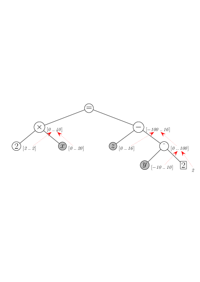
(a) Forward sweep

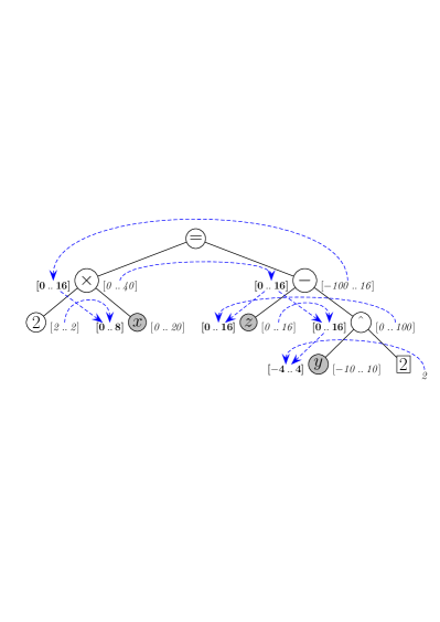
(b) Backward sweep

Figure 1: HC4revise on the constraint $2x=z-y^{2}$

Given the constraint set $\Delta_{C}=\{2x=\alpha_{1},y^{2}=\alpha_{2},z-\alpha_{2}=\alpha_{3},\alpha_{1}=\alpha_{3}\}$ obtained by decomposing $C$ into primitives, it is straightforward to show that HC4revise simply applies all the ReviseBounds procedures in $\Delta_{C}$ in a specific order—induced by the expression tree of $C$—noted $\omega_{C}$ in the sequel.

To be more specific, HC4revise first applies the ReviseBounds procedure for the right-hand variable of all the primitives up to the root, and then the ReviseBounds procedures for the left-hand variables:

$$\mathrm{\mathop{HC4revise}}(C,D)=\\ \hskip 11.38109pt\begin{array}[]{lllll}1.&\text{ReviseBounds}(2x=\alpha_{1},D,\alpha_{1})&\text{\hbox to2.84526pt{}}&6.&\text{ReviseBounds}(2x=\alpha_{1},D,x)\\ 2.&\text{ReviseBounds}(y^{2}=\alpha_{2},D,\alpha_{2})&&7.&\text{ReviseBounds}(z-\alpha_{2}=\alpha_{3},D,z)\\ 3.&\text{ReviseBounds}(z-\alpha_{2}=\alpha_{3},D,\alpha_{3})&&8.&\text{ReviseBounds}(z-\alpha_{2}=\alpha_{3},D,\alpha_{2})\\ 4.&\text{ReviseBounds}(\alpha_{1}=\alpha_{3},D,\alpha_{3})&&9.&\text{ReviseBounds}(y^{2}=\alpha_{2},D,y)\\ 5.&\text{ReviseBounds}(\alpha_{1}=\alpha_{3},D,\alpha_{1})\\ \end{array}$$

Note that, so doing, the domain of each fresh variable introduced by the decomposition process is set to a useful value before being used in the computation of the domain of any other variable.

For admissible constraints, the HC4revise algorithm can be implemented using the DBC algorithm by considering two well-chosen partitions of the set of variables of the decomposed problem. Non-admissible constraints need being made admissible by adding new variables to replace multiple occurrences. The partitioning scheme is given by tree traversals as follows: The first partition $\Gamma$ is obtained by a right-to-left preorder traversal of the tree where visiting a node has the side effect of computing the set of variables associated with its children. The underlying strict partial ordering of the variables is such that a child is greater than its parent. The second partition $\Gamma^{\prime}$ is obtained by inverting the partition computed by a left-to-right preorder traversal of the tree where the visit of a root node associated with a variable $x$ just computes the set $\{x\}$. The underlying strict partial ordering is such that a child is smaller than its parent. HC4revise is equivalent to applying DBC on $\Gamma$ and then on $\Gamma^{\prime}$.

Going back to our example, let us consider the CSP $P=(V,D,\Delta_{C})$, with $V=\{x,y,z,\alpha_{1},\alpha_{2},\alpha_{3}\}$, $D=D[x]\times D[y]\times D[z]\times D[\alpha_{1}]\times D[\alpha_{2}]\times D[\alpha_{3}]$, and $\Delta_{C}$ defined as above. Let us also consider a dummy fresh variable $\alpha_{0}$ supposed to be in the scope of the constraint represented by the root node and its children ($\alpha_{1}=\alpha_{3}$), which is only introduced to initialize the computation of projections. The partitions used to apply HC4revise on $P$ by using Alg. DBC are then as follows:

$$\left\{\begin{array}[]{rcl}\Gamma&=&\{\alpha_{0}\},\{\alpha_{1},\alpha_{3}\},\{z,\alpha_{2}\},\{y\},\{x\}\\ \Gamma^{\prime}&=&\{y\},\{\alpha_{2}\},\{z\},\{\alpha_{3}\},\{x\},\{\alpha_{1}\},\{\alpha_{0}\}\\ \end{array}\right.$$

Let $\gamma_{C}$ (resp. $\gamma^{\prime}_{C}$) be the partial ordering induced by $\Gamma$ (resp. $\Gamma^{\prime}$) on the variables. With its two sweeps on a tree-shaped constraint network, HC4revise appears very similar to Dechter’s ADAPTIVE-TREE-CONSISTENCY algorithm [5, p. 265]. More importantly, the constraint network processed by Alg. DBC being a tree, we can state a result analogous to the one stated by Freuder [7] for arc consistency, which says that, on tree-shaped constraint networks, a bottom-up sweep followed by a top-down sweep are all it takes to enforce bounds consistency:

Proposition 2 (Consistency enforced by HC4revise)

Given $C$ a constraint and $D$ a Cartesian product of domains for the variables in $S[C]$, let $\Delta_{C}$ be the set of primitive constraints obtained by decomposing $C$. We have:

1. $\Delta_{C}$ is directional bounds consistent w.r.t. $\gamma^{\prime}_{C}$ and $D^{\prime\prime}=\mathrm{\mathop{HC4revise}}(C,D)$;

2. if $C$ is an admissible constraint, the constraint system represented by $\Delta_{C}$ is bounds consistent w.r.t. $D^{\prime\prime}=\mathrm{\mathop{HC4revise}}(C,D)$.

Proof

Let $\Gamma$ and $\Gamma^{\prime}$ be two partitions for the variables in $V=\bigcup_{C^{\prime}\in\Delta_{C}}S[C^{\prime}]$ defined as described above. As stated previously, we have $\mathrm{\mathop{HC4revise}}(C,D)=\mathrm{\mathop{DBC}}(\langle V,D^{\prime},\Delta_{C}\rangle,\gamma^{\prime}_{C},\Gamma^{\prime})$, where $D^{\prime}=\mathrm{\mathop{DBC}}(\langle V,D,\Delta_{C}\rangle,\gamma_{C},\Gamma)$.

The first point follows directly from this identity. To prove the second point, let us consider the set $\Pi_{C}$ of projection operators implementing the ReviseBounds procedures for the primitives in $\Delta_{C}$. The HC3 algorithm applied on $\Delta_{C}$ and $D$ would compute the greatest common fixed-point $\top$ included in $D$ of these operators, which is unique since they all are monotonous [3]. By design of HC3, $\Delta_{C}$ is bounds consistent w.r.t. $\top$.

Consider now HC4revise called on $C$ and $D$, which applies each of the operators in $\Pi_{C}$ once in the order $\omega_{C}$:

• either it computes a fixed-point of $\Pi_{C}$, which must be the greatest fixed-point $\top$, by unicity of the gfp and by contractance of the operators in $\Pi_{C}$,

• or, it is possible to narrow further the domains of the variables by applying one of the operators in $\Pi_{C}$. Let $\pi_{1}\colon\beta_{1}\leftarrow f_{1}(\beta_{2},\dots,\beta_{k})$ be this operator. Consider the case where $\pi_{1}$ is an operator applied during the bottom-up sweep. According to the order $\omega_{C}$, $\pi_{2}\colon\beta_{2}\leftarrow f_{2}(\beta_{1},\beta_{3},\dots,\beta_{k}),\dots,\allowbreak\pi_{k}\colon\beta_{k}\leftarrow f_{k}(\beta_{1},\dots,\beta_{k-1})$ have then been applied during the top-down sweep, that is, after having applied $\pi_{1}$. The constraint $C$ being admissible by hypothesis, each variable occurs in only one node in the tree, and then, $\beta_{2},\dots,\beta_{k}$ cannot have been modified after having applied $\pi_{2},\dots,\pi_{k}$. Consequently, reapplying $\pi_{1}$ after the two sweeps cannot narrow down $\beta_{1}$ further, since its most up-to-date value has already been used to compute the current domains for $\beta_{2},\dots,\beta_{k}$ and $\pi_{1}$ is idempotent [3]. We may then conclude that no operator applied during the bottom-up sweep needs to be reapplied. We can use the same arguments for an operator $\pi_{1}$ that was first applied during the top-down sweep.

  As a consequence, no operator in $\Pi_{C}$ needs being reapplied, which contradict our hypothesis that we had not reached a fixed-point. As said above, if HC4revise computes a fixed-point, it is necessarily the greatest common fixed-point $\top$ included in $D$ of the operators in $\Pi_{C}$, and then bounds consistency has been enforced on $\Delta_{C}$.∎

4 Theoretical Analysis of HC4 vs. HC3

The experimental results given in Benhamou et al.’s paper [1] as well as in Section 5 below clearly exhibit the superiority of HC4 versus HC3 to solve large constraint problems. We present in this section the theoretical analysis of these two algorithms.

4.1 Applying HC3 and HC4 to One Constraint Only

In this section as well as in the next, we will consider the projection of a primitive constraint onto a variable as the atomic instruction whose count will serve to characterize the efficiency of the algorithms analyzed.

Let us determine the number of projections to apply in the worst case to enforce bounds consistency on a single admissible constraint (not necessarily primitive). Given a constraint $C$ and its decomposition $\Delta_{C}$ into $p$ primitives, let $k$ be the maximum arity of $\Delta_{C}$ defined by $k=\max_{C^{\prime}\in\Delta_{C}}\text{arity}(C^{\prime})$.

Let $o$ be the number of nodes in the expression tree of $C$. It is easy to observe that $o$ and $p$ are of the same order (more precisely, we have $o/p\sim k$).

Proposition 3 (Worst-case for HC4 on one constraint)

HC4 enforces bounds consistency on the system $\Delta_{C}$ of constraints originating from an admissible constraint $C$ that is decomposable into $p$ primitives in $O(p)$ projections.

Proof

As stressed in the previous section, the tree-shaped constraint network composed naturally by the constraints in $\Delta_{C}$ implies that HC4 will enforce bounds consistency on $\Delta_{C}$ once its two sweeps complete. The number of projections applied is then equal to the $p$ evaluations during the forward sweep plus the projections on the remaining variables for each primitive constraint during the backward sweep, that is at most $(k-1)p$. Overall, the number of projections for HC4revise to enforce bounds consistency is then at most $p+(k-1)p=kp$ projections. ∎

Proposition 4 (Worst-case for HC3 on one constraint)

HC3 enforces bounds consistency on the system $\Delta_{C}$ of constraints originating from an admissible constraint $C$ that is decomposable into $p$ primitives in $O(p^{2})$ projections.

Proof

From Prop. 2, we know that bounds consistency is obtained when the information represented by the domain of each variable (both the user’s ones as well as the fresh ones introduced by the decomposition process) is passed to all the other variables in the tree of $C$. An efficient way to do that indeed corresponds to Alg. HC4revise. Since the tree contains at most $o$ variables, there are at most $o(o-1)$ informations to exchange. Considering an algorithm like BOUNDS-CONSISTENCY, each time a primitive is considered, at least one information is transfered from one variable to the others in its scope (which does not imply necessarily any modification in the associated domains). We then obtain at most $o(o-1)$ calls to primitives. Using the fact that $o$ and $p$ are related by $k$, and that each primitive requires applying at most $k$ projections, with $k$ a constant, the result follows.∎

Relating the worst-cases for HC3 and HC4, we obtain that the ratio $\text{HC3}/\text{HC4}$ is of order $p$ for one constraint in the worst case.

4.2 Applying HC3 and HC4 on a Constraint System

Given a system $R$ of $m$ admissible constraints on $n$ variables $x_{1},\dots,x_{n}$, let $d$ be the size of the largest initial domain. Given $\Delta_{R}$ the constraint system obtained from decomposing the constraints in $R$ into primitives, let $k$ be the maximum arity of $\Delta_{R}$.

As said before, Alg. HC4 enforces bounds consistency on $\Delta_{R}$ by applying Alg. DIRECTIONAL-BOUNDS-CONSISTENCY on each constraint in $R$ twice every time. We stress again that bounds consistency is eventually computed only because we consider admissible constraints in $R$, that is, constraints containing no variable occurring more than once.

Proposition 5 (Worst-case for HC4)

The number of projections to apply to achieve bounds consistency with HC4 on a constraint system $\Delta_{R}$ obtained from a set $R$ of $m$ admissible constraints on $n$ variables is of the order $O(mndp)$ in the worst case.

Proof

The number of constraints to consider is $m$; as shown in Prop. 3, the cost to apply HC4revise is of the order $O(p)$, with $p$ the maximum number of primitives necessary to decompose each constraint in $R$. The result then follows directly from Prop. 1. ∎

Proposition 6 (Worst-case for HC3)

The number of projections to apply to achieve bounds consistency with HC3 on a constraint system $\Delta_{R}$ obtained from a set $R$ of $m$ admissible constraints on $n$ variables is of the order $O(mpd)$ in the worst case.

Proof

First, we must note that the number of constraint to consider is no longer $m$ but at most $mp$, since each constraint has to be decomposed beforehand. The maximum cost of applying HC3revise on a constraint is $k$ (we apply each projection once). Each constraint can only be reinvoked at most $kd$ times. Using Prop. 1, we obtain a worst-case estimate of $mpkdk$, with $k$ a constant. ∎

Relating the costs of computing bounds consistency with either HC4 or HC3, we now obtain $HC3/HC4\sim mpd/(mndp)$, that is, $HC3/HC4\sim 1/n$, which means that the relation is now inverted compared with the case of one admissible constraint only. We then have that the ratio $HC4/HC3$ is of the order of the number of variables in the problem in the worst-case. As we will see in the next section, this pessimistic result is contradicted by all experimental results. It is however easy to get an intuitive understanding of it if one considers that, in the worst case, HC4revise may be called for a constraint each time only one value is removed from the domains of the variables in its scope. Using HC4revise leads to considering $p$ times less constraints than with HC3revise, since the original constraints do not have to be decomposed. However, HC4revise is $p$ times more costly to apply than HC3revise. Overall, HC4 is then penalized by the number of opportunities to reinvoke HC4revise, of the order $nd$ (vs. $kd$ for HC3revise in HC3). Note also that, considering Prop. 6 for a system of only one constraint, we obtain that the number of projections to apply is of the order $O(pd)$ vs. $O(p^{2})$ if we consider Prop. 4. This contradiction is only apparent since, if $d<p$, the $O(p^{2})$ result is clearly pessimistic since it is not possible to apply $p^{2}$ projections (there are not enough values to discard overall), and if $d>p$, $O(pd)$ is pessimistic since at most $p^{2}$ calls suffice to broadcast the information contained by each node in the tree-shaped network of the constraint.

5 Experimental Results

We present the results of both HC4 and HC3 on four standard benchmarks from the interval constraint community. They were chosen so as to be scalable at will and to exhibit various behaviours of the algorithms. As a side note, it is important to remember that these algorithms are often outperformed by other algorithms. Their study is still pertinent, however, since they serve as basic procedures in these more efficient algorithms.

It is important to note also that, originally, none of these problems is admissible. In order to show the impact of admissibility, we have factorized the constraints of one of them.

All the problems have been solved on an AMD Athlon 900 MHz under Linux, using a C++ interval constraint library written for our tests based on the gaol interval arithmetic library. In order to avoid any interference, no optimization (e.g., improvement factor) was used.

For each benchmark, four different methods have been used:

• HC3, which enforces bounds consistency on the decomposed system;

• HC3sb, which uses S-boxes [8]: each user constraint $C$ is decomposed into a separate set of primitives and gives rise to a $\mathrm{\mathop{ReviseBounds}}$ procedure $RB_{C}$ that enforces bounds consistency on this set by using HC3revise procedures for each primitive, and propagating modifications with Alg. 1. All the $RB_{C}$ methods for the constraints in the user system are then handled themselves by Alg. 1. This propagation scheme forces consistency to be enforced locally for each user constraint before reconsidering the others;

• HC4, which enforces a directional bounds consistency (and not bounds consistency, since the constraints are not admissible) on each constraint using HC4revise, and which uses Alg. 1 for the propagation over the constraints in the system;

• HC4sb, which uses one S-box per user constraint. As a consequence, HC4revise is called as many times as necessary to reach a fixed-point for any non-admissible constraint.

Each graphics provided (see Fig. 2) displays the computation time in seconds required to find all solutions up to an accuracy of $10^{-8}$ (difference between the lower and upper bounds of the intervals) for each method.

The bratu constraint system modelizes a problem in combustion theory. It is a square, sparse and quasi-linear system of $n+2$ equations:

$$\left\{\begin{array}[]{l}\forall k\in\{1,\dots,n\}\colon x_{k-1}-2x_{k}+x_{k+1}+\exp(x_{k})/(n+1)^{2}=0,\\ x_{0}=x_{n+1}=0,\\ \forall i\in\{1,\dots,n\}\colon x_{i}\in[-10^{8},10^{8}]\end{array}\right.$$

The largest number of nodes per constraint is independent of the size of the problem and is equal to 12 in our implementation.

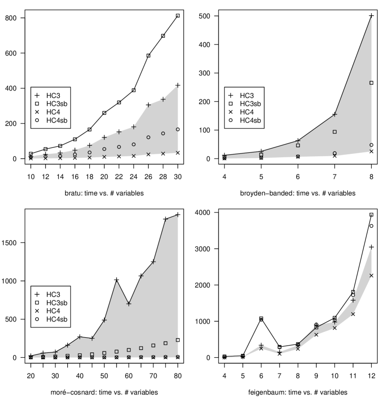
Figure 2: Solving times in seconds for all benchmarks

As already reported by Benhamou et al. [1], HC4 appears more efficient than HC3 to solve all instances of the problem, and its advantage grows with their size. Localizing the propagation does not seem a good strategy here, since HC3sb and HC4sb both perform poorly in terms of the number of projections computed. Interestingly enough, HC4sb is faster than HC3 while it requires more projections. The first reason for this discrepancy that comes to mind is that the “anarchic” propagation in HC3 has a cost much higher in terms of management of the set of constraints to reinvoke than the controlled propagation achieved with HC4sb (see below for another analysis).

The broyden-banded problem is very difficult to solve with HC3, so that we could only consider small instances of it:

$$\begin{array}[]{ll}\forall k\in\{1,\dots,n\}\colon&x_{k}(2+5x_{k}^{2})+1-\sum_{j\in J_{k}}x_{j}(1+x_{j})=0\\ &\text{with }J_{k}=\{j\mid j\neq k\ \wedge\max(1,i-5)\leqslant j\leqslant\min(n,i+1)\},\\ &x_{k}\in[-10^{8},+10^{8}]\\ \end{array}$$

Contrary to bratu, the number of nodes in the constraints is not independent of the size of the problem. It follows however a simple pattern and it is bounded from below by $16$ and from above by $46$.

As with bratu, the efficiency of HC4 compared to HC3 is striking, even on the small number of instances considered. Note that, here, HC3sb is better than HC3. On the other hand, HC4 is still better than HC4sb.

The moré-cosnard problem is a nonlinear system obtained from the discretization of a nonlinear integral equation:

$$\forall k\in\{1,\dots,n\}\colon\left\{\begin{array}[]{l}x_{k}\in[-10^{8},0],\\ x_{k}+\frac{1}{2}[(1-t_{k})\sum_{j=1}^{k}t_{j}(x_{j}+t_{j}+1)^{3}\\ \text{\hbox to28.45274pt{}}+t_{k}\sum_{j=k+1}^{n}(1-t_{j})(x_{j}+t_{j}+1)^{2}]=0\end{array}\right.$$

The largest number of nodes per constraint grows linearly with the number of variables in the problem.

HC4 allows to solve this problem up to 1000 times faster than HC3 on the instances we tested. An original aspect of this benchmark is that localizing the propagation by using S-boxes seems a good strategy: HC3sb solves all instances almost as fast as HC4 (see the analysis in the next section). Note that, once again, though the number of projections required for HC3sb is almost equal to the one for HC4, there is still a sizable difference in solving time, which again might be explained by higher propagation costs in HC3sb.

Lastly, the Feigenbaum problem is a quadratic system:

$$\left\{\begin{array}[]{l}\forall k\in\{1,\dots,n\}\colon x_{k}\in[0,100],\\ \forall k\in\{1,\dots,n-1\}\colon-3.84x_{k}^{2}+3.84x_{k}-x_{k+1}=0,\\ -3.84x^{2}_{n}+3.84x_{n}-x_{1}=0\end{array}\right.$$

The largest number of nodes per constraint is independent of the size of the problem. It is equal to 10 in our implementation.

The advantage of HC4 over HC3 is not so striking on this problem. HC4sb and HC3sb do not fare well either, at least if we consider the computation time.

Parenthetically, the equations in the feigenbaum problem can easily be factorized so that the resulting problem is only composed of admissible constraints. Due to lack of space, the corresponding graphics is not presented here; however, we note that the solving time is reduced by a factor of more than 500 compared to the original version.

6 Discussion

Benhamou et al. [1] have tested the HC4 algorithm on many standard benchmarks. They have shown on each of them the superiority of HC4 over HC3. From the results presented in the preceding section, we have to draw the same conclusions, and to reject entirely the pessimistic view conveyed by our theoretical analysis.

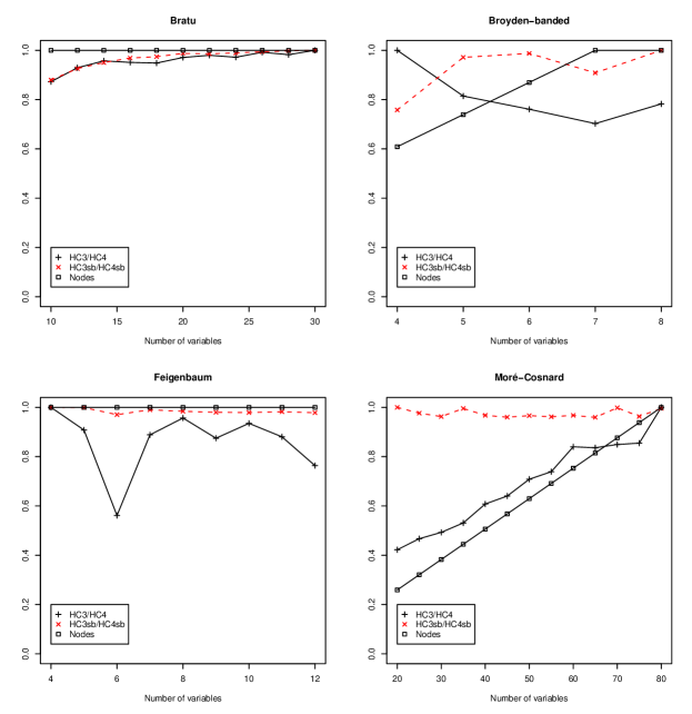
Figure 3: Impact of the number of nodes per constraint on the number of projections

To sum up what has been observed in Section 5, it appears that it is more efficient to deal locally with the modification of a domain induced by some primitive by first reinvoking the other primitives coming from the decomposition of the same user constraint in problems with large constraints like moré-cosnard, while the opposite is true with systems of small constraints such as feigenbaum or bratu. An intuitive understanding of that may be that the information just obtained by a reduction is spread and lost in a large network of primitives while it could be efficiently used locally to compute projections on a user constraint. Figure 3 relates the ratio of the number of projections required by HC3 and HC4, and by HC3sb and HC4sb to the number of nodes in a constraint. As one may see, the ratio is roughly constant for HC3 and HC4 when the number of nodes is independent of the size of the problem, while it increases sharply when the number of nodes increases with the size of the problem (e.g., moré-cosnard). On the other hand, the ratio between HC3sb and HC4sb stays constant for all problems, a fact particularly striking with moré-cosnard. It seems a solid evidence that localization of the information as obtained from using HC4 (or, to a lesser extent, HC3sb), is a winning strategy the larger the constraints in a problem are.

Note however that HC4 is always more efficient than HC4sb on all the benchmarks considered. This is consistent with facts long known by numerical analysts: we show in a paper to come that HC4 may be considered as a free-steering nonlinear Gauss-Seidel procedure where the inner iteration is obtained as in the linear case. For this class of methods, it has been proved experimentally in the past that it is counterproductive to try to reach some fixed-point in the inner iteration.

Benhamou et al. have shown that one successful strategy to solve difficult problems is to make HC4revise cooperate with the revise procedure used to enforce box consistency. A promising direction for future researches is to investigate other cooperation schemes based on the analysis of the structure of the constraints (linear, quadratic, polynomial, …) and of the constraint system (full, banded, …), using the cooperation framework presented by Granvilliers and Monfroy [9] as a basis.

For the interested reader, all the data used to prepare the figures in Section 5 and many more are available in tabulated text format at http://www.sciences.univ-nantes.fr/info/perso/permanents/goualard/dbc-data/.

References

- [1] F. Benhamou, F. Goualard, L. Granvilliers, and J.-F. Puget. Revising Hull and Box Consistency. In Procs. of ICLP ’99, pages 230–244. The MIT Press, 1999.
- [2] F. Benhamou, D. McAllester, and P. Van Hentenryck. CLP(Intervals) revisited. In Procs. of ILPS ’94, pages 124–138. The MIT Press, November 1994.
- [3] F. Benhamou and W.J. Older. Applying interval arithmetic to real, integer and boolean constraints. JLP, 32(1):1–24, 1997.
- [4] E. Davis. Constraint propagation with interval labels. A.I., 32:281–331, 1987.
- [5] R. Dechter. Constraint Processing. Morgan Kaufmann, 1st edition, 2003.
- [6] R. Dechter and J. Pearl. Network-based heuristics for constraint satisfaction problems. A.I., 34:1–38, 1987.
- [7] E.C. Freuder. A sufficient condition for backtrack-free search. J. ACM, 29(1):24–32, 1982.
- [8] F. Goualard and F. Benhamou. A visualization tool for constraint program debugging. In Procs. of ASE ’99, pages 110–117. IEEE Computer Society, 1999.
- [9] L. Granvilliers and É. Monfroy. Implementing Constraint Propagation by Composition of Reductions. In Procs. of ICLP ’03, pages 300–314. Springer, 2003.
- [10] O. Lhomme. Consistency techniques for numeric CSPs. In Procs. of IJCAI ’93, pages 232–238. IEEE Computer Society Press, 1993.
- [11] A.K. Mackworth. Consistency in networks of relations. A.I., 1(8):99–118, 1977.
- [12] F. Messine. Méthodes d’optimisation globale basées sur l’analyse d’intervalle pour la résolution de problèmes avec contraintes. PhD thesis, IRIT, 1997.
- [13] U. Montanari. Networks of constraints: Fundamental properties and applications to picture processing. Information Science, 7(2):95–132, 1974.
- [14] R.E. Moore. Interval Analysis. Prentice-Hall, 1966.
- [15] D.L. Waltz. Understanding line drawings of scenes with shadows. In The Psychology of Computer Vision, chapter 2, pages 19–91. McGraw-Hill, 1975.