Using Self-Organising Mappings to Learn the Structure of Data Manifolds

Abstract: In this paper it is shown how to map a data manifold into a simpler form by progressively discarding small degrees of freedom. This is the key to self-organising data fusion, where the raw data is embedded in a very high-dimensional space (e.g. the pixel values of one or more images), and the requirement is to isolate the important degrees of freedom which lie on a low-dimensional manifold. A useful advantage of the approach used in this paper is that the computations are arranged as a feed-forward processing chain, where all the details of the processing in each stage of the chain are learnt by self-organisation. This approach is demonstrated using hierarchically correlated data, which causes the processing chain to split the data into separate processing channels, and then to progressively merge these channels wherever they are correlated with each other. This is the key to self-organising data fusion.

1 Introduction

The aim of this paper is to illustrate an approach that maps raw data into a representation that reveals its internal structure. The raw data is a high-dimensional vector of sample values output by a sensor such as the samples of a time series or the pixel values of an image, and the representation is typically a lower dimensional vector that retains some or all of the information content of the raw data. There are many ways of achieving this type of data reduction, and this paper will focus on methods that learn from examples of the raw data alone.

A key approach to data reduction is the self-organising map (SOM) [1]. There are many variants of the SOM approach which may be used to map raw data into a lower dimensional space that retains some or all of its information content. In order to increase the variety of mappings SOMs can learn some of these variants use quite sophisticated learning algorithms. For instance, the  topology of a SOM can be learnt by the neural gas approach [2], or the topology of the network connecting several SOMs can be learnt by the growing hierarchical self-organising map (GHSOM) approach [3].

The approach used in this paper aims to achieve a similar type of result to the GHSOM approach. GHSOM is a top-down coarse-to-fine approach to optimising a tree structured network of SOMs, whereas in this paper a bottom-up fine-to-coarse approach will be used that learns a tree structure where appropriate. The choice of a fine-to-coarse rather than coarse-to-fine approach is made in order to obtain networks that can be readily applied to data fusion problems, where the goal is to progressively discard noise (and irrelevant degrees of freedom) as the data passes along the processing chain, thus gradually reducing its dimensionality to eventually obtain a low-dimensional representation of the original raw data.

The basis for the approach used in this paper is a Bayesian theory of SOMs [4] in which a SOM is modelled as an encoder/decoder pair, where the decoder is the Bayes inverse of the encoder. In this approach the encoder is modelled as a conditional probability over all possible codes given the input, and the code that is actually used is a single sample drawn from this conditional probability (i.e. a winner-take-all code). When the conditional probability is optimised to minimise the average Euclidean distortion between the original input and its reconstruction this leads to a network that has properties very similar to a Kohonen SOM.

The basic approach [4] needs to be extended in two separate ways [5]. Firstly, to encourage the self-organisation of a processing chain leading from raw data to a higher level representation, the single encoder/decoder is extended to become a Markov chain of connected encoders, where each encoder feeds its output into the next encoder in the chain. Secondly, to encourage the self-organisation of each encoder into a number of separate smaller encoders and thus to learn tree-structured networks where appropriate, each encoder is generalised to use codes that make simultaneous use of several samples from the conditional probability rather than only a single winner-take-all sample.

The goal of the approach used in this paper is similar to that of the multiple cause vector quantisation approach [6], because the common aim is to split data into its separate components (or causes). However, the approach used in this paper aims to minimise the amount of manual intervention in the training of the network, and thus allow the structure of the data to determine the structure of the network. This is made possible by using codes that consist of several samples from a single conditional probability, which allows each encoder to decide for itself how to split into a number of separate smaller encoders. Also the approach used in this paper does not make explicit use of a generative model of the data, because the aim is only to map raw data into a representation that clarifies its internal structure (i.e. build a recognition model), for which a generative model may be sufficient but is actually not necessary.

This paper is organised as follows. In Section 2 the structure of data is represented as smooth curved manifolds, and encoders are represented as hyperplanes that slice through these manifolds. In Section 3 the theory of a single encoder is developed by extending a Bayesian theory of SOMs [4] from winner-take-all encoders to multiple output encoders, and this theory is further extended to Markov chains of connected encoders [5]. In Section 4 these results are used to train a network on some hierarchically correlated data to demonstrate the self-organisation of a tree-structured network for processing the data.

2 Data Manifolds

In order to represent the structure of data a flexible framework needs to be used. In this paper an approach will be used in which the structure of the data manifold is of primary importance, and the aim is to split apart the manifold in such a way as to reveal how its overall structure is composed. This approach must take account of the relative amplitude of the various contributions, so that a high resolution representation would include even the smallest amplitude contributions to the manifold, and a low resolution representation would retain only the largest amplitude contributions. More generally, it would be useful to construct a sequence of representations, each with a lower resolution than the previous one in the sequence. This could be achieved by progressively discarding the smallest degree of freedom to gradually lower the resolution of the representation. In effect, the representation will become increasingly abstract as it becomes more and more invariant to the fine details of the original data manifold.

In Section 2.1 the basic notation used to describe manifolds is presented, and in Section 2.2 the process of splitting a manifold into its component pieces and then reassembling these to form an approximation to the manifold is described.

2.1 Representation of Data Manifolds

Assume that the raw data vector $x$ lies on a smooth manifold $x(u)$, parameterised by $u$ which is a vector of co-ordinates in the manifold. Usually, though not invariably, $x$ is a high-dimensional vector (e.g. an image comprising an array of pixel values) and $u$ is a low-dimensional vector (e.g. a vector of object positions), in which case the space in which $x$ lives is a high-dimensional embedding space for a low-dimensional manifold. Typically, $u$ represents the underlying degrees of freedom (e.g. object co-ordinates), whereas $x$ represents the observed degrees of freedom (e.g. sensor measurements). Usually, $u$ will contain some noise degrees of freedom, but these can be handled in exactly the same way as other degrees of freedom by splitting $u$ as $u=(u_{s},u_{n})$ where $u_{s}$ is signal and $u_{n}$ is noise. The probability density function (PDF) $\Pr(u)$ describes how the manifold is populated and $\Pr(x)$ (where $\Pr(x)=\int du\Pr(u)\delta(x-x(u))$) describes how the embedding space is populated.

In general, $x(u)$ is a non-linear function of $u$ so the manifold is curved, and thus occupies more linear dimensions of the embedding space than would be the case if the manifold were not curved. It is commonplace for a 1-dimensional manifold (i.e. $u$ is a scalar) to be curved so as to occupy all of the linear dimensions of the embedding space (e.g. the manifold of images generated by moving an object along a 1-dimensional line of positions).

Figure 1: Examples of manifolds generated by images of a pair of objects. In each of the two diagrams the upper half shows the sensor data, and the lower half shows the low-dimensional manifold topology assuming that the sensor data have circular wraparound. The high-dimensional manifold geometry has a number of dimensions equal to the number of pixels in the corresponding sensor. (a) Tensor product of manifolds: 2-torus topology. This is generated by observing each object using a separate sensor.  (b) Superposition (or mixture) of manifolds: This is generated by observing both objects using the same sensor, so that there is the possibility of overlap (possibly with obscuration) of the sensor data from the two objects. In the limit where the objects overlap infrequently case (b) closely approximates case (a).

If $x(u)$ can be written as $x(u)=(x_{1}(u_{1}),x_{2}(u_{2}))$, where $x_{1}(u_{1})$ and $x_{2}(u_{2})$ are independently parameterised manifolds living in separate subspaces of the embedding space (where $\dim x=\dim x_{1}+\dim x_{2}$ and $\dim u=\dim u_{1}+\dim u_{2}$), then $x(u)$ describes a tensor product of manifolds as shown in Figure 1a. This type of manifold arises when the underlying degrees of freedom are measured by separate sensors. This parameterisation can readily be generalised to $x(u)=(x_{1}(u_{1}),x_{2}(u_{2}),\cdots,x_{k}(u_{k}))$ for $k>2$. For independently populated manifolds $\Pr(u)$ factorises as $\Pr(u)=\Pr(u_{1})\Pr(u_{2})$, and if $x(u)=(x_{1}(u_{1}),x_{2}(u_{2}))$ then $\Pr(x)=\Pr(x_{1})\Pr(x_{2})$ where $\Pr(x_{i})=\int du_{i}\Pr(u_{i})\delta(x_{i}-x_{i}(u_{i}))$ for $i=1,2$. For manifolds that are populated in a correlated way (i.e. $\Pr(u)\neq\Pr(u_{1})\Pr(u_{2})$) no such simple result holds.

If $x(u)$ can be written as $x(u)=x_{1}(u_{1})+x_{2}(u_{2})$ (where $\dim x=\dim x_{1}=\dim x_{2}$), then $x(u)$ describes a superposition (or mixture) of manifolds as shown in Figure 1b. This type of manifold arises when the underlying degrees of freedom are simultaneously measured by the same sensor. If there is little or no overlap between $x_{1}(u_{1})$ and $x_{2}(u_{2})$ then this is approximately equivalent to the case $x(u)=(x_{1}(u_{1}),x_{2}(u_{2}))$ (where $\dim x=\dim x_{1}+\dim x_{2}$ and $\dim u=\dim u_{1}+\dim u_{2}$). On the other hand, where there is a significant amount of overlap so that $x_{1}(u_{1}).x_{2}(u_{2})>0$, there is no such correspondence. Assuming $\Pr(u)=\Pr(u_{1})\Pr(u_{2})$ then $\Pr(x)$ is given by $\Pr(x)=\int du_{1}du_{2}\Pr(u_{1})\Pr(u_{2})\delta(x-x_{1}(u_{1})-x_{2}(u_{2}))$.

More generally, $x(u)$ can be written as $x(u)=x(u_{1},u_{2})$ where $x(u_{1},u_{2})$ has no special dependence on $u_{1}$ and $u_{2}$. Although the manifolds are independently parameterised by $u_{1}$ and $u_{2}$, when they are mapped to $x$ their tensor product structure is disguised by the mapping function $x(u_{1},u_{2})$ which is usually not invertible. The superposition of manifolds $x(u)=x_{1}(u_{1})+x_{2}(u_{2})$ is a special case of this effect.

2.2 Mapping of Data Manifolds

Given examples of the raw data $x$ how can an approximation to the mapping function $x(u)$ be constructed? The detailed approach will be described in Section 3,  but the basic geometric ideas will be described here. The basic idea is to cut the manifold into pieces whilst retaining only a limited amount of information about each piece, and then to reassemble these pieces to reconstruct an approximation to the manifold. This process is imperfect because it is disrupted by discarding some of the information about each piece, so the reconstructed manifold is not a perfect copy of the original manifold. This loss of information is critical to the success of this process, because if perfect information were retained then there would be no need to discover a clever way of cutting the manifold into pieces, and thus no possibility of discovering the structure of the manifold (e.g. whether it is a simple tensor product). The information that is preserved depends on exactly how the curved manifold is mapped to a new representation (see Section 3 for details).

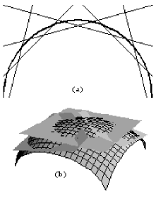
Figure 2: Using hyperplanes to slice pieces off convex curved manifolds. Slicing a curved manifold into pieces prepares it for mapping to another representation. (a) 1-dimensional manifold with arcs being sliced off by chords. (b) 2-dimensional manifold with caps being sliced off by planes (only a few of these are shown in order to keep the diagram simple).

Figure 2a shows an example of how a convex 1-dimensional manifold can be cut into overlapping pieces by a set of lines, and Figure 2b shows the generalisation to the 2-dimensional case. This process is considerably simplified if the manifold is convex because then the hyperplane slices off a localised piece of the manifold, as required.

Figure 3: Manifolds generated by a 1-dimensional object. The data vector is $x=(\cdots,x_{-2},x_{-1},x_{0},x_{1},x_{2},\cdots)$  where $x_{i}=\exp(-\frac{(i-a)^{2}}{2\sigma^{2}})$, $\sigma$ is the width of the object function, $a$ ($-\infty<a<\infty$) is the position of the object, and $i$ ($i=0,\pm 1,\pm 2,\cdots$) is the location of the points where the object amplitude is sampled. The manifolds shown are 3-dimensional embeddings $(x_{1},x_{2},x_{3})$ of the 1-dimensional curved manifolds generated as $a$ varies for a variety of object widths $\sigma$. For $\sigma=0.25$ (i.e. a narrow object function) the manifold is concave with cusps, as $\sigma$ is increased the concavity and the cusps become less pronounced until the manifold crosses the border between being concave and being convex, and for $\sigma=1$ (i.e. a wide object function) the manifold is smoothly convex. Concave manifolds with cusps are not well suited to being sliced apart by hyperplanes whereas smoothly convex manifolds are well suited, and this type of convex manifold is typical of high-dimensional data which also has a high resolution so that each object covers several sample points.

Figure 3 shows an example of how the convexity assumption can break down. The full embedding space contains the vector formed from an array of samples of a 1-dimensional object function, but only three dimensions of the full embedding space are shown in Figure 3. Several scenarios are shown ranging from a narrow object (i.e. undersampled) to a broad object (i.e. oversampled). Oversampling leads to a smooth convex manifold, whereas undersampling leads to a concave manifold with cusps. Typically, convex manifolds occur in signal and image processing where the raw data are sampled at a high enough rate, and non-convex manifolds occur when the raw data has already been processed into a low-dimensional form, such as when some underlying degrees of freedom (or features) have already been extracted from the raw data.

Figure 4: Using a stochastic vector quantiser (SVQ) to map a curved manifold to a new representation (see Section 3 for details). The manifold is the unit circle which is softly sliced up by the SVQ posterior probabilities, which are defined as the (normalised) outputs of a set of sigmoid functions, which in turn depend on a set of weight vectors and biases. For each sigmoid function a dashed line is drawn to show where its (unnormalised) output is $\frac{1}{2}$, although here it is the curved contours of the posterior probabilities (rather than the dashed lines) that are actually used to slice up the manifold.

Figure 4 shows the results obtained by for a circular manifold using the stochastic vector quantiser (SVQ) approach of Section 3. The results correspond to Figure 2a, except that now the slicing is done softly in order to preserve additional information about the manifold, and to ensure that the reconstructed manifold does not show artefacts when the slices are reassembled.

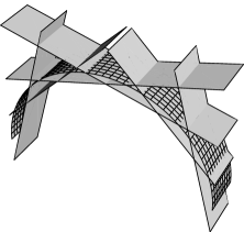
Figure 5: Using hyperplanes to slice pieces off a curved manifold. The manifold is 2-dimensional with a large and a small degree of freedom. Each hyperplane slices through the manifold in such a way that it cuts off a piece of the manifold that has a limited range of values of the large degree of freedom but all possible values of the small degree of freedom. This is the basic means by which a manifold can be mapped to a new representation.

Figure 5 shows an example of how a convex $(1+\epsilon)$-dimensional manifold (a small length extracted from a cylindrical surface) can be cut into overlapping pieces by a set of planes. The 1 in $(1+\epsilon)$ is a large degree of freedom (arc length around the cylinder)), whereas the $\epsilon$ in $(1+\epsilon)$ is a small degree of freedom (length along the cylinder) because it has a small amplitude compared to the large degree of freedom. Because of the orientation of the planes they are insensitive to the small degree of freedom, so the reconstructed manifold is 1-dimensional manifold (i.e. the $\epsilon$ component has been discarded). The orientation of the planes may be used in various ways to control their sensitivity to the manifold, and some quite sophisticated examples of this will be discussed in Section 4. These results generalise to soft slicing as used in Figure 4.

3 Learning a Manifold

In order to learn how to represent the structure of a data manifold a flexible framework needs to be used. In this paper an approach will be used in which the manifold is mapped to a lower resolution representation in such a way that a good approximation to the original manifold can be reconstructed. Key requirements are that these mappings can be cascaded to form sequences of representations of progressively lower resolution having more and more invariance with respect to details in the original manifold, and that the mappings can learn to represent tensor products of manifolds so that the representation of the manifold can split into separate channels. To achieve this it is sufficient to use a variant [5] of the standard vector quantiser [7] to gradually compress the data.

In Section 3.1 the theory of stochastic vector quantisers (SVQ) is presented, and in Section 3.2 it is extended to chains of linked SVQs.

3.1 Stochastic Vector Quantiser

As was discussed in Section 2 a procedure is needed for cutting a manifold into pieces and then reassembling these pieces to reconstruct the manifold. It turns out that all of the required properties emerge automatically from vector quantisers (VQ), and their generalisation to stochastic vector quantisers (SVQ).

Figure 6: A matched encoder/decoder pair represented as a folded Markov chain (FMC) $x_{0}\longrightarrow x_{1}\longrightarrow\overset{~{}}{x}_{1}\longrightarrow\overset{~{}}{x}_{0}$. The input $x_{0}$ is encoded as $x_{1}$ which is then passed along a distortionless communication channel to become $\overset{~{}}{x}_{1}$ which is then decoded as $\overset{~{}}{x}_{0}$. The encoder is modelled using the conditional probability $\Pr(x_{1}|x_{0})$ to allow for the possibility that the encoder is stochastic, and the corresponding decoder is modelled using the Bayes inverse conditional probability $\Pr(\overset{~{}}{x}_{0}|\overset{~{}}{x}_{1})$. The distortionless communication channel is modelled using the delta function $\delta(\overset{~{}}{x}_{1}-x_{1})$.

Figure 6 shows a folded Markov chain (FMC) as described in [4]. An FMC encodes its input $x_{0}$ (i.e. cuts the input manifold into pieces using the conditional PDF $\Pr(x_{1}|x_{0})$) and then reconstructs an approximation to its input $\overset{~{}}{x}_{0}$ (i.e. reassembling the pieces to reconstruct the input manifold using the Bayes inverse PDF $\Pr(\overset{~{}}{x}_{0}|x_{1})=\frac{\Pr(x_{1}|\overset{~{}}{x}_{0})\Pr(\overset{~{}}{x}_{0})}{\Pr(x_{1})}$), so it is ideally suited to the task at hand. An objective function $D$ needs to be defined to measure how accurately the reconstruction $\overset{~{}}{x}_{0}$ approximates the original input $x_{0}$.

It is simplest to use a Euclidean objective function that measures the average squared (i.e. $L^{2}$) distance $\|x_{0}-\overset{~{}}{x}_{0}\|^{2}$, and which must be minimised with respect to the encoder $\Pr(x_{1}|x_{0})$ (note that the decoder $\Pr(\overset{~{}}{x}_{0}|\overset{~{}}{x}_{1})$ is then completely determined by Bayes’ theorem).

$$D=\int dx_{0}dx_{1}d\overset{~{}}{x}_{0}d\overset{~{}}{x}_{1}\Pr(x_{0})\Pr(x_{1}|x_{0})\delta(\overset{~{}}{x}_{1}-x_{1})\Pr(\overset{~{}}{x}_{0}|\overset{~{}}{x}_{1})\left\|x_{0}-\overset{~{}}{x}_{0}\right\|^{2}$$ (1)

Using Bayes’ theorem Equation 1 can be manipulated into the form [4]

$$D=2\int dx_{0}dx_{1}\Pr(x_{0})\Pr(x_{1}|x_{0})\left\|x_{0}-\overset{~{}}{x}_{0}(x_{1})\right\|^{2}$$ (2)

where $D$ must be minimised with respect to both the encoder $\Pr(x_{1}|x_{0})$ and the reconstruction vector $\overset{~{}}{x}_{0}(x_{1})$. Note that this simplification of Equation 1 into Equation 2 depends critically on the Euclidean form of the objective function.

Figure 7: An encoder/decoder pair represented as the chain $x_{0}\longrightarrow x_{1}\longrightarrow\overset{~{}}{x}_{0}(x_{1})$. This contains only those parts of the FMC that affect the Euclidean distortion objective function.

Figure 7 is a transformed version of Figure 6 that reflects the transformation of Equation 1 into Equation 2. The encoder $\Pr(x_{1}|x_{0})$ is the most important part of this diagram, whereas the reconstruction vector $\overset{~{}}{x}_{0}(x_{1})$ is less important so it is shown as a dashed line.

Thus far a non-parametric representation of $\Pr(x_{1}|x_{0})$ and $\overset{~{}}{x}_{0}(x_{1})$ has been used, so analytic minimisation of $D$ [4] leads to $\Pr(x_{1}|x_{0})\longrightarrow\delta(x_{1}-x_{1}(x_{0}))$, in which case the encoder could be perfect (i.e. lossless) and it would not be possible to discover the structure of the input manifold, as discussed in Section 2. To make progress constrained forms of $\Pr(x_{1}|x_{0})$ and $\overset{~{}}{x}_{0}(x_{1})$ must be used in order to limit the resources available to the encoder/decoder, and thus force it to discover clever ways of mapping the input manifold to reduce the damage caused by having only limited coding resources.

One way of constraining the encoder/decoder is for $x_{1}$ to be a scalar index $y_{1}$ where $y_{1}=1,2,\cdots,m_{1}$ ($m_{1}$ is the size of the code book), which is a single sample drawn from the encoder $\Pr(x_{1}|x_{0})$. Analytic minimisation of $D$ [4] now leads to $\Pr(x_{1}|x_{0})\longrightarrow\delta_{y_{1},y_{1}(x_{0})}$ so that $D=2\int dx_{0}\Pr(x_{0})\|x_{0}-\overset{~{}}{x}_{0}(y_{1}(x_{0}))\|^{2}$ which is the objective function for a standard least squares vector quantiser [7].

A better way of constraining the encoder/decoder is for $x_{1}$ to be the histogram $(\nu_{1},\nu_{2},\cdots,\nu_{m_{1}})$ of counts of independent samples of the scalar index $y_{1}$ ($n_{1}=\sum_{y_{1}=1}^{m_{1}}\nu_{y_{1}}$ is the total number of samples), and for $\overset{~{}}{x}_{0}(x_{1})$ to be approximated as $\overset{~{}}{x}_{0}(x_{1})\approx\sum_{y_{1}=1}^{m_{1}}\frac{\nu_{y_{1}}}{n_{1}}\overset{~{}}{x}_{0}(y_{1})$ (rather than using the full functional form $\overset{~{}}{x}_{0}(\nu_{1},\nu_{2},\cdots,\nu_{m_{1}})$). Although it is still possible to obtain analytic results it usually requires a lot of calculation [8], and it is generally better to use a numerical optimisation approach. An upper bound for the objective function $D$ is then given by [9]

$$\begin{array}[]{rl}D&\leq\frac{2}{n_{1}}\int dx_{0}\Pr(x_{0})\sum\limits_{y_{1}=1}^{m_{1}}\Pr(y_{1}|x_{0})\left\|x_{0}-\overset{~{}}{x}_{0}(y_{1})\right\|^{2}\\ &\begin{array}[]{cc}&\end{array}+\frac{2\left(n_{1}-1\right)}{n_{1}}\int dx_{0}\Pr(x_{0})\left\|x_{0}-\sum\limits_{y_{1}=1}^{m_{1}}\Pr(y_{1}|x_{0})\overset{~{}}{x}_{0}(y_{1})\right\|^{2}\end{array}$$ (3)

where the unconstrained encoder/decoder corresponds to the left hand side of Equation 3 and the constrained encoder/decoder corresponds to the right hand side of Equation 3. Note how the random fluctuations in the multiple sample histogram are analytically summed over in Equation 3, leaving only the single sample encoder $\Pr(y_{1}|x_{0})$ to be optimised.

A further constraint is to assume that $\Pr(y_{1}|x_{0})$ is parameterised as the normalised output of a set of sigmoid functions

$$\begin{array}[]{rl}\Pr(y_{1}|x_{0})&=\frac{Q(y_{1}|x_{0})}{\sum_{y_{1}^{\prime}=1}^{m_{1}}Q(y_{1}^{\prime}|x_{0})}\\ Q(y_{1}|x_{0})&=\frac{1}{1+\exp(-w_{10}(y_{1}).x_{0}-b_{1}(y_{1}))}\end{array}$$ (4)

where $Q(y_{1}|x_{0})$ is the unnormalised output from code index $y_{1}$, depending on the weight vector $w_{10}(y_{1})$ and the bias $b_{1}(y_{1})$. This parameterisation of $\Pr(y_{1}|x_{0})$ ensures that it can be used to slice pieces off convex manifolds as illustrated in Figure 4. Optimisation of the objective function is then achieved by gradient descent variation of the three sets of parameters $w_{10}(y_{1})$, $b_{1}(y_{1})$, and $\overset{~{}}{x}_{0}(y_{1})$. These (and other) derivatives of the objective function were given in [9].

The constrained objective function in Equation 3 and Equation 4 yields a great variety of useful results, such as the simple result shown in Figure 4 which used $m_{1}=6$, $n_{1}=20$, and $x_{0}=(\cos\theta,\sin\theta)$ with $\theta$ uniformly distributed in $[0,2\pi]$, to learn a mapping from the 1-dimensional input manifold embeded in a 2-dimensional space ($\dim x_{0}=2$) to a 6-dimensional space ($m_{1}=6$). This is the key objective function that can be used to optimise the mapping of the input manifold to a new representation $\Pr(y_{1}|x_{0})$ for $y_{1}=1,2,\cdots,m_{1}$. Minimising the Euclidean distortion ensures that $\Pr(y_{1}|x_{0})$ defines an optimal mapping of the input manifold, such that when $n_{1}$ samples are drawn from $\Pr(y_{1}|x_{0})$ they contain enough information to form an accurate reconstruction of $x_{0}$.

Figure 8: A factorial encoder/decoder pair represented as the pair of disconnected chains $x_{0}^{a}\longrightarrow x_{1}^{a}\longrightarrow\overset{~{}}{x}_{0}^{a}(x_{1}^{a})$ and $x_{0}^{b}\longrightarrow x_{1}^{b}\longrightarrow\overset{~{}}{x}_{0}^{b}(x_{1}^{b})$. The input vector is $x_{0}=(x_{0}^{a},x_{0}^{b})$ highlighted by the left hand rectangle, the code is $x_{1}=(x_{1}^{a},x_{1}^{b})$ highlighted by the right hand rectangle, and the reconstruction is $\overset{~{}}{x}_{0}=(\overset{~{}}{x}_{0}^{a},\overset{~{}}{x}_{0}^{b})$. The dependencies amongst the variables is indicated by the arrows in the diagram, which shows that subspaces $a$ and $b$ are independently encoded/decoded.

Figure 8 is a transformed version of Figure 7 that shows an example of the structure of some types of optimal solution that are obtained by minimising the constrained objective function in Equation 3. The tensor product structure of the input manifold is revealed in this type of solution, because the input vector $x_{0}$ splits into two parts as $x_{0}=(x_{0}^{a},x_{0}^{b})$ each of which is separately encoded/decoded. This type of factorial encoder is favoured by limiting the size of the code book $m$ and by using an intermediate number of samples $n_{1}$ ($n_{1}=1$ leads to a standard VQ, and $n_{1}\longrightarrow\infty$ allows too many coding resources to lead to clever encoding schemes).

The self-organised emergence of factorial encoders is one of the major strengths of the SVQ approach. It allows the code book to split into two or more separate smaller code books in a data driven way rather than being hard-wired into the code book at the outset (e.g. [6]).

3.2 Chain of Stochastic Vector Quantisers

The encoder/decoder in Figure 7 leads to useful results for mapping the input data manifold when its operation is constrained in various ways. A much larger variety of mappings may be constructed if the encoder/decoder is viewed as a basic module, and then networks of linked modules are used to process the data [5]. It is simplest to regard this type of network as progressively mapping the input manifold as it flows through the network modules.

Figure 9: A 3-stage chain of linked SVQs. The $l^{\textup{th}}$ encoder is modelled using the conditional probability $\Pr_{l,l-1}(x_{l}|x_{l-1})$, and the corresponding decoder is modelled using the reconstruction vectors $\overset{~{}}{x}_{l-1}(x_{l})$, where each $x_{l}$ is a histogram of samples.

Figure 9 shows a 3-stage chain of linked encoder/decoders of the type shown in Figure 7. The important part of this diagram is the processing chain which is the solid line flowing from left to right at the top of the diagram creating the Markov chain $x_{0}\overset{\Pr(x_{1}|x_{0})}{\longrightarrow}x_{1}\overset{\Pr(x_{2}|x_{1})}{\longrightarrow}x_{2}\overset{\Pr(x_{3}|x_{1})}{\longrightarrow}x_{3}$. The reconstruction vectors $\overset{~{}}{x}_{l-1}(x_{l})$ for $l=1,2,3$ are the dashed lines flowing from right to left.

The state $x_{l}$ of layer $l$ of the chain is the histogram $(\nu_{1},\nu_{2},\cdots,\nu_{m_{l}})$ of counts of samples drawn from $\Pr(y_{l}|x_{l-1})$ ($n_{l}=\sum_{y_{l}=1}^{m_{l}}\nu_{y_{l}}$ is the total number of samples). In numerical implementations $x_{l}$ is chosen to be the (normalised) histogram for an infinite number of samples (i.e. the relative frequencies implied by $\Pr(y_{l}|x_{l-1})$), and $\overset{~{}}{x}_{l-1}(x_{l})$ is chosen to depend on only a finite number $m_{l}$ of samples randomly selected from this histogram  $\overset{~{}}{x}_{l-1}(x_{l})\approx\sum_{y_{l}=1}^{m_{l}}\frac{\nu_{y_{l}}}{n_{l}}\overset{~{}}{x}_{l-1}(y_{l})$. This choice of how to operate the network is not unique but it has the advantage of  simplifying the computations. The infinite number of samples used in $x_{l}$ ensures that the $x_{l}$ do not randomly fluctuate, so no Monte Carlo simulations are required to implement the feed-forward flow through the network. The finite number of samples $n_{l}$ used in $\overset{~{}}{x}_{l-1}(x_{l})$ leads to exactly the same objective function as in Equation 3 where the random fluctuations are analytically summed over, which ensures that each decoder has limited resources and thus forces the optimisation of the network to discover intelligent ways of encoding the data. This type of network reduces to a standard way of using a Markov chain when only a single sample is drawn from each of the $\Pr(y_{l}|x_{l-1})$.

Each stage of the chain corresponds to an objective function of the form shown in Equation 3 but applied to the $l^{\textup{th}}$ stage of the chain. The total objective function is a weighted sum of these individual contributions. This encourages all of the mappings in the chain to minimise their average Euclidean reconstruction error, which gives a progressive mapping of the input manifold along the processing chain. However, the relative weighting of the later stages of the chain must not be too great otherwise they force the earlier mappings in the chain to become singular (e.g. all inputs mapped to the same output), because the output of a singular mapping can be mapped with little or no more contribution to the overall objective function further along the chain. A less extreme form of this phenomenon can be used to encourage factorial encoders to emerge, because they produce a (normalised) histogram output state that has a smaller volume (in the Euclidean sense) than a non-factorial encoder, which reduces the size of the contribution to the overall objective function from the next stage in the chain.

If the chain network topology in Figure 9 is combined with the factorial encoder/decoder property of SVQs shown in Figure 8 then all acyclic network topologies are possible. This can be seen intuitively because flow through the chain corresponds to flow along the time-like direction in an acyclic network (i.e. following the directed links), and multiple parallel branches occur wherever there is an SVQ factorial encoder in the chain. An example of the emergence of this type of network topology will be shown in Section 4.

4 Learning a Hierarchical Network

The purpose of this section is to demonstrate the self-organised emergence of a hierarchical network topology starting from a chain-like topology of the type shown in Figure 9. For the purpose of this demonstration the raw data must have an appropriate correlation structure, which will be achieved by generating the data as a set of hierarchically correlated phases. Thus each data vector is a 4-dimensional vector of phases $\phi=(\phi_{1},\phi_{2},\phi_{2},\phi_{4})$, where the $\phi_{i}$ are the leaf nodes of a binary tree of phases, where the binary splitting rule used is $\phi\longrightarrow(\phi-\alpha,\phi+\beta)$ with $\alpha$ and $\beta$ being independently and uniformly sampled from the interval $[0,\frac{\pi}{2}]$, and the phase of the root node is uniformly distributed in the interval $[0,2\pi]$. This will lead to each of the $\phi_{i}$ being uniformly distributed phase variables thus uniformly occupying a circular manifold. However, because the $\phi_{i}$ are correlated due to the way that they are generated by the binary splitting process, the $\phi$ do not uniformly populate a 4-torus manifold (i.e. tensor product of 4 circles).

Figure 5 showed an example of what the manifold of a pair of correlated variables looks like, with a large degree of freedom (e.g. $\phi_{1}+\phi_{2}$) and a small degree of freedom (e.g. $\phi_{1}-\phi_{2}$), and the hyperplanes encoding the manifold in such a way as to discard information about the small degree of freedom (e.g. $\phi_{1}-\phi_{2}$). In this way the 3-stage chain in Figure 9 can progressively discard information about small degrees of freedom in $\phi$, starting with a 4-torus manifold (non-uniformly populated) and ending up with a circular manifold (uniformly populated), as will be seen below. This is the basic idea behind using this type of self-organising network for data fusion.

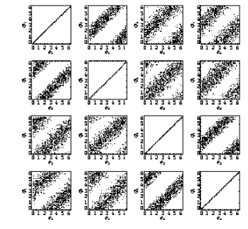
Figure 10: Co-occurrence matrices of all pairs of phases. Note that the block structure is symmetric so each off-diagonal co-occurrence matrix appears twice. The hierarchical correlations cause $\phi_{1}$and $\phi_{2}$  (and similarly $\phi_{3}$ and $\phi_{4}$) to be more strongly correlated with each other than $\phi_{2}$ and $\phi_{3}$.

Figure 10 shows the co-occurrence matrices of pairs of the $\phi_{i}$ displayed as scatter plots. The bands in these plots wrap around circularly and correspond to the manifold shown in Figure 5. Because $\phi_{1}$ and $\phi_{2}$ (and also $\phi_{3}$ and $\phi_{4}$) lie close to each other in the hierarchy, $\Pr(\phi_{1,}\phi_{2})$ and $\Pr(\phi_{3},\phi_{4})$ have a narrower band than $\Pr(\phi_{1,}\phi_{3})$, $\Pr(\phi_{1,}\phi_{4})$, $\Pr(\phi_{2,}\phi_{3})$ and $\Pr(\phi_{2,}\phi_{4})$.

A 3-stage chain of linked SVQs of the type shown in Figure 9 is now trained, where each stage contributes an objective function of the form shown in Equation 3 and Equation 4. The sizes $M$ of each of the 4 network layers are $M=(8,16,8,4)$. The size of layer 0 (the input layer) is determined by the dimensionality of the input data, whereas the sizes of each of the other layers is chosen to be 4 times the number of phase variables that each is expected to use in its encoding of the input data, which encourages the progressive removal of small degrees of freedom from the data as it flows along the chain into ever smaller layers. The number of samples $n$ used for each of the 3 SVQ stages are $n=(20,20,20)$, which are large enough to allow each SVQ to develop into a factorial encoder, so that the processing can proceed in parallel along several paths (which are progressively fused) along the chain. The relative weightings $\lambda$ assigned to the objective functions contributed by each of the 3 SVQ stages are $\lambda=(1,5,0.1)$, where a large weighting is assigned to the stage 2 SVQ to encourage the stage 1 SVQ to develop into a factorial encoder, and a small weighting is assigned to the stage 3 SVQ because the stage 2 SVQ needs no additional encouragement to develop into a factorial encoder.

The network was trained by a gradient descent on the overall network objective function, using a step size chosen separately for each SVQ stage and separately for each of the 3 parameter types $w_{l,l-1}(y_{l})$, $b_{l}(y_{l})$, and $\overset{~{}}{x}_{l-1,l}(y_{l})$ in each SVQ stage (for $l=1,2,3$). The size of all of these step size parameters was chosen to be large at the start of the training schedule, and then gradually reduced as training progressed, with the relative rate of reduction being chosen to encourage earlier SVQ stages to converge before later SVQ stages. In general, different choices of network parameters and training conditions lead to different types of trained network, and since there is no prior reason for choosing one particular solution in preference to another the choice must be left up to the user. All the components of the weight vectors, biases, and reconstruction vectors are initialised to random numbers uniformly distributed in the interval  $[-0.1,0.1]$.

Figure 11: Reconstruction vectors $\overset{~{}}{x}_{l-1,l}(y_{l})$ (for $l=1,2,3$) after training a 3-stage network of linked SVQs on the hierarchically correlated phases data. These diagrams are rotated $90^{\circ}$ anticlockwise relative to Figure 9, so the processing chain runs from bottom to top of each diagram. Line thickness indicates the size of a reconstruction vector component, and dashing indicates that the component is negative. (a) All reconstruction vector components. (b) Largest reconstruction vector components obtained by applying a threshold to the magnitude of each component. (c) The same as (b) except that the positions of the nodes in all layers (other than the input layer) have been permuted (along with the connections between layers) to make the network topology clearer.

Figure 11 shows the reconstruction vectors $\overset{~{}}{x}_{l-1,l}(y_{l})$ (for $l=1,2,3$) in a trained 3-stage chain of linked SVQs of the type shown in Figure 9. Reconstruction vectors are displayed because they are easier to interpret than weight vectors. The data $\phi=(\phi_{1},\phi_{2},\phi_{2},\phi_{4})$ is embedded in an 8-dimensional input space as $x=(x_{1},x_{2},x_{3},x_{4},x_{5},x_{6},x_{7},x_{8})$ where $(x_{2i-1},x_{2i})=(\cos\phi_{i},\sin\phi_{i})$. The key diagram is Figure 11c which shows the largest components of the reconstruction vectors, and has been reordered to make the hierarchical network topology clear. Each of the first two stages of this network has learnt to operate as two or more encoder/decoders (i.e. a factorial encoder/decoder) as in Figure 8. The first stage of the network breaks into 4 encoder/decoders that encode each of the $\phi_{i}$ (see the results in Figure 14 and Figure 15 for justification of this), the second stage of the network breaks into 2 encoder/decoders that encode $\phi_{1}+\phi_{2}$ and $\phi_{3}+\phi_{4}$ (see the results in Figure 16 and Figure 17 for justification of this), and the third stage of the network is a single encoder that encodes $\phi_{1}+\phi_{2}+\phi_{3}+\phi_{4}$ (see the results in Figure 18 and Figure 19 for justification of this). The connectivity in the stage 1 SVQ is not the same for all of the $\phi_{i}$ because of the interaction between the thresholding prescription used to create Figure 11 and the different orientation of each of the 4 parts of the stage 1 factorial encoder with respect to each of the 4 corresponding circular input manifolds.

Although the network in Figure 11 computes using continuous-valued numbers, the thresholded reconstruction vectors in Figure 11b may be inspected to reveal the symbolic logic expressions that approximate to each of the (thresholded) outputs $O_{i}(x)$ for $i=1,2,3,4$ from the highest layer of the network (using logical negation $\overset{\_}{x}_{i}$ to denote $-x_{i}$ because the inputs lie in the range $[-1,1]$).

$$\begin{array}[]{rl}O_{1}(x)&=\overset{\_}{x}_{2}\cap x_{3}\cap x_{5}\cap x_{8}\\ O_{2}(x)&=x_{2}\cap\overset{\_}{x}_{3}\cap\overset{\_}{x}_{5}\cap\overset{\_}{x}_{8}\\ &=\overset{\_}{O}_{1}(x)\\ O_{3}(x)&=\overset{\_}{x}_{1}\cap\overset{\_}{x}_{4}\cap\overset{\_}{x}_{6}\cap x_{7}\\ O_{4}(x)&=x_{1}\cap x_{4}\cap x_{6}\cap\overset{\_}{x}_{7}\\ &=\overset{\_}{O}_{3}(x)\end{array}$$ (5)

In order to keep these expressions short they use a slightly higher threshold than was used to create Figure 11b, because this suppresses some of the reconstruction vector components linked to $(x_{1},x_{2},x_{3},x_{4})$. In this particularly simple example it is possible to obtain very short symbolic expressions, but more generally continuous-valued computations would be needed to obtain good approximations to the  network outputs.

Figure 12: Some typical examples of node activities $\Pr(y_{l}|x_{l-1})$ (for $l=1,2,3$) in the trained 3-stage network of linked SVQs. The permuted version of the network is used to make the results easier to interpret. The area of each filled circle is proportional to the activity it represents, and the negative values that occur in the input layer are represented by unfilled circles. The hierarchical structure of the network is indicated by drawing a box around each part of each network layer that acts as a separate encoder, so that typically there are one or two active nodes within every box.

Figure 12 shows some examples of the node activities $\Pr(y_{l}|x_{l-1})$ (for $l=1,2,3$) in the trained network shown in Figure 11c. The individual pieces of each factorial encoder are indicated by the boxes, and the patterns of activity are such that every box contains one or more active nodes, as would be expected if each box were acting as a separate encoder.

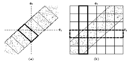
Figure 13: Two ways of encoding a pair of correlated phases $\phi_{1}$ and $\phi_{2}$. The co-occurrence matrix of $\phi_{1}$ and $\phi_{2}$ is represented as a narrow band that is populated by data points, so that the correlation manifests itself as $\phi_{1}\approx\phi_{2}$. (a) This shows how an invariant encoder operates, in which the response region of each node is oriented so that it has high resolution for the $\phi_{1}+\phi_{2}$ but is completely insensitive to $\phi_{1}-\phi_{2}$. This does not encode information about the small degree of freedom measured across the band of the co-occurrence matrix. (b) This shows how a factorial encoder operates, in which the response region of each node is highly anisotropic, with high resolution for one of the phases but completely insensitive to the other phase. Accurate encoding is achieved by using the nodes in pairs with orthogonally intersecting response regions, as shown in the example highlighted in the diagram.

Figure 13 shows simplified versions of the two types of encoder/decoder that occur in Figure 11 overlaid on a co-occurrence matrix of the type shown in Figure 10.

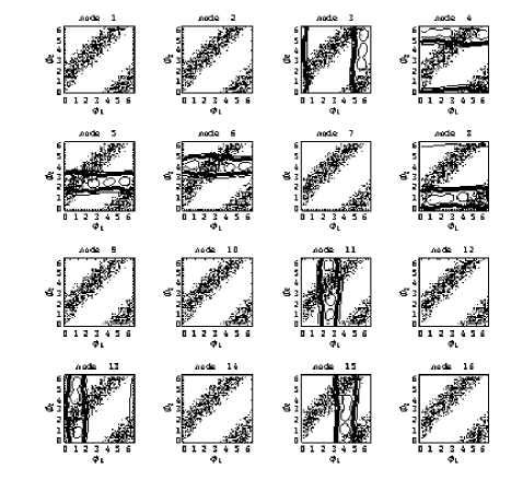
Figure 14: Node activities in layer 1 as a function of the inputs $\phi_{1}$ and $\phi_{2}$ (with $\phi_{3}=\phi_{4}=0$) which has the properties of a factorial encoder. In each plot the contours representing the node reponse are overlaid on the co-occurrence matrix of the pair of inputs $\phi_{1}$ and $\phi_{2}$. One of the contour heights is drawn bold to highlight the region where the node response is large. Half of the nodes do not respond at all, and the other half split into two subsets of equal size, one with high resolution in $\phi_{1}$ but completely insensitive to $\phi_{2}$, and the other with high resolution in $\phi_{2}$ but completely insensitive to $\phi_{1}$.  The response is sensitive to the small degree of freedom measured across the band of the co-occurrence matrix. The non-zero responses correspond to the 8 nodes in layer 1 that are strongly connected to $\phi_{1}$ and $\phi_{2}$.

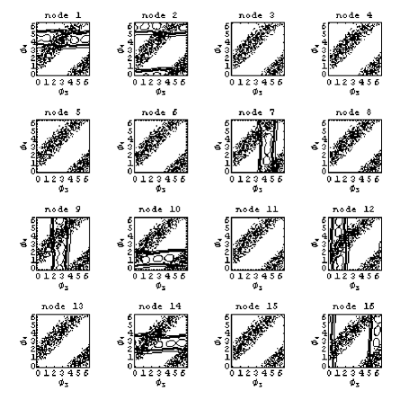
Figure 15: Node activities in layer 1 as a function of the inputs $\phi_{3}$ and $\phi_{4}$ (with $\phi_{1}=\phi_{2}=0$) which has the properties of a factorial encoder. The non-zero responses correspond to the 8 nodes in layer 1 that are strongly connected to $\phi_{3}$ and $\phi_{4}$.

Figure 14 and Figure 15 show the encoders that occur in stage 1 of Figure 11. These are all factorial encoders of the type shown in Figure 13b, as can be seen from the orientation of the response regions for the various nodes which cuts across the band of the co-occurrence matrix in the same way as in Figure 13b. This corresponds to the connectivity seen in Figure 11c where each $\phi_{i}$ has its own encoder.

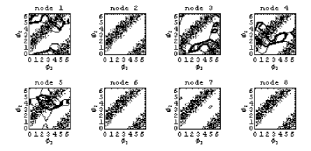
Figure 16: Node activities in layer 2 as a function of the inputs $\phi_{1}$ and $\phi_{2}$ (with $\phi_{3}=\phi_{4}=0$) which has the properties of an invariant encoder. Half of the nodes do not respond at all, and the other half respond to well-defined regions in $\phi_{1}$ and $\phi_{2}$. The contours representing the node response are overlaid on the co-occurrence matrix of the pair of inputs $\phi_{1}$ and $\phi_{2}$. One of the contour heights is drawn bold to highlight the region where the node response is large. This shows that each node responds to a local region of the populated region of the co-occurrence matrix, and to a limited extent generalises outside this region. The response is invariant with respect to the small degree of freedom measured across the band of the co-occurrence matrix, which demonstrates that layer 2 has acquired an invariance that was absent in layer 1. There are also non-zero responses in the unpopulated region of the co-occurrence matrix which arise because the sum of the node activities is normalised. The non-zero responses correspond to the 4 nodes in layer 2 that are strongly connected to $\phi_{1}$ and $\phi_{2}$.

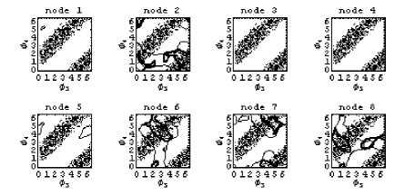
Figure 17: Node activities in layer 2 as a function of the inputs $\phi_{3}$ and $\phi_{4}$ (with $\phi_{1}=\phi_{2}=0$) which has the properties of an invariant encoder. The non-zero responses correspond to the 4 nodes in layer 2 that are strongly connected to $\phi_{3}$ and $\phi_{4}$.

Figure 16 and Figure 17 show the encoders that occur in stage 2 of Figure 11. These are invariant encoders of the type shown in Figure 13a, as can be seen from the orientation of the response regions for the various nodes which cuts across the band of the co-occurrence matrix in the same way as in Figure 13a. This corresponds to the connectivity seen in Figure 11c where each of $\phi_{1}+\phi_{2}$ and $\phi_{3}+\phi_{4}$ has its own encoder.

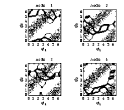
Figure 18: Node activities in layer 3 as a function of the inputs $\phi_{1}$ and $\phi_{2}$ (with $\phi_{3}=\phi_{4}=0$) which has the properties of an invariant encoder.

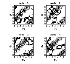
Figure 19: Node activities in layer 3 as a function of the inputs $\phi_{3}$ and $\phi_{4}$ (with $\phi_{1}=\phi_{2}=0$) which has the properties of an invariant encoder.

Figure 18 and Figure 19 show the encoder that occurs in stage 3 of Figure 11. This is an invariant encoder of the type shown in Figure 13a, which corresponds to the connectivity seen in Figure 11c.

The diagrams in this section show how a 3-stage chain of linked SVQs of the type shown in Figure 9 self-organises to process hierarchically correlated phase data. Stage 1 makes an approximate copy of the data where each phase is separately encoded, then stage 2 encodes the output of stage 1 discarding the smallest degrees of freedom, and finally stage 3 encodes the output of stage 2 discarding the next smallest degree of freedom. The chain of SVQs has thus split itself into a hierarchical network of linked encoders that is optimally matched to the task of mapping from the original data at the input to the chain to the compressed representation at the output of the chain. This is true self-organisation of multiple encoders unlike the hard-wiring of encoders that is used in other approaches (e.g. [6]).

5 Conclusions

This paper has shown how it is possible to map a data manifold into a simpler form by progressively discarding small degrees of freedom. This is the key to self-organising data fusion, where the raw data is embedded in a very high-dimensional space (e.g. the pixel values of one or more images), and the requirement is to isolate the important degrees of freedom which lie on a low-dimensional manifold. A useful advantage of the approach used in this paper is that it assumes only that the mapping from manifold to manifold is organised in a chain-like topology, and that all the other details of the processing in each stage of the chain are to be learnt by self-organisation. The types of application for which this approach is well-suited are ones in which separation of small and large degrees of freedom is desirable. For instance, separation of targets (small) and jammers (large) is relatively straightforward using this approach [10].

Data that is not embedded in a higher-dimensional space is usually not suitable for processing with the approach used in this paper. For instance, categorical (or symbolic) data that has one of only a few possible states is not suitable, but a smoothly variable array of pixel values is suitable. This type of network is intended to operate on raw sensor data rather than pre-processed data, and typically will use high-dimensional intermediate representations in its processing chain. Because of its ability to compress the raw data into a much simpler form, this type of network would typically be used as a bridge between the sub-symbolic raw sensor data and the symbolic higher level representation of that data.

Although the full connectivity between adjacent layers of the chain implies that the computations can be expensive, after some initial training the factorial structure of the various encoders becomes clear and can be used to prune the connections to keep only the ones that are actually used (i.e. usually only a small proportion of the total number). When the chain is fully trained each code index typically depends on only a small number of contributing inputs (i.e. a receptive field) from the previous stage of the chain. Furthermore, because of the normalisation used in each layer, the size and shape of the receptive fields mutually interact (i.e. there is a fixed total amount of activity in each layer), so the raw receptive fields (i.e. as defined by the feed-forward network weights) are different from the renormalised receptive fields (i.e. after taking account of normalisation).

The network described in this paper passes information along the processing chain in a deterministic fashion, because it uses (hypothetical) histograms containing an infinite number of samples, which thus do not randomly fluctuate. This was done for computational convenience (i.e. to avoid Monte Carlo simulations) and is not a fundamental limitation of the approach used. With additional computational effort it is possible to operate the network as a (non-deterministic) Markov chain in which the histograms contain only a finite number of samples, which therefore randomly fluctuate and explore network states in the vicinity of the deterministic state used in this paper.

6 Acknowledgements

The research presented in this paper was supported by the United Kingdom’s MoD Corporate Research Programme.

References

- [1] Kohonen, T. (2001). Self-Organising Maps. Springer Series in Information Sciences, Vol. 30, Springer-Verlag.
- [2] Martinez, T. M., & Schulten, K. J. (1991). A "neural-gas” network learns topologies. In T. Kohonen, K. Mäkisara, O. Simula & J. Kangas (Ed.), Artificial Neural Networks (pp. 397–402). North-Holland.
- [3] Dittenbach, M., Merkl, D., & Rauber, A. (2000). The growing hierarchical self-organising map. In S. Amari, C. L. Giles, M. Gori & V. Piuri (Ed.), Proceedings of the International Joint Conference on Neural Networks (IJCNN 2000) (pp. 15–19). IEEE Computer Society.
- [4] Luttrell, S. P. (1994). A Bayesian analysis of self-organising maps. Neural Computation, 6(5), 767–794.
- [5] Luttrell, S. P. (2003). A Markov chain approach to multiple classifier fusion. In T. Windeatt & F. Roli (Ed.), Proceedings of the 4th International Workshop on Multiple Classifier Systems (pp. 217–226). Lecture Notes in Computer Science, Vol. 2709, Springer-Verlag.
- [6] Ross, D. A., & Zemel, R. S. (2003). Multiple-cause vector quantisation. In S. Becker, S. Thrun & K. Obermayer (Ed.), Advances in neural information processing systems 15. MIT Press.
- [7] Linde, Y., Buzo, A., & Gray, R. M. (1980). An algorithm for vector quantiser design. IEEE Transactions on Communications, 28(1), 84–95.
- [8] Luttrell, S. P. (1999). Self-organised modular neural networks for encoding data. In A. J. Sharkey (Ed.), Combining Artificial Neural Nets: Ensemble and Modular Multi-Net Systems (Perspectives in Neural Computing) (pp. 235–263). Springer-Verlag.
- [9] Luttrell, S. P. (1997). A theory of self-organising neural networks. In S. W. Ellacott, J. C. Mason & I. J. Anderson (Ed.), Mathematics of Neural Networks: Models, Algorithms and Applications (pp. 240–244). Operations Research/Computer Science Interfaces, Vol. 8, Kluwer.
- [10] Luttrell, S. P. (2002). Using stochastic vector quantisers to characterise signal and noise subspaces. In J. G. McWhirter & I. K. Proudler (Ed.), Mathematics in Signal Processing V (pp. 193–204). OUP.