Parallel Mixed Bayesian Optimization Algorithm: A Scaleup Analysis

Abstract

Estimation of Distribution Algorithms have been proposed as a new paradigm for evolutionary optimization. This paper focuses on the parallelization of Estimation of Distribution Algorithms. More specifically, the paper discusses how to predict performance of parallel Mixed Bayesian Optimization Algorithm (MBOA) that is based on parallel construction of Bayesian networks with decision trees. We determine the time complexity of parallel Mixed Bayesian Optimization Algorithm and compare this complexity with experimental results obtained by solving the spin glass optimization problem. The empirical results fit well the theoretical time complexity, so the scalability and efficiency of parallel Mixed Bayesian Optimization Algorithm for unknown instances of spin glass benchmarks can be predicted. Furthermore, we derive the guidelines that can be used to design effective parallel Estimation of Distribution Algorithms with the speedup proportional to the number of variables in the problem.

1 Introduction

Estimation of distribution algorithms (EDAs) [1, 2] , also called probabilistic model-building algorithms (PMBGAs) [3] and iterated density estimation evolutionary algorithms (IDEAs) [4], are stochastic techniques that combine genetic and evolutionary algorithms, machine learning, and statistics. EDAs are able to effectively discover and mix the building blocks of partial solutions, provided that the allowed complexity of probabilistic model is relevant to optimized problem. In contrast to genetic algorithms, their performance is not affected by the ordering of parameters. The relations between parameters of solved problem are discovered by machine-learning methods and incorporated into the constructed probabilistic model.

The necessary condition of successful EDA is the generality of its probabilistic model. The well known Bayesian Optimization Algorithm (BOA) [5] uses a very general probabilistic model - a Bayesian network - to encode the relations between discrete parameters of the solved problem. Local probability distributions in the Bayesian network in the original BOA were stored using full conditional probability tables. More efficient representation of the local distributions was used in the hierarchical Bayesian Optimization Algorithm (hBOA) [6], which uses decision trees or graphs to represent these local distributions.

The Mixed Bayesian Optimization Algorithm (MBOA) [7] is able to deal with discrete and continuous parameters simultaneously by using a Gaussian kernel model to capture local distributions of continuous parameters. Its detailed principles are described in [8]. In binary domain it can be seen as a variant of hBOA, but its implementation emphasizes the possibility to efficiently perform model building in parallel. The implementation of parallel MBOA was first simulated in the TRANSIM tool [9] and its real implementation was reported in [10].

This paper analyzes the time complexity of parallel Mixed Bayesian Optimization Algorithm for binary domain and compares this complexity with experimental results obtained by solving spin glass optimization problem. The following Section defines the spin glass benchmark and motivates for its parallel solving. Section 3 introduces the main principles of MBOA, and Section 4 analyzes the time complexity of each MBOA part. Section 5 provides the scalability analysis of parallel MBOA, identifies the main parts that have to be performed in parallel and derives the guidelines that can be used to design effective parallel MBOA. The experimental results are presented in Section 6 and conclusions are provided in Section 7.

Note that this paper does not investigate the relation between problem size $n$ and the minimal population size required for its solving $N$, but it provides methods for predicting algorithmic efficiency of parallel MBOA given the problem-dependent relation between $n$ and $N$. See [11] for the analysis of population sizing in BOA.

2 Spin glass benchmark

Finding the lowest energy configuration of a spin glass system is an important task in modern quantum physics. Each configuration of spin glass system is defined by the set of spins

$$S=\{s_{i}|\forall i\in\{1,\ldots,s^{d}\}:s_{i}\in\{+1,-1\}\},$$ (1)

where $d$ is the dimension of spin glass grid and $s$ is the size of spin glass grid. For the optimization by BOA the size of spin glass problem $s^{d}$ is equal to the length $n$ of a solution, thus

$$n=s^{d}$$ (2)

Each spin glass benchmark instance is defined by the set of interactions $\{J_{i,j}\}$ between neighboring spins $s_{i}$ and $s_{j}$ in the grid.

The energy of the given spin glass configuration $S$ can be computed as

$$E(S)=\sum\limits_{i,j\in\{1,\ldots,n\}}{J_{i,j}s_{i}s_{j}}$$ (3)

where the sum runs over all neighboring positions $i$ and $j$ in the grid. For general spin glass systems the interaction is a continuous value $J_{i,j}\in<-1,+1>$, but we focus only on Ising model with either ferromagnetic bond $J_{i,j}=-1$ or antiferromagnetic bond $J_{i,j}=+1$, thus $J_{i,j}\in\{-1,+1\}$. Obviously, in the case of ferromagnetic bond the lower (negative) contribution to the total energy is achieved if both spin are oriented in the same direction, whereas in the case of antiferromagnetic bond the lower (negative) contribution to the total energy is achieved if both spins are oriented in opposite directions. Periodic boundary conditions are used to approximate the properties of arbitrary sized spin glass systems.

3 Mixed Bayesian Optimization Algorithm

3.1 Main principles

The general procedure of EDA algorithm is similar to that of GA, but the classical recombination operators are replaced by learning and sampling a probabilistic model. First, the initial population of EDA is generated randomly. In each generation, promising solutions are selected from the current population of N candidate solutions and the true probability distribution of these selected solutions is estimated. New candidate solutions are generated by sampling the estimated probability distribution. The new solutions are then incorporated into the original population, replacing some of the old solutions or all of them. The process is repeated until the termination criteria are met.

Various models can be used in EDAs to express the underlying probability distribution. One of the most general models is the Bayesian network. A Bayesian network consists of two components. The first is a directed acyclic graph (DAG) in which each vertex corresponds to different variable of optimized problem which is treated as random variable. This graph describes conditional independence properties of the represented distribution. It captures the structure of the optimized problem. The second component is a collection of conditional probability distributions (CPDs) that describe the conditional probability of each variable $X_{i}$ given its parents ${{\Pi}}_{i}$ (ancestors) in the graph. Together, these two components represent an unique probability distribution

$$p(X_{0},...,X_{n-1})=\prod\limits_{i=0}^{n-1}{p(X_{i}|}{{\Pi}}_{i}).$$ (4)

The well known EDA instances with Bayesian network are the Bayesian Optimization Algorithm (BOA)[5] , the Estimation of Bayesian Network Algorithm (EBNA) [12] and the Learning Factorized Distribution Algorithm (LFDA) [13] . All these algorithms use metrics-driven greedy algorithm for construction of dependency graph. The implementation details of Bayesian network construction can be found in [14].

3.2 Advantages of decision trees

The Mixed Bayesian Optimization Algorithm (MBOA) [7] is based on BOA with Bayesian networks, but it uses more effective structure for representing conditional probability distributions in the form of decision trees, as proposed in [6]. It would be unreasonable to parallelize MBOA if we had no evidence about its merits over BOA, because BOA was already parallelized in several variants like PBOA and DBOA [15].

There are several reasons for using decision trees. Firstly, only the coefficients for those combinations of ${\Pi}_{i}$ that significantly affect $X_{i}$ are estimated. With less coefficients the value of each coefficient is – on average – estimated more precisely. Secondly, the model building procedure allows for more precise model, since it explores networks that would have incurred an exponential penalty (in terms of the number of parameters required) and thus would have not been taken into consideration otherwise.

MBOA can be also formulated for continuous domains, where it tries to find the partitioning of a search space into subspaces where the parameters seem to be mutually independent. This decomposition is captured globally by the Bayesian network model with decision trees and the Gaussian kernel distribution is used locally to approximate the values in each resulting partition. Without the loss of generality, in following Sections we will focus on the performance of MBOA in binary domain.

4 Complexity analysis

4.1 Complexity of selection operator

The most commonly used selection operator in EDAs is tournament selection, where pairs of randomly chosen individuals compete to take place in the parent population that serves for model learning. The number of tournaments is $O(N)$ and for each tournament we perform $O(n)$ steps to copy the whole chromozome, so the total complexity is $O(nN)$. This also holds for many other selection operators.

4.2 Complexity of model construction

The sequential hBOA builds all the decision trees at once. It starts with empty trees and it subsequently adds decision nodes. The quality of potential decision nodes is determined by Bayesian-Dirichlet metrics [14] which is able to determine the significance of statistical correlations between combinations of alleles in the population. A necessary condition for adding new split node is the acyclicity of dependency graph - it must be guaranteed that no variables $X_{i}$, $X_{j}$ exist such that $X_{i}$ is used as a split in the tree for gene $X_{j}$ and at the same time $X_{j}$ is used as a split in the tree for gene $X_{i}$. In parallel MBOA it is necessary to build each decision tree separately in different processor, so we need an additional mechanism to guarantee the acyclicity.

In [9, 10] we proposed the method that solves this problem. Each generation it uses random permutation ${\bf o}=(o_{0},o_{1},,o_{n-1})$ to predetermine topological ordering of genes in advance. This means that only the genes can serve as splits in the binary decision tree of target gene. The model causality might be violated by this constraint, but from the empirical point of view the quality of generated models is the same as in the sequential case. The advantage is that each processor can create the whole decision tree asynchronously and independently of the other processors. Consequently, the linear speedup is achieved by removing this communication overhead.

Function BuildTree(Population Pop, TargetVariable Xi,
             ListOfCandidateSplitVariables Pa): DecisionTreeNode;
Begin
  Initiate the frequency tables;                          ... O(n)
  For each Variable Xj in Pa                              ... O(n)
    Evaluate the metrics gain of Xj split for Xi target;  ... O(N)
  End for
  Pick up the split Xj’ with the highest quality;         ... O(n)
  Pop1 := SelectIndividuals (Pop,"Xj’ = 0");              ... O(N)
  Pop2 := SelectIndividuals (Pop,"Xj’ = 1");              ... O(N)
  return new SplitNode(new SplitCondition("Xj’"),
                       BuildTree(Pop1,Xi,Pa-{Xj’}),
                       BuildTree(Pop2,Xi,Pa-{Xj’}));
End;

To express the time complexity of whole model building algorithm, we start with the complexity of one run of BuildTree() procedure, which is $O(n+nN+n+N+N)=O(n)+O(nN)$. The total number of BuildTree() calls is $O(2^{h})$, where $h$ is the average height of final decision tree, but note that the population size N is decreased exponentially in the recursion:

$$\sum\limits_{i=1}^{h}{2^{h}.(O(n)+O(nN/2^{h})})\approx\sum\limits_{i=1}^{h}{2^{h}.O(nN/2^{h})}=\sum\limits_{i=1}^{h}{O(nN)}=O(hnN)$$ (5)

To be precise, the time spent on initialization of frequency tables and the time spent on picking-up of the best split is not compensated by this exponential decrease of population size, since it does not depend on $N$. However, in practical cases we can neglect this term because due to the model penalty the depth of recursion stops at some boundary where the population size is still reasonable such that the time required for computation of metrics is always higher than the time for initialization of frequency tables and for picking of the highest gain. The final complexity of building of whole decision tree is thus $O(hnN)$ and the complexity of building whole probabilistic model composed of $n$ decision trees is $O(hn^{2}N)$. On various suites of optimization problems we observed that the depth of decision trees is proportional to $\log(N)$. Hence, the time complexity of model building can be rewritten as $O(n^{2}N\log(N))$. This time complexity also holds for hBOA, but its model building algorithm is not intended for parallel processing.

4.3 Complexity of model sampling

Model sampling generates $O(N)$ individuals of length $n$, where each gene is generated by traversing down the decision tree to the leaf. On average, it takes $O(h)=O(\log(N))$ decisions before the leaf is reached. Thus, the overall complexity of model sampling is $O(nN\log(N))$.

4.4 Complexity of replacement operator

For the MBOA algorithm we use the Restricted Tournament Replacement (RTR) to replace a part of target population by generated offspring. RTR was proposed in [6] and its code can be specified as follows:

For each offspring individual from offspring population   ...O(N)
  For a*N randomly chosen individuals from target pop.  ...O(a*N)
    Compute the distance between chosen individual
            and offspring individual;                     ...O(n)
  End for
  If fitness of offspring individual is higher than the fitness
           of chosen individual with closest distance then
    Replace the chosen individual by offspring individual;...O(n)
  End if
End for

The whole time complexity is then $O(N(anN+n))=O(anN^{2})$, where the coefficient $a$ determines the percentage of randomly chosen individuals in target population that undergo the similarity comparison with each offspring individual. The greater the $a$, the the stronger the pressure on diversity preservation. Note that the complexity of RTR exhibits the complexity of most other existing replacement operators.

4.5 Complexity of fitness evaluation

In the experimental part of this paper we use the spin glass benchmark (defined in Section 2) as a real-world example of an NP complete optimization problem. The evaluation time of one spin glass configuration is linearly proportional to the number of bonds, which is linearly proportional to the number of spins $O(n)$. For $N$ individuals the evaluation time grows with $O(nN)$. This complexity also holds for decomposable deceptive functions and many artificial benchmarks.

Optionally, MBOA can use hill-climbing heuristics to improve the fitness of each individual. This heuristics tries to flip each bit and the change with the highest fitness increase is picked and accepted. This improvement is repeated until no flipping with positive outcome exists. Empirically the number of successful acceptances per chromozome is $O(\sqrt{n})$ and after each acceptance it takes $O(1)$ time to re-compute the outcomes of neighboring flips and $O(n)$ time to pick the best flip for next change. The total complexity of hill climbing heuristics for the whole population is thus $O(nN\sqrt{n})$. The algorithm for picking the best flip for next change can be implemented even more effectively, so the total complexity $O(\log(n)Nn)$ can be achieved. In our analysis we consider the case without heuristics, but we see that the complexity of heuristics only slightly prevails the complexity of spin glass evaluation without heuristics.

5 Scalability analysis

The whole execution time of one generation of MBOA algorithm can be formed by summing up the complexity of selection (weighted by $c_{1}$), model building (weighted by $c_{2}$), model sampling (weighted by $c_{3}$), replacement (weighted by $c_{4}$), and fitness evaluation (weighted by $c_{5}$):

$$c_{1}O(nN)+c_{2}O(n^{2}N\log(N))+c_{3}O(nN\log(N))+c_{4}O(anN^{2})+c_{5}O(nN)$$ (6)

To develop scalable and efficient parallel Mixed Bayesian Optimization Algorithm we need to identify the main tasks that are candidates for parallelization.

Apparently, the most complex part of sequential MBOA is the construction of probabilistic model. Also our experience with solving spin glass benchmarks confirms this statement - typically nearly 95% of the execution time is spent on construction of probabilistic model. In Section 4.2 we outlined an algorithm for parallel construction of Bayesian network with decision trees proposed in [9, 10]. It uses the principle of restricted ordering of nodes in graphical probabilistic model. This method reduces the communication between processors, so the speedup is almost linear and the model building is able to effectively utilize up to $P=n/2$ processors.

As the first case of our analysis, we consider only this parallelization of probabilistic model construction and keep the other parts sequential.

With $P$ processors the overall time complexity of parallel MBOA is

$$c_{1}O(nN)+\frac{1}{P}c_{2}O(n^{2}N\log(N))+c_{3}O(nN\log(N))+c_{4}O(anN^{2})+c_{5}O(nN)$$ (7)

Now we will analyze the proportion between sequential and parallel part of MBOA:

$$\frac{{c_{1}O(nN)+c_{3}O(nN\log(N))+c_{4}O(anN^{2})+c_{5}O(nN)}}{{\frac{1}{P}c_{2}O(n^{2}N\log(N))}}$$ (8)

To obtain an algorithm that is efficiently scalable, this proportion should approach zero as $n$ grows.

5.1 Scalability for fixed number of processors

We first analyze scalability in the case of constant $P$ and increasing $n$. This is the typical scenario when the computational resources are fixed but the problem to be solved is very large. The detailed analysis of terms in fraction (8) for $P=const.$, $n\to\infty$ gives us the following suggestions for design of parallel MBOA:

• The terms with $c_{1}$ and $c_{5}$ are negligible for scalability:

  $$\mathop{\lim}\limits_{n\to\infty}\frac{{c_{1}O(nN)+c_{5}O(nN)}}{{\frac{1}{P}c_{2}O(n^{2}N\log(N))}}=0$$ (9)

  In another words, neither the selection operator nor the population evaluation have to be implemented in parallel. Of course this outcome is valid only for population evaluation with time complexity $O(nN)$. For quadratic complexity of population evaluation $O(n^{2}N)$ the scalability will depend on the absolute values of constants $c_{5}$, $c_{2}$ and on the problem-dependent relation between ”n” and ”N”. Theoretically, if the population size grows linearly with problem size ($N\propto n$) it is still possible to keep the fitness evaluation sequential, because the $\log(N)$ term in the denominator prevails. Nevertheless, in practical situations we suggest parallel evaluation of problems with quadratic and higher complexity. The parallelization of fitness evaluation is solved problem and its implementation is straightforward. For more detailed discussion of parallel fitness evaluation see [16].

• The sampling of model does not have to be performed in parallel, since for all possible assignments to constants $c_{2}$, $c_{3}$ and $P$ it always holds

  $$\mathop{\lim}\limits_{n\to\infty}\frac{{c_{3}O(nN\log(N))}}{{\frac{1}{P}c_{2}O(n^{2}N\log(N))}}=0$$ (10)

• The Restricted tournament replacement has not to be performed in parallel if

  $$\mathop{\lim}\limits_{n\to\infty}\frac{{c_{4}O(anN^{2}))}}{{\frac{1}{P}c_{2}O(n^{2}N\log(N))}}=0$$ (11)

  In this case the scalability highly depends on the problem-dependent relation between $n$ and $N$. Theoretically, even if the population size grows linearly with the problem size ($N\propto n$) the fraction tends to zero because the $\log(N)$ term in the denominator prevails. However, in practical situations we suggest RTR to be performed in parallel.

5.2 Scalability for increasing number of processors

So far we have analyzed the scalability of sequential BOA for fixed number of processors. Now we will analyze how the scalability changes if the number of available processors scales up with $n$. In this case the execution time is reduced by an order of $n$. By assuming $P\propto n$, we obtain from Equation (8):

$$\frac{{c_{1}O(nN)+c_{3}O(nN\log(N))+c_{4}O(anN^{2})+c_{5}O(nN)}}{{c_{2}O(nN\log(N))}}$$ (12)

We see that the selection operator and the simple evaluation of population (terms with constants $c_{1}$ and $c_{5}$) can still be implemented sequentially, but it does not hold for fitness evaluation with quadratic and higher complexity any more. The decision about implementation of model sampling strongly depends on the required speedup. If sequential model sampling is performed, then the speedup is saturated at $c_{2}/c_{3}$. RTR has to be necessarily implemented in parallel, because for fixed $c_{4}$, $c_{2}$, and $a$ the numerator always prevails the denominator.

6 Experimental results

6.1 Fitting complexity coefficients

We performed a series of experiments on the random instances of 2D Ising spin glass benchmarks of size 100, 225, 400, 625, 900 for population sizes $N=500$, $N=1000$, $N=1500$, $N=2000$, $N=4000$, $N=6000$ and $N=8000$. We measured separately the duration of each part of sequential MBOA in order to determine the coefficients $c_{1}$,$c_{2}$,$c_{3}$,$c_{4}$,$c_{5}$. The fitted coefficients are stated in Tab. 1. We observed that for larger problem sizes the fitting is in agreement with the empirical data, but for lower problem sizes the measured time is smaller than that expected from the theoretical complexity. This can be explained by the effects of cache memory.

MBOA part	Coefficient	Estimated value	R-squared value
selection	$c_{1}$	8.73E-09	$0.978$
model building	$c_{2}$	1.00E-07	$0.979$
model sampling	$c_{3}$	1.58E-07	$0.934$
replacement (RTR)	$c_{4}*a$	2.18E-10	$0.989$
evaluation	$c_{5}$	1.34E-07	$0.918$

Table 1: The resulting values of coefficients $c_{1}$,$c_{2}$,$c_{3}$,$c_{4}$,$c_{5}$. For each Ising spin glass size 100, 225, 400, 625, 900 and each population size $N=500$, $N=1000$, $N=1500$, $N=2000$, $N=4000$, $N=6000$, and $N=8000$ we choose 10 random benchmark instances and averaged the duration of each MBOA part. The coefficients hold for one generation of MBOA performed on Intel Pentium-4 at 2.4 GHz. The slopes of linear trend lines were determined in MS Excel.

6.2 Using complexity coefficients

The obtained coefficients can be used to predict the speedup of MBOA with parallel model building. Given the problem size $n$, the population size $N$, and the number of processors $P$, we get:

$$S=\frac{{c_{1}nN+c_{2}n^{2}N\log(N)+c_{3}nN\log(N)+c_{4}anN^{2}+c_{5}nN}}{{c_{1}nN+\frac{1}{P}c_{2}n^{2}N\log(N)+c_{3}nN\log(N)+c_{4}anN^{2}+c_{5}nN}}$$ (13)

Fig. 1 shows how the predicted speedup changes for increasing $P$ and compare it with the speedup computed from the measured duration of each part of sequential MBOA. We considered 3 different sizes of spin glass instances 20x20, 25x25, and 30x30 and we linearly increased the population size with problem size ($N=4000$, $N=6000$, $N=8000$). As one can see, the predicted speedup fits nicely the empirical speedup, namely for large problem size where the caching effects disappear. Also, it can be seen that it is possible to use larger number of processors (more than $P=50$) without observing any significant speedup saturation.

Note that Equation (13) assumes that the model building is ideally parallelized. This is why we were able to calculate the speedup using the time measurements from sequential MBOA. In practical situations the communication time required by master to communicate the population and to gather the parts of the model from slave processors has to be considered as well. In this analysis we neglect this term because the implementation of message passing interface (MPI) might be platform-dependent and its theoretical time complexity is not known. The speedup measured on the implementation of parallel MBOA using Beowulf cluster of 502 Intel Pentium III computational nodes is shown in Fig. 2 obtained from [10].

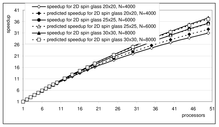
Figure 1: The comparison of the speedup predicted from the numerical fit and the speedup computed from the empirical data measured on sequential BOA solving 2D Ising spin glass instances of size 20x20, 25x25, and 30x30. Population size scales approximately linearly with the problem size.

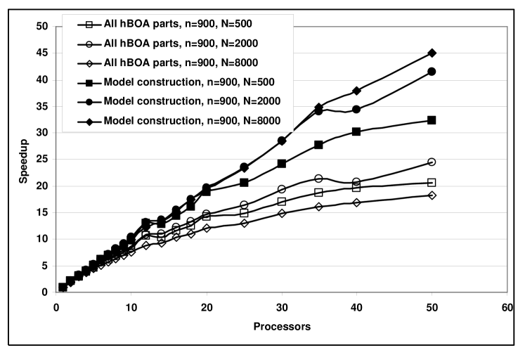
Figure 2: Speedup of the whole parallel MBOA and the speedup of model building part (including true MPI communication) on random spin glass instance with 30x30 spins.

7 Conclusions and future work

We analyzed the time complexity of Mixed Bayesian Optimization Algorithm and fitted this complexity to experimental data obtained by solving spin glass optimization problem. The empirical results fit well the theoretical time complexity equation, so the scalability and algorithmic efficiency of parallel Mixed Bayesian Optimization Algorithm can be predicted, e.g. the speedup for given spin glass size and given number of processors can be determined.

Furthermore, we derive the guidelines that can be used to design effective parallel Estimation of Distribution Algorithms for arbitrary optimization problems where the relation between problem size and the minimal population size required for solving the problem is known. Especially, we focus on the identification of the parts of MBOA which have to be implemented in parallel.

So far the model building was the only part considered to be performed in parallel, but our analysis identified that under some circumstances the parallelization of other parts of MBOA might be required as well. For example, the parallel fitness evaluation (see [16]) can be implemented for problems with expensive fitness evaluation. With careful parallelization of all necessary MBOA parts the achieved speedup is proportional to the problem size. The implementation of all critical MBOA parts in parallel will be a subject of future work.

References

- [1] Mühlenbein, H. and G. Paass: 1996, ‘From Recombination of Genes to the Estimation of Distributions: I. Binary Parameters’. Lecture Notes in Computer Science, 1141, pp. 178–187, 1996.
- [2] Larranaga, P., Lozano, J. A.: Estimation of Distribution Algorithms. A new Tool for Evolutionary Computation. Kluwer Academic Publishers, pp. 57–100, 2002.
- [3] Pelikan, M., Goldberg, D., E., Lobo, F.: A survey of optimization by building and using probabilistic models, IlliGAL Report No. 99018, University of Illinois at Urbana-Champaign, Illinois Genetic Algorithms Laboratory, Urbana, Illinois, 1999.
- [4] Bosman, P. A. N., Thierens, D.: An algorithmic framework for density estimation based evolutionary algorithms. Utrecht University Technical Report UU-CS-1999-46, Utrecht, 1999.
- [5] Pelikan, M., Goldberg, D. E., Cant -Paz, E.: BOA: The Bayesian optimization algorithm. Proceedings of the Genetic and Evolutionary Computation Conference GECCO-99, volume I, Orlando, FL, Morgan Kaufmann Publishers, pp 525–532, 1999.
- [6] Pelikan, M., Goldberg, D., E., Sastry, K.: Bayesian Optimization Algorithm, Decision Graphs, and Occam’s Razor, IlliGAL Report No. 2000020, University of Illinois at Urbana-Champaign, Illinois Genetic Algorithms Laboratory, Urbana, IL, 2000.
- [7] Ocenasek, J., Schwarz, J.: Estimation of Distribution Algorithm for mixed continuous discrete optimization problems, In: 2nd Euro-International Symposium on Computational Intelligence, Kosice, Slovakia, IOS Press, pp. 227–232, 2002.
- [8] Ocenasek, J.: Parallel Estimation of Distribution Algorithms. PhD. Thesis, Faculty of Information Technology, Brno University of Technology, Brno, Czech Rep., pp. 1–154, 2002.
- [9] Ocenasek, J., Schwarz, J., Pelikan, M.: Design of Multithreaded Estimation of Distribution Algorithms. In: Cant -Paz et al. (Eds.): Genetic and Evolutionary Computation Conference - GECCO 2003. Springer Verlag: Berlin, pp. 1247–1258, 2003.
- [10] Ocenasek, J., Pelikan, M.: Parallel spin glass solving in hierarchical Bayesian optimization algorithm. In: Proceedings of the 9th International Conference on Soft Computing, Mendel 2003, Brno University of Technology, Brno, Czech Rep., pp. 120–125, 2003.
- [11] Pelikan, M., Goldberg, D.E., Cant -Paz, E: Bayesian Optimization Algorithm, Population Sizing, and Time to Convergence, In: Cant -Paz et al. (Eds.): Genetic and Evolutionary Computation Conference - GECCO 2000, Las Vegas, Nevada, Springer Verlag: Berlin, pp. 275–282, 2000.
- [12] Etxeberria, R., Larranaga, P.: Global optimization using Bayesian networks. Second Symposium on Artificial Intelligence (CIMAF-99), Habana, Cuba, pp. 332–339, 1999.
- [13] Muhlenbein, H., Mahnig, T.: FDA a scalable evolutionary algorithm for the optimization of additively decomposed functions. Evolutionary Computation, 7(4), pp. 353-376, 1999.
- [14] Heckerman, D., Geiger, D., Chickering, M.: ’Learning Bayesian networks: The combination of knowledge and statistical data’. Technical Report MSR-TR-94-09, Microsoft Research, Redmond, WA, 1994.
- [15] Ocenasek, J., Schwarz, J.: The Distributed Bayesian Optimization Algorithm for combinatorial optimization, EUROGEN 2001 - Evolutionary Methods for Design, Optimisation and Control, Athens, Greece, CIMNE, pp. 115–120, 2001.
- [16] Cantu-Paz, E.: Efficient and Accurate Parallel Genetic Algorithms. Boston, MA: Kluwer Academic Publishers. 2000.