Blind Detection and Compensation of Camera Lens Geometric Distortions

Abstract

This paper presents a blind detection and compensation technique for camera lens geometric distortions. The lens distortion introduces higher-order correlations in the frequency domain and in turn it can be detected using higher-order spectral analysis tools without assuming any specific calibration target. The existing blind lens distortion removal method only considered a single-coefficient radial distortion model. In this paper, two coefficients are considered to model approximately the geometric distortion. All the models considered have analytical closed-form inverse formulae.
Key Words: Radial distortion, Geometric distortion, Lens distortion compensation, Higher order spectral analysis.

I Introduction

Generally, lens detection and compensation is modelled as one step in camera calibration, where the camera calibration is to estimate a set of parameters describing the camera’s imaging process. Using a camera’s pinhole model, the projection from the 3-D space to the image plane can be described by

$$\lambda\left[\matrix{u\cr v\cr 1}\right]=\underbrace{\left[\matrix{\alpha&\gamma&u_{0}\cr 0&\beta&v_{0}\cr 0&0&1}\right]}_{A_{\rm intr}}\left[\matrix{X\cr Y\cr Z}\right]=ZA_{\rm intr}\left[\matrix{X/Z\cr Y/Z\cr 1}\right],$$ (1)

where the matrix $A_{\rm intr}$ denotes the camera’s intrinsic matrix. $(\alpha,\gamma,\beta,u_{0},v_{0})$ are the camera’s five intrinsic parameters, with $(\alpha,\beta)$ being two scalars in the two image axes, $(u_{0},v_{0})$ the coordinates of the principal point (which is also assumed to be at the center of distortion in this paper), and $\gamma$ describing the skewness of the two image axes. In the imaging process described by (1), the effect of lens distortion has not been considered.

In equation (1), $(u,v)$ is not the actually observed image point since virtually all imaging devices introduce certain amount of nonlinear distortions. Among the nonlinear distortions, radial distortion, which is performed along the radial direction from the center of distortion, is the most severe part [1, 2]. In the category of polynomial radial distortion modeling, the commonly used radial distortion function is governed by the following polynomial equation [3, 4, 5, 6, 7, 8]:

$$r_{d}=r+\delta_{r}=r\,f(r,{\bf k})=r\,(1+k_{1}r^{2}+k_{2}r^{4}+k_{3}r^{6}+\cdots),$$ (2)

where ${\bf k}=[k_{1},k_{2},k_{3},\ldots]$ is a vector of distortion coefficients. $r$ and $r_{d}$ can be defined either in the camera frame as [3, 4, 5, 6]

$$r_{\rm xy}=\sqrt{x^{2}+y^{2}},\quad r_{\rm dxy}=\sqrt{x_{d}^{2}+y_{d}^{2}},$$ (3)

with

$$x=\frac{X}{Z},\quad y=\frac{Y}{Z},$$ (4)

or on the image plane as [7, 8]

$$\begin{array}[]{c}r_{\rm uv}=\sqrt{(u-u_{0})^{2}+(v-v_{0})^{2}},\\[5.0pt] r_{\rm duv}=\sqrt{(u_{d}-u_{0})^{2}+(v_{d}-v_{0})^{2}},\end{array}$$ (5)

where the subscript _d denotes the distorted version of the corresponding ideal projections. The subscripts _uv and _xy denote the definitions on the image plane and the camera frame, respectively. The distortion models discussed in this paper are in the Undistorted-Distorted formulation [9], though similar idea can be applied to the Distorted-Undistorted formulation.

Most of the existing camera calibration and lens distortion compensation techniques require either explicit calibration target, whose 2-D or 3-D metric information is available [4], or an environment rich of straight lines [1]. The above mentioned techniques are suitable for situations where the camera is available. For situations where direct access to the imaging device is not available, such as when down loading images from the web, blind lens removal technique has been exploited based on frequency domain criterion [10]. The fundamental analysis is based on the fact that lens distortion introduces higher-order correlations in the frequency domain, where the correlations can be detected via tools from higher-order spectral analysis (HOSA). However, it has been reported that the accuracy of blindly estimated lens distortion is by no means comparable to those based on calibration targets. Due to this reason, this approach can be useful in areas where only qualitative results are required [10].

The paper is organized as follows. Section II starts with an introduction of the blind lens distortion removal technique, which is based on the detection of higher-order correlations in the frequency domain. In Sec. III, we briefly describe two existing polynomial/rational radial distortion approximation functions, along with our recently developed simplified geometric distortion modeling method. Section IV presents detailed lens distortion compensation results using images from both calibrated cameras and some web images. The previously calibrated cameras act as a validation of the blind lens removal technique. Finally, section V concludes the paper.

II Frequency Domain Blind Lens Detection

In this section, higher-order spectral analysis is first reviewed, which provides the fundamental criterion for the blind lens distortion removal technique [10, 11]. The basic approach of the blind lens distortion removal exploits the fact that lens distortion introduces higher-order correlations in the frequency domain, which can be detected using HOSA tools.

II-A Bispectral Analysis

Higher-order correlations introduced by nonlinearities can be estimated by higher-order spectra [11]. For example, third-order correlations can be estimated by bispectrum, which is defined as

$$B(\omega_{1},\omega_{2})=E\{F(\omega_{1})F(\omega_{2})F^{*}(\omega_{1}+\omega_{2})\},$$ (6)

where $E\{\cdot\}$ is the expected value operator and $F(\omega)$ is the Fourier transform of a stochastic one-dimensional signal in the form of

$$F(\omega)=\sum^{\infty}_{k=-\infty}f(k)e^{-j\omega k}.$$ (7)

Notice that the bispectrum of a real signal is complex-valued. Since the estimate of the above bispectrum has the undesired property that its variance at each bi-frequency $(\omega_{1},\omega_{2})$ is dependent of the bi-frequency, a normalized bispectrum, called the bicoherence, is exploited, which is defined to be [10, 11]

$$b^{2}(\omega_{1},\omega_{2})=\frac{|B^{2}(\omega_{1},\omega_{2})|}{E\{|F(\omega_{1})F(\omega_{2})|^{2}\}\,E\{|F(\omega_{1}+\omega_{2})|^{2}\}}.$$ (8)

The above bicoherence can be estimated as

$${\hat{b}}(\omega_{1},\omega_{2})=\frac{\frac{1}{N}\sum_{k}F_{k}(\omega_{1})F_{k}(\omega_{2})F^{*}_{k}(\omega_{1}+\omega_{2})}{\sqrt{\frac{1}{N}\sum_{k}|F_{k}(\omega_{1})F_{k}(\omega_{2})|^{2}\frac{1}{N}\sum_{k}|F_{k}(\omega_{1}+\omega_{2})|^{2}}},$$ (9)

which becomes a real-valued quantity. As a measure of the overall correlations, the following quantity is employed in [10]

$$\frac{1}{N^{2}}\sum^{N/2}_{\omega_{1}=-N/2}\sum^{N/2}_{\omega_{2}=-N/2}{\hat{b}}\left(\frac{2\pi\omega_{1}}{N},\frac{2\pi\omega_{2}}{N}\right),$$ (10)

where $N$ is the dimension of the input one-dimensional signal.

II-B Blind Lens Removal Algorithm

Consider a signal $f_{d}(x)$ that is a distorted version of $f(x)$ according to

$$f_{d}(x)=f(x(1+\kappa x^{2})),$$ (11)

with $\kappa$ controlling the amount of distortion. It has been shown in [10] that correlations introduced by the nonlinearity is proportional to the distortion coefficient $\kappa$, where the quantity (10) is chosen as the measure of the correlations. Now, consider the inverse problem of recovering $f(x)$ from $f_{d}(x)$. It is only when $\kappa$ is properly estimated that the inverted ${\hat{f}}(x)$ contains a least amount of nonlinearities, in which case ${\hat{f}}(x)$ holds a minimum bicoherence.

Based on the above discussions, an intuitive algorithm applied for the blind lens distortion removal is listed in the following [10]:

• Select a range of possible values for the distortion coefficients $\bf\kappa$.

• For each $\bf\kappa$, perform inverse undistortion to $f_{d}(x)$ yielding a provisional undistortion function $f_{\bf\kappa}(x)$.

• Compute the bicoherence of $f_{\bf\kappa}(x)$.

• Select the $\bf\kappa$ that minimizes all the calculated bicoherence of the undistorted signals.

• Remove the distortion using the distortion coefficient obtained from step 4).

III Lens Distortion Modeling

The radial distortion model applied for the blind lens distortion removal in [10] is

$$r_{\rm duv}=r_{\rm uv}(1+k_{\rm uv}\,r^{2}_{\rm uv}),$$ (12)

which is equivalent to

$$\begin{array}[]{c}(u_{d}-u_{0})=(u-u_{0})(1+k_{\rm uv}\,r^{2}_{\rm uv}),\\[5.0pt] (v_{d}-v_{0})=(v-v_{0})(1+k_{\rm uv}\,r^{2}_{\rm uv}),\end{array}$$ (13)

when assuming the center of distortion is at the principal point.

Besides the radial distortion modeling, we have recently proposed a simplified geometric lens distortion modelling method, where lens distortion on the image plane can be modelled by [12]

$$\begin{array}[]{c}(u_{d}-u_{0})=(u-u_{0})\,f(r_{\rm uv},{\bf k}_{\rm uv1}),\\[5.0pt] (v_{d}-v_{0})=(v-v_{0})\,f(r_{\rm uv},{\bf k}_{\rm uv2}),\end{array}$$ (14)

where $f(r_{\rm uv},{\bf k}_{uv1,2})$ can be chosen to be any of the available distortion functions. To illustrate the simplified geometric distortion idea, in this paper, $f(r_{\rm uv},{\bf k}_{uv1})$ and $f(r_{\rm uv},{\bf k}_{uv2})$ are chosen to be the following rational functions [LiliSub2ITMI03Rational]:

$$\begin{array}[]{c}\displaystyle f(r_{\rm uv},k_{\rm uv1})=\frac{1}{1+k_{\rm uv1}r_{\rm uv}^{2}},\\ \displaystyle f(r_{\rm uv},k_{\rm uv2})=\frac{1}{1+k_{\rm uv2}r_{\rm uv}^{2}},\end{array}$$ (15)

for its fewer number of distortion coefficients and the property of having analytical geometric undistortion formulae. From equations (14) and (15), we have

$$(u_{d}-u_{0})^{2}(1+k_{\rm uv1}{\bar{r}}_{\rm uv})^{2}+(v_{d}-v_{0})^{2}(1+k_{\rm uv2}{\bar{r}}_{\rm uv})^{2}={\bar{r}}_{\rm uv},$$ (16)

with ${\bar{r}}_{\rm uv}\stackrel{{\scriptstyle\Delta}}{{=}}r^{2}_{\rm uv}$. The above equation is a quadratic function in ${\bar{r}}_{\rm uv}$, thus having analytical inverse formula.

IV Experimental Results

In this section, we first verify that the blind lens removal technique, which is based on the detection of higher-order correlations in the frequency domain, can be used for the detection and compensation for lens distortion. This verification is via the comparison of the calibration coefficients of the blind removal technique with those calibrated by a planar-target based calibration method [4]. Though, the calibration results by the blind removal technique are by no means comparable to those based on calibration target, the results shown in Sec. IV-A does manifest a reasonable accuracy, at least for applications where only qualitative performance is required.

The existing blind lens distortion removal method only considered a single-coefficient radial distortion model, as described in (12). In Sec. IV-B, we show that cameras, which are more accurately modelled by different distortion coefficients along the two image axes, can also be detected using higher-order correlations. As an example, the simplified geometric distortion modeling with the distortion function (15) is applied. Using single-coefficient to describe the distortion along each image axis, totally two coefficients are used in (15). One reason for choosing the function (15) is in its fewer number of distortion coefficients that reduces the whole optimization duration. Another advantage lies in that equation (15) has analytical geometric inverse formula, which further advances the optimization speed.

Finally, lens distortion compensation of several web images are performed using the blind removal technique.

IV-A Verification of Blind Lens Compensation Using Calibrated Cameras

Comparisons between the distortion coefficients calibrated by the blind removal technique with those obtained by the target-based calibration method have been performed in [10] using distortion function (12). Similar comparison is given here via two calibrated cameras, the desktop [13] and the ODIS camera [14], using the distortion function (12), along with the function (15) with $k_{\rm uv1}=k_{\rm uv2}$. We think that this double verification is needed since lens nonlinearity detection using higher-order spectral analysis is a recent development.

Original images of the desktop and the ODIS cameras are shown in Fig. 1, where the plotted dots in the center of each square are used for judging the correspondence with the world reference points for the target-based calibration. Using the single-coefficient radial distortion model in (15) (with $k_{\rm uv1}=k_{\rm uv2}$), the blindly compensated images of the two cameras are shown in Fig. 2. An image interpolation operator is applied during the lens distortion compensation, since the observed original images are shrinked due to the negative distortion coefficients. The undistorted images are only plotted in gray-level to illustrate the lens compensation results. Comparing Fig. 1 with Fig. 2, it can be observed that lens distortion is reduced significantly, though not completely and perfectly.

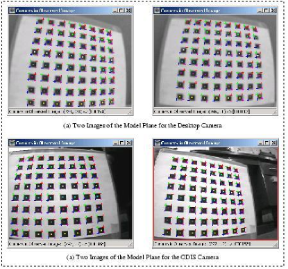
Figure 1: Two Sample images of the model plane with the extracted corners (indicated by cross) for the desktop and ODIS cameras.

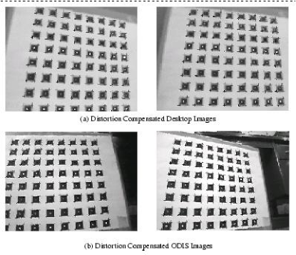
Figure 2: Blindly radially compensated desktop and ODIS images with distortion function (15) with $k_{uv1}=k_{uv2}$.

Using the planar calibration target observed by the cameras as shown in Fig. 1, the desktop and ODIS cameras have been calibrated in [12, LiliSub2ITMI03Rational] using the planar-based camera calibration technique described in [4]. However, the calibrated camera parameters in [12, LiliSub2ITMI03Rational] are in the normalized camera frame, while the blind removal technique deals with distortions in the image plane directly. A transformation between the lens distortion coefficients in the camera frame and those in the image plane is thus needed.

A rough transformation is illustrated in the following using the obtained intrinsic parameters from the planar-target based calibration technique. From equation (1), we have

$$(u-u_{0})=\alpha x+\gamma y,\quad(v-v_{0})=\beta y.$$

Assuming that

$$\gamma\approx 0,\quad\alpha\approx\beta,$$ (17)

for a coarse approximation and using a single-coefficient radial distortion model (12), we have

$$r_{\rm duv}=\alpha\,r_{\rm dxy},\quad r_{\rm uv}=\alpha\,r_{\rm xy}.$$ (18)

The relationship between $k_{\rm uv}$ and $k_{\rm xy}$ can be determined straightforward as

$$k_{\rm uv}=k_{\rm xy}/\alpha^{2}.$$ (19)

In this paper, blind lens distortion compensation is implemented via Matlab using higher-order spectral analysis toolbox following the procedures listed in Sec. II-B. However, instead of using equation (10) as the objective function to minimize, the maximum value of bicoherence is used in our implementation as the measurement criterion for nonlinearity, which is

$$J=\frac{1}{N_{1}N_{2}}{\bf\max}_{\omega_{1}\in[-\frac{N}{2},\frac{N}{2}],\;\omega_{2}\in[-\frac{N}{2},\frac{N}{2}]}{\hat{b}}\left(\frac{2\pi\omega_{1}}{N},\frac{2\pi\omega_{2}}{N}\right),$$ (20)

for an input image of dimension $N_{1}\times N_{2}$.

Comparison of the distortion coefficients obtained from the blind removal and the target-based [4] calibration techniques is shown in Table. I using the functions (12) and (15) with $k_{\rm uv1}=k_{\rm uv2}$. It can be observed from Table I that, despite the deviation of the blindly calibrated results from those based on calibration targets, there is a consistency about the trend qualitatively. Notice that the distortion coefficients under the “Target” column in Table I are obtained via approximations, where of course more precise transformations can be achieved without applying the assumptions in (17). However, since currently the blind removal method considers only the lens distortion (no calibration of the center of distortion), precise comparison can not be achieved even with precise calculation from the side of the target-based algorithm. Generally, the comparison can only be performed “quantitatively”, though the blind removal technique does provide another quantitative criterion for evaluating the calibration accuracy.

TABLE I: Comparison of Lens Distortion Coefficients of the Blind Removal Technique and The Target-Based Algorithm

		Blind Technique ($10^{-6}$)		Target
Eqn.	Camera	Values	Mean	($10^{-6}$)
	Desktop	$-[3.5,4.5,3.5,4.5,1.5]$	-3.5	$-3.73$
(12)	ODIS	$-[3.5,2.5,2.5,3.5,3.5]$	-3.1	$-4.13$
	Desktop	$[5,6,5,5,1]$	4.4	$4.27$
(15)∗	ODIS	$[5,3,4,5,4]$	4.2	$4.75$

${}^{*}k_{uv1}=k_{uv2}$ for modeling the radial distortion.

One issue in the implementation is how to select the searching range for an image. While image normalization method is commonly applied, in our simulation, the searching range is determined based on the image’s dimension and the observed judgement of radial or pincushion distortions in a non-normalized way. This is the reason why in Table I, all the distortion coefficients are very small values. More specifically, consider the radial distortion function (12) with the maximum possible distortion at the image boundary. Let $r=r_{\rm max}$ and $r_{d}=\rho\,r_{\rm max}$, where $r_{\rm max}$ is defined to be $r_{\rm max}=\sqrt{u_{0}^{2}+v_{0}^{2}}$ on the image plane and the subscript _uv is dropped for simplicity. We have

$$k_{\rm uv}=\frac{\rho-1}{r^{2}_{\rm max}}.$$ (21)

For our desktop and ODIS images, the dimension of the images is $320\times 240$ in pixel. Further, the distortion experienced by these two cameras is a barrel distortion with $r_{d}<r$. Focusing on the barrel distortion by considering $\rho\in[0,\frac{1}{4},\frac{1}{2},\frac{3}{4},1]$, we have

$$k_{\rm uv}=\left\{\matrix{-6.25\times 10^{-6},&{\rm when}\;\rho=\frac{3}{4},\cr 0,&{\rm when}\;\rho=1.}\right.$$ (22)

The initial searching range for the distortion coefficients when using the radial distortion function (12) is chosen to be within $[-4.5\times 10^{-6}\sim 3.5\times 10^{-6}]$ with a step size $10^{-6}$. Similarly, for the radial distortion function (15) with $k_{\rm uv1}=k_{\rm uv2}$, we have

$$k_{\rm uv}=\frac{\frac{1}{\rho}-1}{r^{2}_{\rm max}},$$ (23)

and

$$k_{\rm uv}=\left\{\matrix{8.3\times 10^{-6},&{\rm when}\;\rho=\frac{3}{4},\cr 0,&{\rm when}\;\rho=1.}\right.$$ (24)

The initial searching range when using function (15) is $[0\sim 9\times 10^{-6}]$.

Relative values of $J$ as defined in (20) of the five ODIS images using the distortion functions (12) and (15) with $k_{uv1}=k_{uv2}$ are shown in Figs. 3 and 4. The relative $J$ values equal to their corresponding values minus the minimum value in this group.

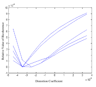
Figure 3: Relative $J$ values of the ODIS images using function (12).

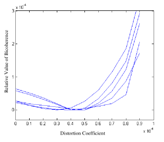
Figure 4: Relative $J$ values of the ODIS images using function (15).

IV-B Blind Detection and Compensation of Lens Geometric Nonlinearity

Besides the radial distortion modelling, a simplified geometric distortion modelling method has been developed in [12]. A straightforward question asked is whether the higher-order correlation detection in the frequency domain can help for the detection of geometric distortions, instead of just the radial one. The above problem is pursued in the next, where we would like to first describe our conclusion. That is, the blind lens removal technique helps to detect the possible geometric distortion of a camera. By allowing the two distortion coefficients along the two image axes searched separately in two regions, the blindly calibrated lens distortion coefficients manifest noticeable difference for cameras that have been reported to be more accurately modelled by a geometric distortion modelling method.

Again using the two calibrated desktop and the ODIS cameras, the blindly calibrated distortion coefficients $k_{\rm uv1}$ and $k_{\rm uv2}$ using the rational distortion function (15) are shown in Table II, where the difference between the two distortion coefficients is significant for the ODIS camera, which has been studied in [12] to be better modelled by a geometric distortion model than a radial one. It is also observed that this difference between distortion coefficients along the two image axes is exaggerated using the blind removal technique.

TABLE II: Blind Detection of Geometric Distortion

	Desktop ($10^{-6}$)	ODIS ($10^{-6}$)
	$[k_{\rm uv1},k_{\rm uv2}]$	$[k_{\rm uv1},k_{\rm uv2}]$
	$[6.16,5.28]$	$[2.64,6.16]$
	$[2.64,4.40]$	$[4.40,6.16]$
Distortion	$[5.28,6.16]$	$[2.64,4.40]$
Coefficients	$[2.64,3.52]$	$[5.28,6.16]$
	$[5.28,3.52]$	$[3.52,6.16]$
Mean	$[4.40,4.57]$	$[3.70,5.81]$

In our implementation, geometric undistortion is implemented using equation (15) for each slice passing through the image center, which is chosen to be 12 degree apart for each image. After $(u,v)$ are derived from $(u_{d},v_{d})$ and $(k_{\rm uv1},k_{\rm uv2})$, where the $(k_{\rm uv1},k_{\rm uv2})$ are determined through the searching procedures, $r_{\rm uv}$ is calculate from $(u,v)$ and the image center (which is assumed to be the center of distortion in the context of blind lens distortion removal technique). Nonlinearity detection using bicoherence is performed on this one-dimensional signal $r_{\rm uv}$, which is basically the same procedures used in the blind removal of radial distortion.

Due to the available knowledge of the distortion coefficients for the two sets of images using the radial distortion modeling with function (15) for $k_{uv1}=k_{uv2}$, when performing the detection for possible geometric distortions, the searching ranges are chosen to be around the distortion coefficients already determined in the radial case.

V Concluding Remarks and Discussions

Higher-order correlation based technique is a promising method to detect lens nonlinearities in the absence of the camera. Besides the commonly used single-coefficient polynomial radial distortion model, blind detection of the geometric distortion is addressed in this paper. Using the quantitative measurement criterion defined in the frequency domain, difference between the two sets of distortion coefficients along the two image axes can be used to detect cameras that are better modelled by a geometric distortion modelling method qualitatively.

References

- [1] Frederic Devernay and Olivier Faugeras, “Straight lines have to be straight,” Machine Vision and Applications, vol. 13, no. 1, pp. 14–24, 2001.
- [2] Roger Y. Tsai, “A versatile camera calibration technique for high-accuracy 3D machine vision metrology using off-the-shelf TV cameras and lenses,” IEEE Journal of Robotics and Automation, vol. 3, no. 4, pp. 323–344, Aug. 1987.
- [3] Chester C Slama, Ed., Manual of Photogrammetry, American Society of Photogrammetry, fourth edition, 1980.
- [4] Zhengyou Zhang, “Flexible camera calibration by viewing a plane from unknown orientation,” IEEE Int. Conf. on Computer Vision, pp. 666–673, Sept. 1999.
- [5] J. Heikkil and O. Silvn, “A four-step camera calibration procedure with implicit image correction,” in IEEE Computer Society Conference on Computer Vision and Pattern Recognition, San Juan, Puerto Rico, 1997, pp. 1106–1112.
- [6] Janne Heikkila and Olli Silven, “Calibration procedure for short focal length off-the-shelf CCD cameras,” in Proceedings of 13th International Conference on Pattern Recognition, Vienna, Austria, 1996, pp. 166–170.
- [7] Charles Lee, Radial Undistortion and Calibration on An Image Array, Ph.D. thesis, MIT, 2000.
- [8] Juyang Weng, Paul Cohen, and Marc Herniou, “Camera calibration with distortion models and accuracy evaluation,” IEEE Trans. on Pattern Analysis and Machine Intelligence, vol. 14, no. 10, pp. 965–980, Oct. 1992.
- [9] Toru Tamaki, Tsuyoshi Yamamura, and Noboru Ohnishi, “Unified approach to image distortion,” in International Conference on Pattern Recognition, Aug. 2002, pp. 584–587.
- [10] Hany. Farid and Alin C. Popescu, “Blind removal of lens distortion,” Journal of the Optical Society of America A, Optics, Image Science, and Vision, vol. 18, no. 9, pp. 2072–2078, Sept. 2001.
- [11] Jerry M. Mendel, “Tutorial on higher-order statistics (spectra) in signal processing and system theory: Theoretical results and some applications,” Proceedings of the IEEE, vol. 79, no. 3, pp. 278–305, Mar. 1991.
- [12] Lili Ma, YangQuan Chen, and Kevin L. Moore, “A family of simplified geometric distortion models for camera calibration,” http:// arxiv.org/ abs/cs.CV/0308003, 2003.
- [13] Lili Ma, “Camera calibration: a USU implementation,” CSOIS Technical Report, ECE Department, Utah State University, http://arXiv.org/abs/cs.CV/0307072, May, 2002.
- [14] “Cm3000-l29 color board camera (ODIS camera) specification sheet,” http ://www. video- surveillance -hidden -spy -cameras.com/ cm3000l29.htm.