Fast Simulation
of Multicomponent Dynamic Systems

Abstract

A computer simulation has to be fast to be helpful, if it is employed to study the behavior of a multicomponent dynamic system. This paper discusses modeling concepts and algorithmic techniques useful for creating such fast simulations. Concrete examples of simulations that range from econometric modeling to communications to material science are used to illustrate these techniques and concepts. The algorithmic and modeling methods discussed include event-driven processing, “anticipating” data structures, and “lazy” evaluation, Poisson dispenser, parallel processing by cautious advancements and by synchronous relaxations. The paper gives examples of how these techniques and models are employed in assessing efficiency of capacity management methods in wireless and wired networks, in studies of magnetization, crystalline structure, and sediment formation in material science, in studies of competition in economics.

1 Introduction

Dynamic systems with many interacting components are encountered in areas ranging from econometric modeling to communications to material science. Individual components and their local interactions may or may not be complex, but their mere multiplicity often creates a complexity which needs to be addressed.

As an example, consider the Flexchan feature, introduced in new releases of the TDMA wireless system. According to the Flexchan method, each base station that serves a cell in the service area, periodically checks interference level on different channels and dynamically rearranges the channels in the order of the increase of the expected interference. A new service request (a new call or a handoff request from a mobile with the call in progress) is allocated according to an accepted strategy taking into account availability of free channels and the segregation order. For instance, a “greedy” strategy places the call on the unoccupied channel with the least expected interference.

All the channel capacity of the system is potentially available to each cell in Flexchan in contrast with Fixed allocation schemes, that are largely in use today. The latter prespecifies a partition of capacity among the cells in anticipation of the traffic. Under the Flexchan, cells themselves negotiate the capacity, dynamically forming an allocation pattern in response to the actual traffic. Thus, the Flexchan eliminates the manual planning, reduces the operating cost and presumably increases capacity and QoS.

Does it? Will the channel segregation adapt to the traffic, or maybe it will instead oscillate somehow, with base stations “fighting” each other for the capacity? If it does adapt, how long would the adaptation process take depending on algorithm parameters such as the frequency of checking the interference by base stations? Short of actual system deployment, only simulations can answer these questions.

To be convincing, the simulation should be dynamic with base stations asynchronously working out their Flexchan routine while users are moving in the service area. Many base stations should be represented in order to demonstrate the algorithm viability; it is possible to imagine how the algorithm would work for just a few base stations, but break down for, say, a hundred base stations. It becomes obvious that a crucial element of this simulation is the computing efficiency of the simulation algorithm.

This paper reviews algorithmic and programming techniques which were used to answer the posed questions by simulation[1]. The program was written so that, say, for about 100 base stations and 1000 active mobiles, simulating one hour of operation requires only several hours of processing on a single PC or workstation.

Similar algorithmic concepts and techniques for improving efficiency of discrete event simulations recur in diverse applications such as:

- an econometric model of telephone companies, like AT&T and MCI, fighting among themselves for the residential telephone market quotas. To attract the customers, the players introduce various payment plans, like “Friends and Family” or “Volume discount.” A question may be: which policy/discount works better given the same cost for the player. The customers behave randomly, their response is staggered, but they tend to behave in accordance with their individual economic interests. It was possible to simulate such systems with more than 100,000 customers with individualized connections and “habits” in calling each other during several simulated years with a single run taking a few minutes on a PC.

- a dynamic routing in a wired network, like the long distance AT&T network, where the use of an “anticipating” data structure allows one to cut processing time of simulating one operating hour from a hundred hours to under a ten hours and where further speed improvement using parallel processing shrinks the processing time to a few minutes.

- multiparticle studies in computational physics, and material science, such as a model of magnetization, a model of particle deposition, a study of impurity-perturbed crystals. Here “lazy” evaluation, Poisson dispensing, and parallel processing lead to several order of magnitude speed improvements. Some simulations previously thought impossible, as they would take years to complete under old techniques, with the new programming techniques move to the category of possible ones, those that can be completed in several hours.

This paper is organized as follows. Sections 2, 3, and 4 present techniques and concepts for simulating multicomponent systems on a uniprocessor. The advantages and difficulties of event-driven processing are discussed in Section 2, the balance between “lazy” and anticipatory methods of evaluation is explained in Section 3, and a general method of event-driven simulation which avoids, and which is faster than the event list method is introduced in Section 4. Sections 5 and 6 present technique for simulating efficiently large multicomponent systems on a multiprocessor. A “cautious” technique which avoids speculative computations is discussed in Section 5. If the latter technique is not feasible, one may resort to the synchronous relaxation method, presented in Section 6. The lessons learned in the course of the practical application of the discussed methods are discussed in Conclusion.

2 Time-driven vs. event-driven simulations

A time-driven description of a dynamic system involves the global clock. The time-driven computer model keeps in memory the global state of the system and modifies the entire state as the global time advances in finite increments. Although time-driven models are intuitive and convenient to think of, one should try to avoid them in simulations because of their computational inefficiency. Converting the model from the time-driven to an event-driven form, whenever such conversion is possible, is a single best improvement to a computer simulation. That is a classical textbook recommendation. In a general case, it is not known, though, how to do the conversion.

2.1 Time-driven one-dimensional billiards

As an example of the conversion, consider simulation of a collection of chaotically colliding billiard balls. Despite its toyish appearance, the “billiards” simulation technically is non-trivial and has serious applications.

For simplicity consider billiards in one dimension. We may imagine a gutter bounded from both ends, which contains $N$ absolutely hard elastic balls of equal mass and size. The width of the gutter is just enough to let the balls move without friction in one dimension. The gutter is placed horizontally which excludes the effect of gravitation on the ball movements. The gutter filled with $N=4$ balls is shown at the bottom of Figure 1 which also presents the initial time-space trajectories of the balls for times $t>0$. The trajectories are indicated by dashed lines, they are initiated at $t=0$ by the shown positions and velocities.

Figure 1: Billiards in one dimension

To simulate the system evolution in a time-driven way, we integrate equations of motion along small time segments of duration $\Delta t$. Thus, starting with time $0$ we advance the state to time $\Delta t$, then to $2\Delta t$, then to $3\Delta t$, and so on.

If a ball experiences no collision during the advancement interval $(t,t+\Delta t)$, then, because there is no friction, we have

$$x(t+\Delta t)=x(t)+v(t)\Delta t,\ \ \ \ v(t+\Delta t)=v(t)$$ (2.1)

where $x(t)$ is the one-dimensional position coordinate and $v(t)$ is the velocity of the ball (center) at time $t$.

At each step the time-driven method monitors distances between components that might come in contact. Ball-ball collisions are detected by monitoring distances $d(i,i+1)$ between centers of balls $i$ and $i+1$. Such a collision occurs during time interval $(t,t+\Delta t)$ if $d(i,i+1)$ becomes smaller that ball diameter $D$ at time $t+\Delta$, while $d(i,i+1)\geq D$ at time $t$. Once detected, the collision is processed by exchanging velocities of the balls at time $t+\Delta t$:

$${v_{i}}^{new}={v_{i+1}}^{old}\ ,\ \ \ \ \ \ {v_{i+1}}^{new}={v_{i}}^{old}$$ (2.2)

It follows, that for a single ball the algorithm detects and processes at most one collision during a $\Delta t$ step. With a large $\Delta t$, the algorithm may fail to represent interdependent collisions that follow over a single $\Delta t$ step. Hence, $\Delta t$ determines the accuracy of the simulation; smaller $\Delta t$ higher the accuracy.

2.2 An application: impurity perturbed crystal

A high accuracy is required in many applications of the billiards simulation, for instance, for generating a pattern of impurity perturbed crystal. A material scientist might be interested to know the geometry of displacements of particles in a crystal formed of identical particles with a tiny fraction of inserted isolated particles of a different kind, the impurity.

Figure 2: Displacement pattern of particles in a hexagonal crystal perturbed by a larger impurity particle in the center. The assembly consists of about 11000 particles. The outlined central square is reproduced in Figure 3

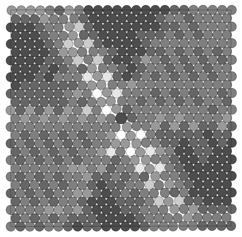
Figure 3: Particle arrangement in the central square oulined in Figure 2. The impurity particle in the center is 20% larger that the rest. Particles have been classified by number of contacts with neighbors according to shading: those that have more contacts with neighbors are darker, white particles are “rattlers” with no contacts

The mechanism of generating a displacement pattern in two dimensions, see Figures 2 and 3, can be modeled by billiards as follow. We introduce an impurity larger particle into a perfect hexagonal crystal of circular particles of common diameter packed inside a bounded geometric shape, say, inside a hexagon. To fit the larger diameter circle we loosen the assembly by simultaneously decreasing the diameters of all the circles. The decrease of the particles matches the excess size of the impurity so that we then able to substitute a single regular particle with the larger impurity particle without creating particle overlaps. The impurity particle is in the center in Figures 2 and 3. We then randomly assign a velocity to each particle and let them all uniformly increase in diameter, so that the ratios of the diameters of the particles remain constant. “Swelling” particles chaotically move in different directions colliding with each other thereby negotiating the limited free space inside the bounded region until the final “jammed” state delivers the sought pattern.

Figure 2 represents vectors of displacement of the particles from their respective original positions in the unperturbed crystal and Figure 3 represents the particles themselves in the central square fragment of the pattern in Figure 2. The pattern is robust. It repeats itself under different initial conditions within a range of parameters such as a ratio of the larger particle to the regular ones and a rate of particle expansion.

At the final phase of the expansion, when the particles are almost “jammed” a quick sequence of interdependent collisions has a high chance to occur within the array of 11,000 particle. The accuracy required for capturing this interdependence is high and the $\Delta t$ required for it is small. Should the $\Delta t$ be not small enough, the simulation fails to produce the correct pattern.

Unfortunately, the accuracy does not agree with the efficiency of computations. In a typical $\Delta t$ step, if the $\Delta t$ is small, the state of most particles is advanced according to (2.1) with no collision. Such is the case for the $\Delta t$ step shown in Figure 1. The no-collision advancements waste computing power: generating the pattern similar to the one shown in Figures 2 and 3 would take more than a year on a personal computer.

That is an estimate though, because the time-driven method was never tried successfully in this example. Instead, the pattern was generated using an event-driven method and the computations for a pattern like the one in Figures 2 and 3 were typically completed in under 10 hours of processing on a PC.

2.3 Event-driven billiards

The event-driven method assumes a discrete event model of the system, wherein the system and its components change their states instantaneously at discrete times; those changes are called the events. The state remains constant on the intervals between the events. The trajectory of the system is a directed acyclic event dependency graph. The nodes of it are the events, and the links represent cause-effect relations in pairs of events.

This graph can be also viewed as a data-flow diagram. To each node-event corresponds the event descriptor, which consists of the time of the event and of the specification of the state change represented by the event. If events $e_{1},e_{2},....,e_{k}$ are all the immediate causes of event $e$, then the descriptor of event $e$ is a function of the descriptors of $e_{1},e_{2},....,e_{k}$. Generating the descriptor of event $e$ from the descriptors of $e$’s causes is processing event $e$.

Figure 1 represents not only the 4-ball system trajectory but can be also viewed as the event dependency graph corresponding to this trajectory. The events $e_{i}$, $i=1,2,...$, are ball-ball and ball-wall collisions. The arrows from an event to an event along a ball trajectory can be seen as cause-effect links on the event dependency graph or as data-dependency links of the data-flow diagram. An event descriptor here consists of: the collision time, the positions and velocities of the involved balls immediately after the collision.

One can check, for instance, that (the descriptor of) event $e_{5}$, a collision of balls 3 and 4, is a function of (the descriptors of) event $e_{4}$, a collision of 2 and 3, and $e_{2}$, a bounce of 4 against the right end of the gutter. Namely, the time component of $e_{5}$ descriptor, $t(e_{5})=t_{5}$, is computed as

$$t_{5}=t_{4}+\frac{x_{4}(t_{2})-x_{3}(t_{4})+v_{4}(t_{2})\ (t_{4}-t_{2})-D}{v_{4}(t_{2})-v_{3}(t_{4})}$$ (2.3)

where $x_{i}(t)$ and $v_{i}(t)$ are position and velocity of ball $i$, $i=1,2,3,4$, at time $t$, $t_{i}=t(e_{i})$ is the time of event $e_{i}$ as indicated on the time axis in Figure 1, and $D$ is the ball diameter. As claimed, the right hand-side in (2.3) is a function of event $e_{2}$ descriptor, including $t_{2}$, $x_{4}(t_{2})$, and (negative) $v_{4}(t_{2})$, and event $e_{4}$ descriptor, including $t_{4}$, $x_{3}(t_{4})$, and (positive) $v_{3}(t_{4})$.

Producing the simulated history of a system under study is the goal of a simulation. The goal is achieved by processing events along the history. But how do we know which events to process? Neither the event descriptors nor the topology of the event dependency graph is known in advance. The event-driven simulation must do both construct the event dependency graph and process the events on it. The former activity, is also referred to as event scheduling.

The task of designing an efficient scheduling usually constitutes the main difficulty of recasting a time-driven model into an event-driven form. A well known mechanism of scheduling an event-driven simulation on a uniprocessor is a queue of events. With the queue one is able to insert future events in the schedule, and to retrieve the next event for processing. A popular data structure [8] for the event queue is heap with which either operation is performed in order of $\text{log}N$ computing operations where $N$ is the number of events in the queue. By contrast, a straightforward scheduling method would need order of $N$ operations either for retrieving or for inserting or for both. If $N=11,000$, say, then slow down may be substantial.

It should be stressed though, that handling event queue efficiently does not cover the entire task of efficient event-driven simulation [15]. The simulationist also has to impose appropriate modeling assumptions. For example, in the simulation of billiards, were the balls not absolutely hard, the collisions would not be instantaneous. Instead of a simple velocity exchange in (2.2), this would force a (slow) time-driven evaluation of the collisions. Equally important for the speed of computation is the assumption of the motion without friction. With friction, the ball motions would not be integrable as simply as in (2.1).

2.4 Mobility of users in wireless simulations

The wireless simulations discussed in Section 1 are naturally of a discrete event type, events being call arrival, termination, handoff, interference measurement, adjustment of the channel segregation order. Among few exceptions is the users’ mobility. The users may move along curvy trajectories with variable speeds. It is decided, however, that the simulated users move with constant velocities along straight line segments. As in the billiards model, this assumption leads to an event-driven processing. Validity of the simulation results is not seriously affected because a curvy motion with variable velocity can be approximated with a sequence of the motions of the considered type.

Selecting a model agreeable with the event-driven mechanism and using an efficient event queue may still be not enough for efficiency of an event-driven simulation. The following sections will discuss more techniques and approaches toward the goal of a fast multicomponent simulation.

3 Anticipatory vs. “lazy” evaluation

A simulation may generate queries concerning the system state. The anticipatory method can be defined as constructing answers for questions which have not yet been asked. It can be contrasted with a “lazy” evaluation method according to which generation of the answer is delayed until the latest possible moment when the query is issued. The anticipatory evaluation tends to be event-driven, while the lazy evaluation time-driven.

3.1 Example: an output statistics

Let us discuss the two approaches in the following simple example. In the wireless simulation, discussed in Section 1, it is necessary to output, as a function of time, the number of mobile users that request but do not obtain a connection. Together with other information, this quantity is to be displayed on the PC screen as the simulation progresses. Thus, given a time increment $\Delta t$, for each time instance $t=0,\Delta t,2\Delta t,\dots$, the simulation is supposed to report the number of $trying$ users among all the users present at time $t$.

The lazy method is straightforward: we scan the list of users and depending on whether a user is $trying$ or non-$trying$ at time $t$, increment the corresponding quantity $trying(t)$ by one or not. Before each scanning instance $t$, we reset counter $trying(t)$ to $0$. This is obviously a time-driven method.

The anticipatory method is driven by events. It does not reset or recompute $trying$ at each reporting time instant. Instead, it maintains the correct value of $trying$ continuously by updating it appropriately at every event which may change $trying$. Such events are: call arrivals to the system, call releases from the system, and users that obtain a connection after a period of retrials. For example, when a user arrives to the system, we would increment $trying$ by one if the user does not immediately get connected.

Note that both solutions “deliver” the same value of counter $trying$. This facilitates the development of the simulation program. In the initial phase, one may program a simpler lazy solution. Then an anticipatory solution should be programmed. Both solutions should then be tried in representative examples, where first we compare values of the results, and then, after the values are found identical, we compare the running times.

3.2 Space sectorization

An example of the anticipatory data structure is space sectorization. Billiards simulation in dimensions two and higher share this method with wireless mobile simulations. The query, in the case of wireless simulations, may be to locate all the mobiles that are close to a given point $(x,y)$ on the plane. Similar queries exist in the billiards simulation. Let us consider the wireless simulation case. There exists a straightforward method to locate all mobiles which are within a given distance $r$ from the point $(x,y)$. In this method, we would find the position $(x_{m},y_{m})$ of each mobile, compute the distance $r_{m}$ from $(x_{m},y_{m})$ to $(x,y)$, and then select those $m$ for which $r_{m}<r$. In practice, $r$ is small and there are just a few such $m$, but to find them we would have to scan all the mobiles.

A structure that helps reduce the computation cost is partitioning the simulation area into smaller sectors. The geometry of a sector may be different, a usual choice is a square. Given such a square $j$, there is a set of all the mobiles $\{m\}_{j}$ that are inside it. Knowing positions of all the mobiles, we can, of course, find the set $\{m\}_{j}$ using a total scan of all mobiles when a query is offered. In the anticipatory method, we maintain the sets $\{m\}_{j}$ continuously independently of queries. This entails updating two such sets each time a mobile crosses a demarcation line between the squares; the crossing becomes an extra event to process.

Having invested in this anticipatory structure, we now find the mobiles $r$-close to a point $(x,y)$ in a different manner. Namely, we first determine the square $j_{0}$ in which $(x,y)$ is located, then scan nearby squares $j$ that intersect with any circle of radius $r$ with center anywhere in $j_{0}$, and then check only the mobiles that belong to sets $\{m\}_{j}$.

3.3 The balance between anticipatory and lazy computations

The same two query evaluation approaches, anticipatory and lazy, can be considered with respect to Web search engines. For many query types, when a search request is submitted on a Web search service, a lazy on line evaluation of the request is non-feasible. Too few users would be willing to wait for the server to scan the World Wide Web. The global scanning is being performed but off line. Mechanical and manual methods are used to create structures which contain answers to various anticipated questions and mechanisms exist to quickly retrieve these answers concentrated at a few data base sites of the search server.

The “economics” of a Web server query evaluation and that in a simulation are different, though. In the former, high computational and manual labor costs are justifiable by the need of short response time. In the latter, an anticipatory method can be only justified if total computing effort when using the method decreases.

With a lazy evaluation, while there may be high cost of retrieving the answer when needed, no resource is spent for anticipating the question. With an anticipatory evaluation, the cost of retrieving the answer may be smaller, but possibly a high investment may be needed for anticipating the question. Anticipatory mechanisms should be advanced only as far as savings on the retrieving end of the balance are higher than spendings on the investing end.

3.4 Example: a circuit switched network

The situation may be illustrated with the following example [3] of simulating a circuit-switched wired network, like the AT&T telephone network. In the model, the network consists of $N$ nodes that represent the switches and $L=N(N-1)/2$ links that connect the nodes. A link consists of a fixed number (possibly zero) of trunks. The model assumes, that if a call is to be carried along some path in the network, then one trunk from each link on the path must be allocated for the exclusive use of the call. The model also assumes that calls are randomly generated between node pairs ($n_{1},n_{2}$) and that a routing policy decides whether to block (reject) such a call or carry it on some path between $n_{1}$ and $n_{2}$. The simulation is used to assess the quality of different routing policies in terms of the blocking produced for given traffic loads.

Consider the Least Busy Alternative (LBA) policy and the Aggregated Least Busy Alternative (ALBA) policy. Both policies allocate a trunk on the link between nodes $n_{1}$ and $n_{2}$ if an idle trunk is available. If not, both offer the call to a two-link path that uses an additional node $\nu$. The intermediate node $\nu$ is called the via. In LBA policy, the overflowing call is offered to the two-link path that has the most idle capacity. Specifically, path $(n_{1},\nu,n_{2})$ is used if $\nu^{*}=\nu$ maximizes

$$\text{min}(idle(n_{1},\nu),idle(\nu,n_{2}))$$ (3.1)

where $idle(x,y)$ is the number of idle trunks currently on link $(x,y)$. If no idle capacity is available - expression (3.1) is zero for all $\nu$ - then the call is blocked.

The ALBA policy is a coarsening of LBA, which is less costly to implement. The overflow calls are offered to a two-link path with a minimum load class. Load classes are defined by a fixed number of prespecified capacity boundaries. For instance, three load classes can be defined with boundaries 0% $=g_{0}<g_{1}<g_{2}<g_{3}=$ 100% , where say $g_{1}=$80% and $g_{2}=$90%. If on a given link the proportion of occupied trunks is $g$, then the link belongs to the load class $i$ with $g_{i-1}\leq g<g_{i}$. Thus, class 1 contains the lightly loaded links, class 2 contains the moderately loaded links, and class 3 contains the heavily loaded links. The load class of a two-link pass is defined to be the smaller of the load classes of the two links. An overflowing call between $n_{1}$ and $n_{2}$ uses a two-link path whose load class is the minimum among all two-link paths between this node pair. If no two-link path has sufficient idle capacity, then the call is blocked.

The query subject to discussion here is finding the via $\nu$ when no idle capacity exists on the direct path $(n_{1},n_{2})$. The “lazy” method operates exactly as the definition says: when the query is issued, it scans all possible vias $\nu$, for each $\nu$ computes the idle capacity (3.1) and chooses the $\nu$ which yields the maximum to (3.1) in the case of LBA policy, or it chooses a via with the minimum of the load class in the case of ALBA policy.

An anticipatory data structure may be suggested for the case of LBA policy which for each node pair ($n_{1},n_{2}$) consists of a list of vias $\nu$ sorted decreasingly according to (3.1). Whenever a least busy via is needed, the first via in the list is chosen which greatly decreases the computations on the retrieving end of the balance. On the investing end of the balance, each time a trunk is allocated or freed on any link $\nu_{1},\nu_{2}$, the $(N-1)(N-2)$ sorted lists for all links ($n_{1},n_{2}$) which can use either $\nu_{1}$ or $\nu_{2}$ as a via have to be updated. As a result, there is no overall saving if anticipatory approach is used for the LBA simulation.

However, for the ALBA simulation, the anticipatory approach yields a significant improvement comparing with the lazy approach. The capacity of a link is usually measured in hundreds if not thousands of trunks while there are typically only a few, say three load classes. Thus, when a link trunk occupancy changes, the link rarely changes its load class. If the load class does not change, no expensive update of sorted class-via lists is needed.

In the ALBA case, both lazy and anticipatory methods were tried. While a useful lazy simulation run of the network took more than 100 hours, the corresponding anticipatory simulation run took 3 to 10 hours on the same uniprocessor.

3.5 Anticipatory and lazy billiards simulations

We now examine event-driven billiards simulations with respect to the topic of anticipatory vs. lazy evaluation. The query concerning a ball location is better accommodated by the anticipatory sectoring as discussed above. Another basic query in the billiards simulation is: which collision has to be processed next? In the anticipatory method of D. Rapaport [14], the data structure, which accommodates the answer, includes for each ball a set of all future events which can not be easily excluded. (Future collisions with distant balls in dimensions two and higher can be excluded using the sectoring method.) The minimum time event in this list is the best candidate event to next occur with the given ball. The minimum time event among all the best candidates is the query answer. This event is to be processed next.

Maintaining such lists is an easy task for the gutter billiards, as there are only two candidates for a collision with any ball $i$, its left neighbor $i-1$ and its right neighbor $i+1$. (The neighbor may be a gutter end for balls 1 and $N$.)

In higher dimensions, the task of maintaining the lists becomes more involved, since many balls can not be excluded beforehand as candidates for future collisions of a ball, even if using the sectoring method. These anticipatory lists may include large and variable number of candidates and they have to be examined and updated for each event processed.

On the positive side, method [14] handles easily the collision preemption which occurs as follows. Suppose the algorithm schedules a collision of two balls, say $A$ and $B$, for some future time $t_{AB}$ and this collision becomes the best candidate event to occur for each ball $A$ and $B$. However, before the processing reaches time $t_{AB}$, a third ball, say $C$, intercepts ball $A$ with a collision scheduled to occur at time $t_{AC}$ so that $t_{AC}<t_{AB}$. Now, of course, the collision of $A$ with $C$ becomes the best candidate for $A$. What should become the new best candidate for ball $B$ ? The answer is ready, anticipated in the list of ball $B$: the previously rated next-best candidate event for ball $B$ is upgraded in status to become the best candidate.

This anticipatory event-driven algorithm can be contrasted with the method [13], which also presents an event-driven, but “lazy” simulation algorithm for billiards. Here only one future event is kept in each individual ball list. Maintaining this structure is easy: when a better candidate emerges, it replaces the old one, which is simply discarded.

However, we should reexamine for the “lazy” method the described above collision preemption situation with balls $A$,$B$, and $C$. What will be the new candidate event for ball $B$ ? The solution [13] introduces a new event type on a ball trajectory, an “advancement” event. When processing such an event, the ball is advanced to the new position without changing its velocity. Thus, when the collision between $A$ and $B$, which was scheduled for time $t_{AB}$, is preempted by an earlier collision between $A$ and $C$, the new candidate event for ball $B$ is such an advancement to the former collision site with ball $A$. The time of the advancement event is $t_{AB}$, which is the time of the previously scheduled and then discarded collision of $A$ and $B$. This is similar to the time-driven $\Delta t$ advancement in (2.1); the lazy method [13] can be viewed as a fall back to a time-driven mechanism. However, the lazy method proved to be not slower than the anticipatory method, while the overall algorithm is simpler.

4 Poisson dispenser

4.1 A model of telephone providers competition

Consider in more detail mentioned in Section 1 econometric model [10] of two competing telephone providers, name them company 1 and company 2 (the model generalizes easily to $M>2$ providers). The model also includes $N$ telephone customers. At any time instant $t$ each customer subscribes either to company 1 or to company 2. Let $s_{i}(t)$ denote the subscription status of customer $i$, $i=1,...N$, at time $t$, so $s_{i}(t)=1$ or $s_{i}(t)=2$. Potential bill amounts $B_{ki}=B_{ki}(t)$ can be computed for each customer $i$ if being a subscriber to company $k$, $k=1,2$. That is, the service would cost $B_{ki}$ dollars per month to customer $i$ if $s_{i}=k$.

For example, to compute $B_{ki}$ under the MCI’s “Friends and Family” plan, we add up the minutes-per-month customer $i$ calls all his/her calling parties who subscribe to the same provider (here the MCI), and multiply this by the plan discount price. Then we add the minutes-per-month customer $i$ calls the calling parties who subscribe to the other provider, multiplied by the larger regular price.

According to this model, a tendency to switch the provider originates in comparing alternative bills: if $B_{1i}<B_{2i}$ then customer $i$ wants to be served by provider 1, and if $B_{1i}>B_{2i}$, then by provider 2. A customer who subscribes to one provider but wants to be served by the other one is subject to a “pull” to the opposite provider. The intensity of the pull toward provider 1 for customer $i$ who is currently with provider 2 in case $B_{1i}<B_{2i}$ is expressed by the rate $r_{i}=f(B_{2i}-B_{1i})$ where $f()$ is an explicitly defined monotonically increasing function. If such customer $i$ is with provider 2 at time $t$, then during a small time interval $(t,t+\Delta t)$, customer $i$ tosses a coin and switches to provider 1 with probability $r_{i}\Delta t$. If the switch attempt is not successful, the switch is similarly reattempted during the next interval $(t+\Delta t,t+2\Delta t)$, then next interval and so on. A similarly defined “pull” toward company 2 affects a customer $i$ who is currently served by but is not happy with company 1. The switch attempts are statistically independent of each other for different customers within the same $\Delta t$ interval and they do not depend on the system state before time $t$.

The model assumes an individual calling pattern for each customer $i$; the pattern is defined by specifying minutes-per-month $v_{ij}$ customer $i$ calls each “friend” $j$ of his/her. The calling habits of the customers are stationary, that is, the calling volume matrix $\{v_{ij}|1\leq i,j\leq N\}$ is independent of time. The parameters of the providers’ plans, e.g., prices, are also time-independent. (These assumptions can be relaxed.) Despite the stationarity, $B_{ki}$ and the strength $r_{i}$ of the pull may change with time, $B_{ki}~{}=~{}B_{ki}(t)$, $r_{i}~{}=~{}r_{i}(t)$. This is so, because in plans like “Friends and Family” when your call-destination “friend” switches the allegiance, it affects your bill. You become more susceptible to switching to the same provider if your “friend” has done so, and that is what plans like “Friends and Family” count upon.

4.2 Methods of simulating telephone providers competition

An obvious method of simulating the outlined model is time-driven, it proceeds exactly as the model states. Time is increased in small $\Delta t$ steps. At each step each customer who is not satisfied with the provider randomly attempts to switch. Then based on the new assignments $s_{i}$, new $B_{ki}$ and new rates $r_{i}$ are computed to be valid for the next $\Delta t$ step.

Now we describe an alternative event-driven method of simulating this model. The method is based on the observation that the sequence of times of switching allegiance for each customer forms a Poisson process with the rate $r_{i}$ which varies in time, $r_{i}=r_{i}(t)$. Note that a stationary Poisson process (that with a constant arrival rate $r=\text{const}$) can be simulated as a sequence of arrival times $t_{0}<t_{1}<t_{2}...$ with independent distributed exponentially with mean $1/r$ interarrival times. That is, given arrival $t_{m}$, to sample $t_{m+1}$ one draws an independent sample $q$ of a random value uniformly distributed in $0<q<1$, and then one computes $t_{m+1}=t_{m}-\frac{\text{log}_{e}(q)}{r}$.

The Poisson property is preserved when several arrival processes are aggregated into a single arrival process. Say, we have $N$ Poisson arrival processes and $i$th process has arrival rate $r_{i}(t)$, $i=1,...N$. The aggregate process is defined as the one that has an arrival when any component process does. So defined, the aggregate is also a Poisson process. The arrival rate of the aggregate is $R(t)=\sum_{i=1}^{N}r_{i}(t)$.

One way of arranging an event-driven simulation of the competition between the telephone providers is as follows. A next anticipated switch event is associated with each of the $N$ customers. The event time is generated by sampling the exponential distribution with the current rate of “pull” discussed above. The case of rate 0 is reserved for customers who are satisfied with the provider. Such a customer does not wish to switch and the next switch time is set to infinity. The event queue is arranged as usual. Processing each customer switch modifies some rates $r_{i}$. This, in turn, modifies the time remaining to switch in the events scheduled for the affected customers; sometimes it may reduce the rate to 0 which would postpone the switch event to the infinite future.

Having the Poisson property preserved under the aggregation, the event-driven simulation of this model can be arranged in a different way without presampling and then updating future switch events and without the event queue. In the alternative method, these are replaced with the following Poisson dispenser mechanism. A single Poisson arrival stream with rate $R(t)$ is generated and then is being “dispensed” among the component Poisson streams in accordance with their partial arrival rates $r_{i}(t)$, larger the $r_{i}(t)$ more probable is to delegate an arrival of the aggregate process to customer $i$’s process.

Rate $r_{i}(t)$ of a component Poisson process may experience changes within the time interval between the consecutive arrivals of the component process. By contrast, the aggregate rate $R(t)$ remains constant between arrivals of its process. Hence the interarrivals of the aggregate are distributed exponentially; once next event is scheduled its time never gets changed or postponed. This simplifies and speeds up the computing. The dispenser procedure consists of the cyclic repetition of the two steps specified below; the execution begins with $m=1$ and current time $t_{1}=0$.

DO 1. Using the current aggregate arrival rate $R(t_{m})=\sum_{i=1}^{N}r_{i}(t_{m})$,
sample the time increment $\Delta t_{m}$ from the current time $t_{m}$
to the next arrival of the aggregate process. 2. Select a component process $i$ with probability $p_{i}=r_{i}(t_{m})/R(t_{m})$. Advance the current time to $t_{m+1}=t_{m}+\Delta t_{m}$ and change the state of component $i$. Set new arrival rate $r_{i}$ for component $i$ and compute new arrival rates $r_{j}(t_{m+1})$ for components $j$ whose event arrival rates may change as a result of the state change of component $i$. UNTIL the simulation is complete


This procedure is formulated above for a general multicomponent system. In the considered example, a telephone customer is a component, and the state change of component $i$ is switch $s_{i}(t_{m+1})=3-s_{i}(t_{m})$ of the telephone provider for customer $i$, where map $x\leftarrow 3-x$ turns 1 into 2 and 2 into 1 as required to effect the provider switch. Since after the switch the customer is “happy” with the new provider, the new arrival rate in Step 2 is zero; it may become positive again later as a result of “friends” switching. Also, values $p_{i}$, are indeed a probability distribution, as $p_{i}\geq 0$ and $\sum_{i=1}^{N}p_{i}=1$.

In a straightforward method the selection in step 2 is implemented as follows. First, we draw an independent sample $q$ of a random value uniformly distributed in $0<q<1$. Then we scan monotonically non-decreasing sequence $V_{0}=0$, $V_{1}=r_{1}(t_{m})$,… $V_{i}=\sum_{j=1}^{i}r_{j}(t_{m})$,… $V_{N}=\sum_{j=1}^{N}r_{j}(t_{m})$, fitting value $Rq$ between consecutive terms $V_{i-1}\leq Rq<V_{i}$. This is possible, since $0=V_{0}<Rq<V_{N}=R$. The found $i$ is index of the customer to whom the arrival is delegated. Unfortunately, an order of $N$ computations is required for the scanning and this is slow for a large $N$.

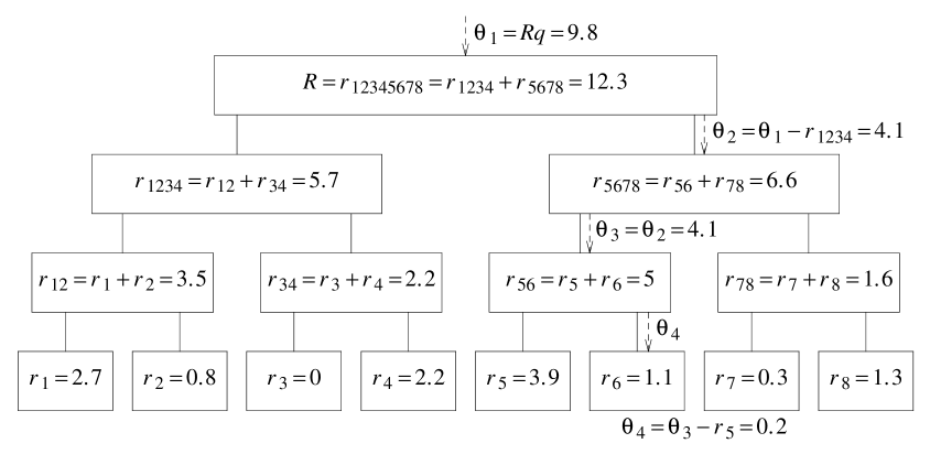
Figure 4: Tracing down a binary dispenser tree with $N=8$ terminal nodes. An arrival of the aggregate process is delegated to a component process in $\text{log}_{2}(N)=3$ steps.

Better methods exist. Figure 4 exemplifies the binary tree method in which the component $i$ is found in $\text{log}_{2}(N)$ steps (if $N$ is a whole degree of 2; otherwise $\lceil\text{log}_{2}(N)\rceil$ steps). This method also starts with an independent sample $q$ of a random value uniformly distributed in $0<q<1$. Then, instead of a linear scan, a binary tree is traced to fit this value.

The tracing is started from the root which is entered with $\theta_{1}=Rq$. We then steer our way down the tree in $\text{log}_{2}(N)$ steps. At step $m+1$, having value $\theta_{m}$, $0\leq\theta_{m}<r_{1,..j,j+1,..k}$, we enter node with inscription $r_{i,..j,j+1,..k}=r_{i..j}+r_{j+1,..k}$ on it. If $\theta_{m}$ happens to be smaller than $r_{1,..j}$, then we go to the left branch $r_{1,..j}$ producing $\theta_{m+1}=\theta_{m}$. If $r_{1,..j}\leq\theta_{m}<r_{i,..j,j+1,..k}$, then we go to the right branch $r_{j+1,..k}$ producing $\theta_{m+1}=\theta_{m}-r_{1,...j}$.

To maintain current the weights on the tree, each time a rate $r_{i}$ changes, the contents of $\text{log}_{2}(N)+1$ nodes is updated. The update begins with the bottom node $i$, continues up, and terminates at the root.

A useful simulation run is the switching history of several thousand customers during a few simulated years. A time-driven version takes several computing hours to complete the run. The corresponding event-driven version with a Poisson dispenser implemented using the binary tree, takes several seconds. The latter version allows one to easily simulate markets of a much larger size while keeping the running time bearable. For example the behavior of a 100,000-customer market during several simulated years can be simulated in less than 2 minutes.

4.3 Ising spin simulations

Another application for the dispenser technique, is an Ising spin model [6] [2] in computational physics. As a computational mechanism, the Ising spin simulation is very similar to the econometric model of competition between the telephone providers which has been just discussed. $N$ ferromagnetic particles are in place of $N$ telephone customers. An external magnetic field pulling the particles so that they would align in the field’s direction plays the role of the economic incentive for customers to “align” their allegiance to the provider which gives best saving. And the additional local magnetic field around a particle when its neighbors have already aligned is analogous to the additional incentive for a customer to switch the provider when the customer’s calling parties have done so.

Specifically, the magnetic state called spin of each particle $i$, takes on two values, $s_{i}(t)=1$ or $s_{i}(t)=-1$. Depending on the current spins $s_{j}(t)$ of the near-neighbors $j$ of particle $i$, pulls to flip $s_{i}(t)=1$ to $-1$ and to flip $s_{i}(t)=-1$ to 1 are defined. The dependence involves external field direction and intensity. (The form of this dependence is not essential for the present discussion.) Similarly to the model discussed before, the flip mechanism is probabilistic. Simulation of the dynamics of Ising spins can thus be arranged using the efficient binary tree Poisson dispenser mechanism discussed above. In this method flipping one spin takes $\text{log}_{2}(N)$ computations.

One feature in the Ising model is different from the telephone competition model though. The Ising particles are arranged in a regular fashion. For example, they are placed in vertices of a two-dimensional square lattice where each particle has four near-neighbors: at the North, East, South, and West. By contrast, the calling volume matrix $v_{ij}$ which defines calling parties of a customer is not assumed to be regular. Because of the regularity in the Ising model, for any particle, there is only a small number of possible combinations of neighboring particle states. Let us count these combinations, say, for a planar square grid arrangement of the particles. Each of the North, East, South, and West spin can take on 2 values, which yields 16 combinations. The particle itself can be in the two spin states. Hence there are at most 32 different combinations each of which may define a different pull-to-flip rate. Therefore there are at most 32 different rates and this finite set is the same for all $N$ particles. (Examining the form in which the rate depends on the combination, this set further reduces to only 10 different rates [2].) Thus, each of the $N$ leaves in the dispenser tree contains one of a small number of possible values. The finiteness allows one [2] to improve the Poisson dispenser algorithm so that delegating one arrival of the aggregate process to a component process takes a constant amount of computations, instead of $\text{log}_{2}(N)$ computations.

5 Simulating sequential random update in parallel

Sequential random update is a general mechanism for modeling evolution of a multicomponent dynamic system. In this model, we consider a system with $N$ components, the state of the system is composed of states $s_{i}$ of its components, The system state changes at discrete instances $m=1,2,....$ according to the following cyclic procedure.

DO 1. Select a component $i$ randomly and uniformly in the range
$1\leq i\leq N$. 2. Change the state $s_{i}$ of the selected component. The new state $s_{i}^{m+1}$ is a function of the old state $s_{i}^{m}$ and perhaps the states of some other components $s_{j}^{m}$. 3. Increment $m$ by 1. UNTIL enough cycles are processed


Both the Ising spin model and the model of competition between telephone providers discussed in Section 4 fit the sequential random update scheme, if two transformations are made: 1) uniformizing the event arrival rates among the system components, 2) abandoning the continuous time and retaining only the update counter $m$.

The latter transformation is obvious. Let us explain the former one. We choose an upper bound $r_{*}$ on the event arrival rates $r_{i}(t)$ among the components. This can be easily done in the Ising model: $r_{*}$ is the largest among the finite number of possible rates $r_{i}$, see the discussion in Section 4.3. In the provider competition model, the most “unhappy” customer yields the upper bound on the switch rate.

We attribute the same rate $r_{*}$ to all components so that the components are selected with equal probability as required in Step 1 above. Suppose a component $i$ at Step 1 is selected. To compensate for the smaller rate with which the component $i$ is being updated, we make an additional coin toss and choose to update state $s_{i}$ in Step 2 with probability $r_{i}/r_{*}$. With the complimentary probability $1-r_{i}/r_{*}$ the state does not change. The no-change of state $s_{i}$ does not violate the format of the procedure; it is a special case of the update when $s_{i}^{m+1}=s_{i}^{m}$.

The model of circuit-switched wired network discussed in Section 3 almost fits this scheme, if we take $N(N-1)/2$ links between the switches as components and equate the number of occupied trunks on a link with the state of the component. If different node pairs $(n_{1},n_{2})$ have different call arrival rates, we uniformize the rates as in the previous two models. The feature that does not fit the scheme is that when a call request arrives between a node pair $(n_{1},n_{2})$ and is placed via node $\nu$ instead of the direct link, the state of components $(n_{1},\nu)$ and $(\nu,n_{2})$ is updated instead of the state of the original component $(n_{1},n_{2})$.

5.1 Ballistic particle deposition

Other instances of the sequential random update include cellular arrays and neural nets. We will now discuss an example [12] of a ballistic particle deposition. The deposition model is aimed at studying morphology of amorphous layers growing on planar substrates, the subject of interest to material scientists. In the model, spheres of equal diameters 1 are falling vertically down toward the flat horizontal surface, see an example in Figure 5.

Figure 5: First 100 particles deposited over a segment of length 10. Particle 1 was deposited first, then particle 2, and so on. The endpoints of the segment are “glued” together to form a circle. Because of this, the particles that fell close to a dashed boundary, like particle 1, are shown twice.

The deposition process is arranged as follows. Particles are deposited one at a time. To deposit a particle, first its center $x$ coordinate is sampled randomly and uniformly over the adsorbing range. The range is segment (0,10) in Figure 5. Different particles have their $x$ generated independently of each other. The initial height of the center, is chosen sufficiently high above the surface. Then the particle is falling vertically down until a contact occurs. For the particles that begin the process, the contact is likely to be with the adsorbing surface. Later in the process, a falling particle is more likely to contact a stationary one, deposited before. In either case, the first contact instantly stops the incoming particle thus defining its $z$ coordinate.

The ballistic deposition scheme is an instance of the random sequential update. We split the adsorbing range into sectors of equal measure (congruent segments in 2D or planar figures of equal area in 3D) and declare sectors to be the components of the system. The particle order index $m$ becomes the update order index. The state $s_{i}^{m}$ of component $i$ consists of the coordinates of those among the first $m$ particles, that have been deposited over sector $i$. That is, say in a two dimensional case, the $x$ of those particles centers must be in segment $i$.

A particle from sector $i$ but located close to the sector’s boundary may attach itself to a particle which was earlier deposited in sector $j$, $j\neq i$. That is how components/sectors $j$ may get involved in the state update of component $i$ in Step 2 of the sequential update scheme.

Whereas Figure 5 represents a small-scale “educational” example of deposition in two dimensions, interesting simulations are in three dimensions with two dimensional adsorbing range of a size larger than say 1000$\times$1000. Many millions if not billions of particles are supposed to be processed. Figure 6 presents particle density as a function of both time and height $z$ in a three dimensional deposition of 100 million particles. Running such an experiment on a workstation would take about a week of execution time. Can parallel processing be employed to speed up the deposition and other sequential update schemes?

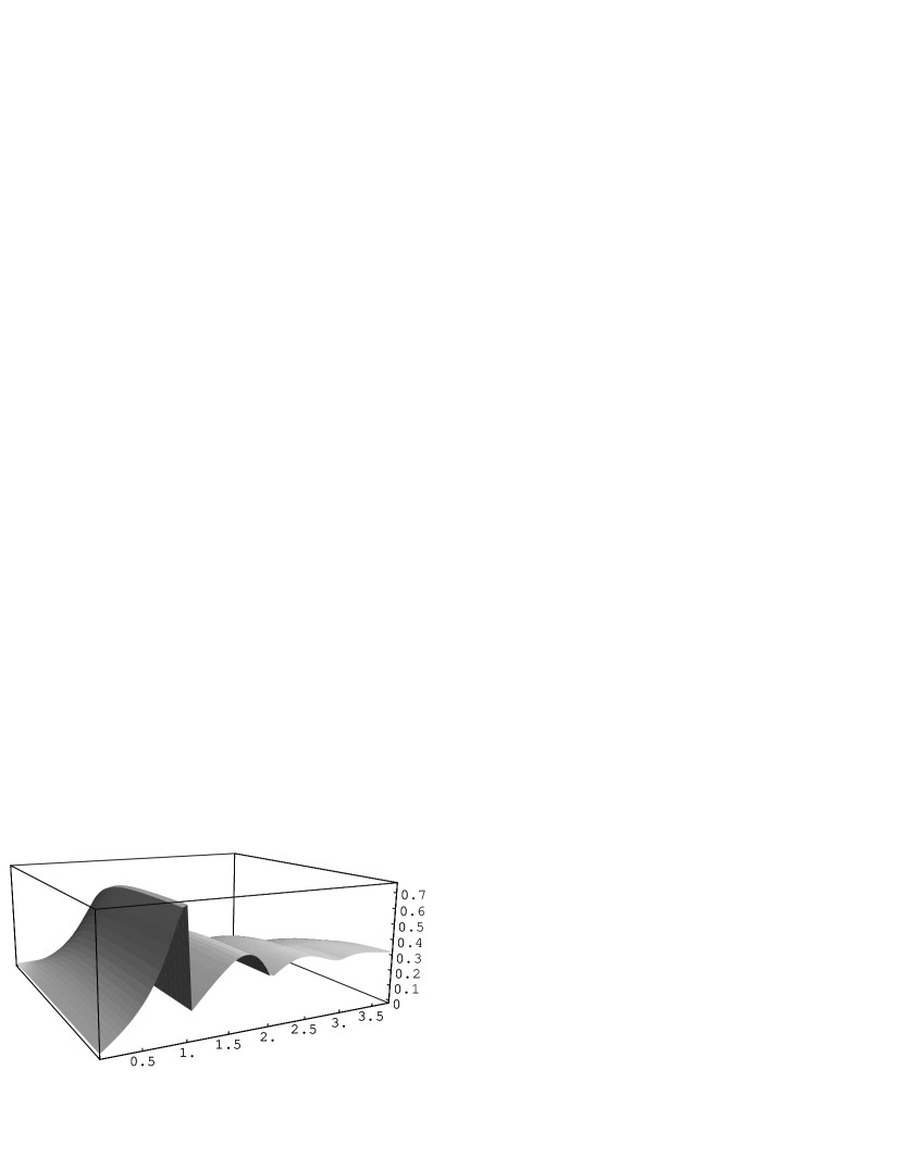
Figure 6: The density of deposited particles as a function of height and deposition time. The height, measured as $z-1/2$, is changing along the lower front horizontal edge of the box, the time is changing along the lower left horizontal edge. The rear facet of the box is the plane of zero time. The density is changing vertically.

5.2 Methods of parallelizing sequential random update

One idea of making the update scheme parallel may be to have a parallel computer dedicate $N$ processing elements (PEs) to the $N$ components of the system so that $\text{PE}_{i}$ would host component $i$, $i=1,2,...N$. The components would be updated concurrently without an organizing order. $\text{PE}_{i}$ would repeatedly update the state of component $i$, asynchronously obtaining from other PEs the current values of states of those components $j$ which are required for computing the new value of state of component $i$.

This proposal can be criticized from several viewpoints. The most basic objection is that it violates the standard model of reproducible computer execution. This entails various shortcomings. The generated trajectory of the system may be different from that generated sequentially. Say in the deposition example, the deposit structures generated in parallel may be statistically different from those generated sequentially. Moreover, the state change trajectories resulted in different runs of the same system with the same initial states, in general, will be different. This is very inconvenient as it makes both studying the obtained structures and debugging the simulation program very difficult.

Another proposal is to use $N+1$ PEs. A single “master” PE would be dedicated to dispensing the updates among the components. The $N$ “slave” PEs would host the $N$ components. A “slave” would be responsible for updating the state of the hosted component. Without further elaboration of the “master-slaves” scheme, we note that it can be organized so that the computations are reproducible and generate trajectories identical to those in the sequential procedure. Moreover, for a small number of PEs, the procedure may even be efficient. However, it does not scale for a large number of PEs. The sequential dispensing performed by the “master” becomes a bottleneck for a large $N$.

5.3 Cautious advancement method

In the example of ballistic deposition, we now describe another method of running the sequential random update scheme in parallel. Unlike the “chaotic” and the “master-slaves” methods, this method possesses both desirable properties: it generates a reproducible, correct simulated trajectory, and its good performance scales to a large size systems and large number $N$ of PEs.

The first step of the method is a reformulation of the sequential random update scheme in continuous time. In the old formulation the components are updated at discrete instances $m=1,2...$. In the new formulation the components are updated at instances $t_{1},t_{2},...t_{m},...$ of the continuous time, the instances constitute a Poisson process. An arbitrary positive $\lambda$ is chosen and fixed. The rate of the Poisson process is $N\lambda$. It follows, that each of the $N$ component processes also has arrivals that form a Poisson process. The component processes will be mutually independent. The rate of each component process will be $\lambda$.

Of course, in the Ising spins simulation model and in the provider competition model we have the Poisson processes to start with. We can reuse them with their original rates for the purpose of rendering the models in parallel. However, in the deposition model, the Poisson process is an additional structure, introduced only for the purpose of running the model in parallel.

In the Poisson dispenser method discussed in Section 4, we aggregated arrivals of individual components into a single stream which was to be sampled by the sequential computer. Here we do the opposite, namely, disaggregate the summary Poisson arrival stream into the independent streams of the components and let each component $i$ stream be sampled by a separate $\text{PE}_{i}$ which would be also responsible for maintaining state $s_{i}$ of component $i$.

Let $t^{i}$ denote the Poisson clock maintained by $\text{PE}_{i}$. That is, changes of state $s_{i}$ occur at time instances $t_{1}^{i},t_{2}^{i},....$. In the beginning of simulation each $\text{PE}_{i}$ sets its Poisson clock $t^{i}$ to 0 and has $s_{i}$ assume its initial value. Then each $\text{PE}_{i}$ asynchronously from other PEs executes the following procedure, which can be called “cautious advancements.”

DO 1. Sample next arrival $t_{i}$ of the Poisson process with rate $\lambda$. 2. If changing state $s_{i}$ at time $t_{i}$ requires the values $s_{j}$ of states of other components $j$, then wait until each such component $j$ reaches time $t_{j}$ so that it will become $t_{j}\geq t_{i}$. 3. Change the state $s_{i}$ of the hosted components as required, possibly using current values of states $s_{j}$ of other components $j$. UNTIL the simulation of component $i$ is completed


The PEs may execute this procedure with no other synchronization than that in the wait statement in Step 2, which is supposed to assure the “cautious advancement” of local times $t_{i}$. Because of the asynchrony, it might be not obvious that the procedure is correctly defined, let alone works correctly. For example, if concurrently with $\text{PE}_{i}$ updating $s_{i}$ and using state values $s_{j}$, $\text{PE}_{j}$ is changing $s_{j}$, is the state update in Step 3 well defined?

It was shown [11] that the cautious advancement scheme is correctly defined, works and is correct. Specifically, with probability 1, during an update of state $s_{i}$, other states $s_{j}$, the values of which are used in the $s_{i}$ update, are not themselves being changed. Cautious advancement is deadlock-free: no PE waits forever in Step 2. The sequence of updates obtained by merging the sequences of component updates generated by each PE is statistically identical to the sequence generated by the sequential procedure.

Reproducibility also takes place: if the cautious advancement procedure is executed twice with the same initial settings, including the same seeds of pseudorandom number generators, used for sampling Poisson arrivals, then the two resulting sequences of state updates will be identical with probability 1. This is despite that execution timings in different runs may be different.

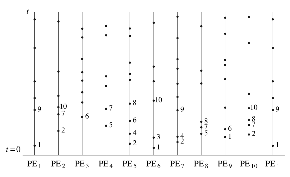
Figure 7: Local time lines of 10 processing elements that collectively perform a sequential random update, e.g., the particle deposition as in Figure 5. Dots mark the state update instants, e.g., instants when particles are deposited. The indices near the dots indicate the cycles when the updates occur

To get insight into the behavior of the cautious advancements, consider a simple example presented in Figure 7. Time lines of 10 components of a simulated model are depicted. For concreteness, we assume that the model represents the deposition of unit diameter circular particles over the segment of length 10 as in Figure 5. In the latter case, the substrate segment (0,10) is divided into 10 smaller segments: [0,1),[1,2),…[9,10). Segment [$i-1,i$) is component $i$ and it is hosted by $\text{PE}_{i}$.

Dots on the time lines mark the Poisson arrivals. At each arrival to segment [$i-1,i$), a particle with coordinate $x$, $i-1\leq x<i$, is deposited. Given that both the particle diameter and component segment length are unity, to know the landing height of the particle, there is no need to know positions of particles previously deposited over segments that are more than one component-segment away. However, a caution is exercised with respect to the immediate left and right neighbors of segment [$i-1,i$). $\text{PE}_{i}$ only deposits a particle at time $t_{i}$ if its two neighbors advanced their simulated times to reach or exceed $t_{i}$.

The immediate left neighbor is segment [$i-2,i-1$), unless $i=1$. The immediate right neighbor is segment [$i,i+1$), unless $i=N$. Points 0 and 10 representing the same point, the immediate left neighbor of component 1 is component $N$, whose immediate right neighbor is component 1. To be able to relate the arrival times for neighbors 1 and $N$, the time line of component 1 is drawn twice.

Although no additional synchronization is necessary for correctness and efficiency of the general cautious advancement procedure, it would help in understanding the procedure of deposition, if we assume that it is executed in lockstep. That is, no PE executes Step 2, before Step 1 is completed by all the PEs that are non-waiting at Step 2 of a preceding cycle. Then, in Step 2, all PEs check the simulated times achieved by their neighbors. As a result, the set of all PEs splits into those able to proceed further, and the rest which must wait. The non-waiting PEs begin Step 3 only after all PEs have finished the checking in Step 2. Finally, the new cycle by the non-waiting PEs begins not earlier, than all the non-waiting PEs have updated their state, i.e., deposited a particle.

The lockstep execution enables us to say at which cycle each state update occurs, that is, each particle gets deposited. In the situation of Figure 7, $\text{PE}_{1}$, $\text{PE}_{6}$, and $\text{PE}_{9}$ are lucky to process an event at cycle 1, while the rest of PEs are waiting. Values $t_{1},t_{6}$, and $t_{9}$ get advanced to the second arrival time and as a result $\text{PE}_{2}$, $\text{PE}_{5}$, $\text{PE}_{7}$, and $\text{PE}_{10}$ can process their events at cycle 2. Values $t_{2},t_{5},t_{7}$, and $t_{10}$ get advanced to the second arrival time and as a result $\text{PE}_{6}$ is lucky again and processes its second event.

In Figure 7, the cycle-per-event assignment is followed up to cycle 10. As an exercise, the reader may continue the task for the following cycles. The computational efficiency is determined by the fraction of non-waiting PEs at each cycle. This fraction is close to 25% on average in the example shown. Looking at the picture it seems likely that the fraction remains bounded from below and separated from zero when the size of the system gets larger and number of PEs increases proportionally. Mathematical studies [5] of this assertion confirm it in a general case. This means scalability of the parallel simulation performed by the cautious advancement mechanism. Using additional methods [12], in particular, allowing one PE to hold a larger sector or segment, the efficiency can be substantially increased, e.g., from 25% to 60% and higher. The mentioned above 100 million particle deposition experiment was run on a Maspar MP-1216 computer with 16,384 PEs. The run took 620 seconds (instead of a week on a workstation).

It becomes clear from the deposition example, that the efficiency of the cautious advancement parallel method for sequential random update depends on the topology of the connections among the components. The sparse fixed connections and a large diameter of the connection graph increase the efficiency. A small-diameter graph with all-to-all connections or close to such makes the PEs to be too cautious; too few of them would be non-waiting. In the worst case only one PE dares to advance the local time during a cycle while all the other PEs are cautiously waiting.

That is the case in the circuit-switched network simulation, where node pairs $(n_{1},n_{2})$ are close to each other in the sense of network connectivity. Even if we somehow resolved the difficulty that this model does not completely fit the random sequential update model as discussed in the beginning of the section, its parallel execution by the described method would not be efficient. However, the actual event dependency along the executional path is rather sparse which presents an opportunity for parallelism. Unfortunately, this parallelism is not extracted by the cautious advancement method, because the method requires a variable event dependency graph to be upper bounded by the fixed component connectivity graph.

Ising model and the phone provider competition model have a sparse component connectivity, but they still may fail to produce an efficient simulation using the described technique. This is because, for example in the Ising model, among the parameters the spin flip rate depends on is the temperature [6], and a low temperature causes the ratio between a particle update rate and its upper bound to be large. Even though a high enough fraction of PEs do not wait with processing their events, most of the processed events are trivial time advancements without a flip. This ruins the efficiency of the parallel execution in low temperature regimes.

A successful use of the cautious advancement technique and its further developments for an Ising model at a non-very-low temperature has been demonstrated [9] with the model running on 400 PEs of a parallel supercomputer T3E and yielding a speedup of 260. Another example is a wireless simulation [4] where the calls are dynamically arriving at random positions in the service area according to a fixed distribution and the users are not moving during the calls. With such assumptions it is possible to arrange a variant of efficient cautious advancement parallel processing.

Next section discusses an alternative method of parallel execution. It aims to extract parallelism as it emerges during the execution rather than relying on a worst case estimate given by the connectivity graph. Also it needs no uniformization of the event arrival rates.

6 Synchronous relaxation

As in Section 5, we consider a discrete event simulation of a dynamic system with $N$ components. The simulation is to be performed on a parallel computer with $N$ processing elements. As before, the procedure is to give each PE a component to host, and have the PE produce the state change history of that component. The method to do so will be different from the one discussed in Section 5. Unlike the previous method in which the event processing is final, the present method involves speculative computations wherein an event can be processed and then later rejected. The procedure was called synchronous relaxation[3].

In this procedure, each PE keeps track of the simulated time before which no event is to be rejected in the course of further processing; this quantity is called committed time. The PEs increase the committed time in lockstep, its value is common to all PEs. Each step consists of several iterations. At each iteration, while the committed time value does not change, each PE produces a speculative state change trajectory of the component it hosts beyond the committed time. The PE extends the trajectory until its local time reaches the committed time plus $\Delta t$, where $\Delta t$ is the step size of committed time increases. Unlike the $\Delta t$ of a time-driven simulation discussed in Section 2, here $\Delta t$ does not define the accuracy of simulation and may be not small.

Since components are, in general, connected, to produce a correct trajectory of its component, a PE needs to know the correct histories of other components. But they are not known, because other PEs are in the same quandary. The mechanism of generating the correct trajectories is by iterations. During the first iteration, each PE makes the simplest assumption about the trajectories of the other components, for example, that the other trajectories are empty of events, i.e., states do not change. This will enable the PE to produce the hosted component trajectory.

After every PE generates the speculative trajectory for additional $\Delta t$ units, they compare the trajectories. This comparison phase is started only after all PEs have generated the trajectories. As a rule, a PE will detect inconsistencies between the assumed and actually generated trajectories of other components. If so, PEs perform more iterations.

During subsequent iterations, if a PE needs to know the trajectory of a component hosted by another PE, it uses the trajectory generated in the last iteration. The goal of producing correct trajectories at a step is achieved if no PE detects any inconsistencies between the assumed and actually generated trajectories of other PEs. Once this happens, all PEs increase committed time by $\Delta t$ and continue.

The synchronous relaxation parallel algorithm [3], used on a Maspar computer with 16,384 PEs, cuts the running time of simulating a circuit-switched wired network to a few minutes (from several hours in the best sequential implementation on a fast workstation).

Naturally, the efficiency of the synchronous relaxation method relies on the convergence to be achieved at each step in a small number of iterations. To assess the number of iterations we examine the event dependency graph. For the event chains like the one in Figure 8 there will be many iterations. Figure 8 depicts an artificially difficult, worst case example. Such event dependency graph may correspond to a single indivisible object which moves in space visiting the areas hosted by different PEs. It is not feasible to make an efficient parallel simulation in such a special example.

Figure 8: An event dependency graph which makes inefficient a parallel execution

Figure 9: Event dependency levels. The number of levels bounds from above the number of iterations of the synchronous relaxation

In Figure 9, on the other hand, an “average” example is presented. It is obtained by randomly “sprinkling” the events-circles and possible event dependency links on the time-space diagram, without a particular application in mind. A good upper bound on the number of iterations can be supplied by counting levels. The levels can be identified without knowing the system partitioning into components hence no such partitioning is shown in Figure 9. Level 0 consists of already processed events that are positioned below the $\Delta t$ strip. Level 1 consists of those events at or above the lower boundary of the strip, which are immediate effects of only level 0 events. By induction, level $k$ consists of the events at or above the lower boundary of the strip, whose immediate causes are events at levels $k-1,k-2,...1$. In addition, to qualify for being on level $k$, the event must have al least one event on level $k-1$ among its immediate causes.

Before the step begins, all level 0 events are correct. After all the PEs generate their trajectories at iteration 1, all level 1 events at least will be among the correctly settled events. It can be seen by induction that after iteration $k$, all events on level $k$ or lower are correct. Thus, the number of levels for those events of the event dependency graph that fit within the considered $\Delta t$-strip is an upper bound on the number of iterations needed for correctly determining all events for this strip.

The actual number of iterations can be smaller than this upper bound for two reasons: 1) initial guesses of events are correct, 2) the event dependency subgraph hosted by a PE contains a complete set of cause-effects for several levels without need to know events in the neighboring PEs. Situation 1 is not always negligibly rare: in the applications in which there are only two choices for an event, reasonable initial guessing might save iterations. An extreme case of situation 2 is completely independent subsystems hosted by different PEs, or, for that matter, just a single PE which hosts the entire system. In these conditions, all events are determined correctly at the first iteration.

The question remains: How many event levels fits in the $\Delta t$-strip on an “average”? A conjecture can be proposed which says, that, in a “generic” example, if $N$ tends to infinity, the “average” number of levels increases not faster than $\text{log}N$. This has been established in several applications, for example, in the simulation of circuit-switched networks [3].

One may notice a similarity of the synchronous relaxation algorithm and the Time Warp algorithm [7]. Indeed, both algorithms use speculative event processing. The Time Warp procedure can be qualified as an asynchronous relaxation. Instead of frequent synchronization, the original TW procedure allows each PE to proceed at its own pace, without explicitly synchronizing with other PEs. As a result of tighter synchronization, the synchronous relaxation performs better than the TW in a worst case. The TW is known to sometimes enter undesirable modes like rollback avalanche or cascading, which might slow down unduly even well parallelizable simulations. Unlike the synchronous relaxation, no mathematical guarantee of scalability of the TW algorithm to a large $N$ has been offered.

Whenever there is a choice between a method with speculative computations and a method without, if both methods should deliver a scalable parallel simulation, the non-speculative method should be taken because speculative computations always involve a heavy computing overhead. Sometimes for the same simulation model in some regimes one can do well without speculative computations, while in the other regimes one can not. Such is the Ising model example. The uniformization entails a heavy overhead only for a low temperature and then synchronous relaxation is warranted. For higher temperatures, the method discussed in Section 5 provides a reasonable alternative.

7 Conclusion

There are many aspects in computer simulations, such as visualization, user interface, convenience and efficiency of programming etc. The aspect which comes first in simulating large dynamic systems is that of computing efficiency. A lesson learned from experiences in such tasks is that computing efficiency is determined by the properties of the underlying computational technique whereas the choice of the best technique is not defined by the modeling area. The same algorithmic idea may work well across diverse applications and modeling areas. Another lesson is that no single “silver bullet” technique for efficient simulation has been offered thus far and that a concrete simulation model may need a combination of available techniques to work fast. Sometimes one has to modify the model to fit a good technique. Yet in other cases very substantial improvements in computing speed are achieved if a basic technique is modified or augmented to fit the application, rather than being used in a fixed “prepackaged” form.

References

- [1] S. Borst, S. Grandhi, C. Kahn, K. Kumaran, B. Lubachevsky, D. Sand, “Wireless Simulation and Self-Organizing Spectrum Management,” BLTJ, 2, No. 3, pp. 81–98, Summer 1997.
- [2] A.B. Bortz, M.H. Kalos, J.L. Lebowitz, “A New Algorithm for Monte Carlo Simulation of Ising Spin Systems,” J. Comput. Phys. 17, No. 1, pp. 10–18, 1975.
- [3] S. Eick, A.G. Greenberg, B.D. Lubachevsky, and A. Weiss, “Synchronous Relaxation for Parallel Simulation with Applications to Circuit Switched Networks,” ACM Trans. On Modeling And Computer Simulation 3, No. 4, pp. 287–314, 1993.
- [4] A.G. Greenberg, B.D. Lubachevsky, D.M. Nicol, and P.E. Wright, “Efficient Massively Parallel Simulation of Dynamic Channel Assignment Schemes for Wireless Cellular Communications,” Proc. 8th Workshop on Parallel and Distributed Simulation, PADS’94, Edinburgh, Scotland, UK, pp.187-194.
- [5] A.G. Greenberg, S. Shenker, and A.L. Stolyar, “Asynchronous Updates in Large Parallel Systems,” Proc. ACM SIGMETRICS, pp. 91–103, 1996.
- [6] F. Ising, “Beitag zur theorie des ferromagnetismus,” Z. Physik, 31, pp. 253-258, 1925.
- [7] D.R. Jefferson, “Virtual Time,” ACM Trans. Prog. Lang. Sys. 7, No. 3, pp.404-425, 1985.
- [8] D.E. Knuth, Fundamental Algorithms, The Art of Computer Programming” 1, Addison-Wesley, Reading, Mass. 1968.
- [9] G. Korniss, M. A. Novotny, and P. A. Rikvold, “Parallelization of a Dynamic Monte Carlo Algorithm: A Partially Rejection-Free Conservative Approach,” J. Comput. Phys. 153, pp.488-508, 1999.
- [10] P.B. Linhart, B.D. Lubachevsky, R. Radner, and M.J. Meurer, “‘Friends and Family’ and Related Pricing Strategies,” Proc. 2nd Russian-Swedish Control Conference, Aug. 1995, St.Petersburg State Technical University, Russia, pp. 192-196.
- [11] B.D. Lubachevsky, “Efficient Parallel Simulations of Asynchronous Cellular Arrays,” Complex Systems. 1, No.6, pp. 1099-1123, 1987.
- [12] B.D. Lubachevsky, V. Privman, and S. Roy, “Casting Pearls Ballistically: Efficient Massively Parallel Simulation of Particle Deposition,” J. Comput Phys. 126, pp. 152-164, 1996.
- [13] B.D. Lubachevsky, F.H. Stillinger, “Geometric Properties of Random Disk Packings,” J. Statis. Phys. 90, Nos 5/6, pp. 561-583, 1990.
- [14] D.C. Rapaport, “The Event Scheduling Problem in Molecular Dynamic Simulation,” J. Comput. Phys. 34, No. 2, pp. 184-201, 1980.
- [15] www.pack-any-shape.com