Mining Frequent Itemsets from Secondary Memory

Abstract

Mining frequent itemsets is at the core of mining association rules, and is by now quite well understood algorithmically. However, most algorithms for mining frequent itemsets assume that the main memory is large enough for the data structures used in the mining, and very few efficient algorithms deal with the case when the database is very large or the minimum support is very low. Mining frequent itemsets from a very large database poses new challenges, as astronomical amounts of raw data is ubiquitously being recorded in commerce, science and government.

In this paper, we discuss approaches to mining frequent itemsets when data structures are too large to fit in main memory. Several divide-and-conquer algorithms are given for mining from disks. Many novel techniques are introduced. Experimental results show that the techniques reduce the required disk accesses by orders of magnitude, and enable truly scalable data mining.

1 Introduction

Mining frequent itemsets is a fundamental problem for mining association rules [4, 5, 11, 13, 14, 17, 20, 18]. It also plays an important role in many other data mining tasks such as sequential patterns, episodes, multi-dimensional patterns and so on [6, 12, 10]. In addition, frequent itemsets are one of the key abstractions in data mining.

The description of the problem is as follows. Let $I=\{i_{1},i_{2},\ldots,i_{j},\ldots i_{n}\}$, be a set of items. Items will sometimes also be denoted $a,b,c,\ldots$. An $I$-transaction $\tau$ is a subset of $I$. An $I$-transactional database $\cal D$ is a finite bag of $I$-transactions. The support of an itemset $S\subseteq I$ is the proportion of transactions in $\cal D$  that contain $S$. The task of mining frequent itemsets is to find all $S$ such that the support of $S$ is greater than some given minimum support $\xi$, where $\xi$ either is a fraction in $[0,1]$, or an absolute count.

Most of the algorithms, such as Apriori [5], DepthProject [3], and dEclat [21] work well when the main memory is big enough to fit the whole database or/and the data structures (candidate sets, FP-trees, etc). When a database is very large or when the minimum support is very low, either the data structures used by the algorithms may not be accommodated in main memory, or the algorithms spend too much time on multiple passes over the database. In the First IEEE ICDM Workshop on Frequent Itemset Mining Implementations, FIMI ’03 [18], many well known algorithms were implemented and independently tested. The results show that “none of the algorithms is able to gracefully scale-up to very large datasets, with millions of transactions” [19].

At the same time very large databases do exist in real life. In a medium sized business or in a company big as Walmart, it’s very easy to collect a few gigabytes of data. Terabytes of raw data is ubiquitously being recorded in commerce, science and government. The question of how to handle these databases is still one of the most difficult problems in data mining.

A few researchers have tried to mine frequent itemsets from very large databases. One approach is by sampling. For instance, [16] picks a random sample of the database, finds all frequent itemsets from the sample, and then verifies the results with the rest of the database. This approach needs only one pass of the database. However, the results are probabilistic, meaning that some critical frequent itemsets could be missing.

Partitioning [15] is another approach for mining very large databases. This approach first partitions the database into many small databases, and mines candidate frequent itemsets from each small database. One more pass over the original database is then done to verify the candidate frequent itemsets. The approach thus needs only two database scans. However, when the data structures used for storing candidate frequent itemsets are too big to fit in main memory, a significant amount of disk I/O’s is needed for the disk resident data structures.

In [8, 9], Han et. al. introduce the FP-growth method, which uses two database scans for constructing an FP-tree from the database, and then mines all frequent itemsets from the FP-tree. Two approaches are suggested for the case that the FP-tree is too large to fit into main memory.

The first approach writes the FP-tree to disk, then mines all frequent sets by reading the frequency information from the FP-tree. However, the size of the FP-tree could be same as the size of the database, and for each item in the FP-tree, we need at least one FP-tree traversal. Thus the I/O’s for writing and reading the disk-resident FP-tree could be prohibitive.

The second approach projects the original database on each frequent item, then mines frequent itemsets from the small projected databases. One advantage of this approach is that any frequent itemset mined from a projected database is a frequent itemset in the original database. To get all frequent itemsets, we only need to take the union of the frequent itemsets from the small projected databases. This is in contrast to the partitioning approach, where all candidate frequent itemsets have to be stored and later verified by another pass of database. The biggest problem of the projection approach is that the total size of the projected databases could be too large, and there will be too many disk I/O’s for the projected databases.

Contributions

In this paper we consider the problem of mining frequent itemsets from very large databases. We adopt a divide-and-conquer approach. First we give three algorithms, the general divide-and-conquer algorithm, then an algorithm using naive projection, and an algorithm using aggressive projection. We also analyze the number of steps and disk I/O’s required by these algorithms.

In a detailed divide-and-conquer algorithm, called Diskmine, we use the highly efficient FP-growth* method [7] to mine frequent itemsets from an FP-tree in main memory. We describe several novel techniques useful in mining frequent itemsets from disks, such as the array technique, the item-grouping technique, and memory management techniques.

Finally, we present experimental results that demonstrate the fact that our Diskmine-algorithm outperforms previous algorithms by orders of magnitude, and scales up to terabytes of data.

Overview

The remainder of this paper is organized as follows. In Section 2 we introduce approaches for mining frequent itemsets from disks. Three algorithms are introduced and analyzed. Section 3 gives a detailed divide-and-conquer algorithm Diskmine, in which many novel optimization techniques are used. These techniques are also described in Section 3. Experimental results are given in Section 4. Section 5 concludes, and outlines directions for future research.

2 Mining from disk

How should one go about when mining frequent itemsets from very large databases residing in a secondary memory storage, such as disks? Here “very large” means that the data structures constructed from the database for mining frequent itemsets can not fit in the available main memory.

Basically, there are two strategies for mining frequent itemsets, the datastructures approach, and the divide-and-conquer approach.

The datastructures approach consists of reading the database buffer by buffer, and generate datastructures (i.e. candidate sets or FP-trees). Since the datastructure don’t fit into main memory, additional disk I/O’s are required. The number of passes and disk I/O’s required by the approach depends on the algorithm and its datastructures. For example, if the algorithm is Apriori [5] using a hash-tree for candidate itemsets [15], disk based hash-trees have to be used. Then the number of passes for the algorithm is same as the length of the longest frequent itemset, and the number of disk I/O’s for the hash-trees depend on the size of the hash-trees on disk.

The basic strategy for the divide-and-conquer approach is shown in Figure 1. In the approach, $|\mbox{$\cal D$}|$ denotes the size of the data structures used by the mining algorithm, and $M$ is the size of available main memory. Function mainmine is called if candidate frequent itemsets (not necessary all) can be mined without writing the data structures used by a mining algorithm to disks. In Figure 1, a very large database is decomposed into a number of smaller databases. If a “small” database is still too large, i.e, the data structures are still too big to fit in main memory, the decomposition is recursively continued until the data structures fit in main memory. After all small databases are processed, all candidate frequent itemsets are combined in some way (obviously depending on the way the decomposition was done) to get all frequent itemsets for the original database.

Procedure diskmine($\mbox{$\cal D$},M$)

if $|\mbox{$\cal D$}|\leq M$ then return mainmine( $\cal D$)

else decompose $\cal D$ into $\mbox{$\cal D$}_{1},\ldots\mbox{$\cal D$}_{k}$.

return combine diskmine($\,\mbox{$\cal D$}_{1},M$),

…. ,

diskmine($\,\mbox{$\cal D$}_{k},M$).

Figure 1: General divide-and-conquer algorithm for mining frequent itemsets from disk.

The efficiency of diskmine depends on the method used for mining frequent itemsets in main memory and on the number of disk I/O’s needed in the decomposition and combination phases. Sometimes the disk I/O is the main factor. Since the decomposition step involves I/O, ideally the number of recursive calls should be kept small. The faster we can obtain small decomposed databases, the fewer recursive call we will need. On the other hand, if a decomposition cuts down the size of the projected databases drastically, the trade-off might be that the combination step becomes more complicated and might involve heavy disk I/O.

In the following we discuss two decomposition strategies, namely decomposition by partition, and decomposition by projection.

Partitioning is an approach in which a large database is decomposed into cells of small non-overlapping databases. The cell-size is chosen so that all frequent itemsets in a cell can be mined without having to store any data structures in secondary memory. However, since a cell only contains partial frequency information of the original database, all frequent itemsets from the cell are local to that cell of the partition, and could only be candidate frequent itemsets for the whole database. Thus the candidate frequent itemsets mined from a cell have to be verified later to filter out false hits. Consequently, those candidate sets have to be written to disk in order to leave space for processing the next cell of the partition. After generating candidate frequent itemsets from all cells, another database scan is needed to filter out all infrequent itemsets. The partition approach therefore needs only two passes over the database, but writing and reading candidate frequent itemsets will involve a significant number of disk I/O’s, depending on the size of the set of candidate frequent itemsets.

We can conclude that the partition approach to decomposition keeps the recursive levels down to one, but the penalty is that the combination phase becomes expensive.

To get an easier combination phase, we adopt another decomposition strategy, which we call projection. Suppose for simplicity that there are four items, $a,b,c,$ and $d$, and let $\cal D$ be a database of transactions containing some or all of these items. We could then decompose $\cal D$ into for instance $\mbox{$\cal D$}_{ab}$ and $\mbox{$\cal D$}_{cd}$. Typically, we would do this when the descending order of frequency of the items is $a,b,c,d$. In $\mbox{$\cal D$}_{cd}$ we put all transactions containing at $c$ or $d$ (or both). In $\mbox{$\cal D$}_{ab}$ we put transactions containing $a$ or $b$ (or both), and for each transaction we store only the $a,b$-part. Thus we will have shorter transactions in $\mbox{$\cal D$}_{ab}$, and both $\mbox{$\cal D$}_{ab}$ and $\mbox{$\cal D$}_{cd}$ contain fewer transactions than $\cal D$. We can then recursively mine all frequent itemsets from $\mbox{$\cal D$}_{ab}$, and $\mbox{$\cal D$}_{cd}$. Since this decomposition is not a partition, the projected databases might not be that much smaller that the original database. The upside is though that the set of all frequent itemsets in $\cal D$ now simply is the union of the frequent itemsets in $\mbox{$\cal D$}_{ab}$ and $\mbox{$\cal D$}_{cd}$. This means that the combination phase in diskmining is a simple union.

To illustrate this decomposition, let $\cal D$ contain the transactions $\{a,b,d\},\{b,c,d\},\{a,c\}$ and $\{a,b\}$. Suppose the minimum support is 50%, then $\mbox{$\cal D$}_{cd}=\{\{a,b,d\},\{b,c,d\},\{a,c\}\}$, $\mbox{$\cal D$}_{ab}=\{\{a,b\},\{b\},\{a\},\{a,b\}\}$. From $\mbox{$\cal D$}_{cd}$, we get all frequent itemsets $\{d\},\{b,d\}$, and $\{c\}$. Note though $\{a\}$ and $\{b\}$ are also frequent in $\mbox{$\cal D$}_{cd}$, they’re not listed since they contain neither $c$ nor $d$. They will be listed in the frequent itemsets of $\mbox{$\cal D$}_{ab}$, which are $\{a\},\{b\}$, and $\{a,b\}$.

To analyze the recurrence and required disk I/O’s of the general divide-and-conquer algorithm when the decomposition strategy is projection, let us suppose that:

• The original database size is $D$ bytes.

• The data structure is an FP-tree.

• The FP-tree constructed from original database $\cal D$ is $T$, and its size is $|T|$ bytes.

• If a conditional FP-tree $T^{\prime}$ is constructed from an FP-tree $T$, then $|T^{\prime}|\leq c\cdot|T|$, for some constant $c<1$.

• The main memory mining method is the FP-growth method [8, 9]. Two database scans are needed for constructing an FP-tree from a database.

• The block size is $B$ bytes.

• The main memory available for the FP-tree is $M$ bytes

In the first line of the algorithm in Figure 1, if $T$ can not fit in memory, then projected databases will be generated. We assumed that the size of the FP-tree for a projected database is $c\cdot|T|$. If $c\cdot|T|\leq M$, function mainmine can be called for the projected database, otherwise, the decomposition goes on. At pass $m$, the size of the FP-tree constructed from a projected database is $c^{m}\cdot|T|$. Thus, the number of passes needed by the divide-and-conquer projection algorithm is $1+\lceil\log_{c}M/T\rceil$. Based on our experience and the analysis in [8, 9], we can say that for all practical purposes the number of passes will be at most two. For example, Let $D=100$ Giga and $T=10$ Giga, $M=1$ Giga, $c=10\%$. Then the number of passes is $1+\lceil\log_{0.1}2^{30}/(10\times 2^{30})\rceil$ = 2. In five passes we can handle databases up to 100 Terabytes. Namely, we get $1+\lceil\log_{0.1}2^{30}/(10\times 2^{40})\rceil$ = 5.

Assume that there are two passes, and that the sum of the sizes of all projected databases is $D^{\prime}$. There are two database scans for $\cal D$, one for finding all frequent single items, one for decomposition. Two scans need $2\times D/B$ disk I/O’s. The projected databases have to be written to the disks first, then later each scanned twice for building the FP-tree. This step needs $3\times D^{\prime}/B$ disk I/O’s. Thus, the total disk number of disk I/O’s for the general divide-and-conquer projection algorithm is at least

$$2\cdot D/B+3\cdot D^{\prime}/B.$$ (1)

Obviously, the smaller $D^{\prime}$, the better the performance.

One of the simplest projection strategies is to project the database on each frequent item, which we call naive projection. First we need some formal definitions.

Definition 1

Let $I$ be a set of items. By $I^{*}$ we will denote strings over $I$, such that each symbol occurs at most once in the string. If $\alpha$, $\beta$ are strings, and $i_{j}$ an item, then $\alpha.\beta$ denotes the concatenation of the string $\alpha$ with the string $\beta$.

For a string $\alpha$, we shall denote by $\{\alpha\}$, the set of items occurring in it.

Let $\cal D$ be an $I$-database. Then ${\mit freqstring}(\mbox{$\cal D$})$ is the string over $I$, such that each frequent item in $\cal D$ occurs in it exactly once, and the items are in decreasing order of frequency in $\cal D$.     

As an example, consider the $\{a,b,c,d\}$-database $\mbox{$\cal D$}=\{\{a,b,c\},\{a,b,c,d\},\{a,c\}\}$. If the minimum support is 60%, then ${\mit freqstring}(\mbox{$\cal D$})=acb$. Note that $\{acb\}=\{a,c,b\}$.

Definition 2

Let $\cal D$ be an $I$-database, and let ${\mit freqstring}(\mbox{$\cal D$})=i_{1}i_{2}\cdots i_{k}$. For $j\in\{1,\ldots,k\}$ we define $\mbox{$\cal D$}_{i_{j}}=\{\tau\cap\{i_{1},\ldots,i_{j}\}:i_{j}\in\tau,\tau\in\mbox{$\cal D$}\}.$

Let $\alpha\in I^{*}$. We define $\mbox{$\cal D$}_{\alpha}$ inductively: $\mbox{$\cal D$}_{\epsilon}=\mbox{$\cal D$}$, and let ${\mit freqstring}(\mbox{$\cal D$}_{\alpha})=i_{1}i_{2}\cdots i_{k}$. Then, for $j\in\{1,\ldots,k\}$, $\mbox{$\cal D$}_{\alpha.i_{j}}=\{\tau\cap\{i_{1},\ldots,i_{j}\}:i_{j}\in\tau,\tau\in\mbox{$\cal D$}_{\alpha}\}.$     

Obviously, $\mbox{$\cal D$}_{\alpha.i_{j}}$ is an $\{i_{1},\ldots,i_{j}\}$-database. The decomposition of $\mbox{$\cal D$}_{\alpha}$ into $\mbox{$\cal D$}_{\alpha.i_{1}}$, …, $\mbox{$\cal D$}_{\alpha.i_{k}}$ is called the naive projection.

Definition 3

Let $\alpha\in I^{*}$, $i_{j}\in I$, and let $\mbox{$\cal D$}_{\alpha.i_{j}}$ be an $I$-database. Then ${\mit freqsets}(\xi,\mbox{$\cal D$}_{\alpha.i_{j}})$ denotes the subsets of $I$ that contain $i_{j}$ and are frequent in $\mbox{$\cal D$}_{\alpha.i_{j}}$ when the minimum support is $\xi$. Usually, we shall abstract $\xi$ away, and write just ${\mit freqsets}(\mbox{$\cal D$}_{\alpha.i_{j}})$     

Lemma 1

Let $\mbox{$\cal D$}_{\alpha}$ be an $I$-database, and ${\mit freqstring}(\mbox{$\cal D$}_{\alpha})=i_{1}i_{2}\cdots i_{k}$. Then

$${\mit freqsets}(\mbox{$\cal D$}_{\alpha})=\bigcup_{j\in\{1,\ldots,k\}}{\mit freqsets}(\mbox{$\cal D$}_{\alpha.i_{j}})$$

Proof. ($\subseteq$-direction). Let $S\in{\mit freqsets}(\mbox{$\cal D$}_{\alpha})$, and suppose $i_{n}$ is the item in $S$ that is least frequent in $\mbox{$\cal D$}_{\alpha}$. Since $\mbox{$\cal D$}_{\alpha.i_{n}}$ is an $\{i_{1},\ldots,i_{n}\}$-database, and transactions in $\mbox{$\cal D$}_{\alpha}$ that contain item $i_{j}$ are all in $\mbox{$\cal D$}_{\alpha.i_{j}}$, if $S$ is frequent in $\mbox{$\cal D$}_{\alpha}$, then $S$ must be frequent in $\mbox{$\cal D$}_{\alpha.i_{j}}$.

($\supseteq$-direction). For any frequent itemset $S\in freqsets(\mbox{$\cal D$}_{\alpha.i_{j}})$, according to the definition, the support of any itemset in $\mbox{$\cal D$}_{\alpha.i_{j}}$ is not greater than the support of it in $\mbox{$\cal D$}_{\alpha}$. Therefore, $S$ must be frequent in $\mbox{$\cal D$}_{\alpha}$.     

Figure 2 gives a divide-and-conquer algorithm that uses naive projection. A transaction $\tau$ in $\mbox{$\cal D$}_{\alpha}$ will be partly inserted into $\mbox{$\cal D$}_{\alpha.i_{j}}$ if and only if $\tau$ contains $i_{j}$. The parallel projection algorithm introduced in [9] is an algorithm of this kind.

Procedure naivediskmine($\mbox{$\cal D$}_{\alpha},M$)

if $|\mbox{$\cal D$}_{\alpha}|\leq M$ then return mainmine($\;\mbox{$\cal D$}_{\alpha}$)

else let ${\mit freqstring}(\mbox{$\cal D$}_{\alpha})=i_{1}i_{2}\cdots i_{n}$

return naivediskmine$(\mbox{$\cal D$}_{\alpha.i_{1}},M)\;\cup$

$\ldots\;\cup$

naivediskmine$(\mbox{$\cal D$}_{\alpha.i_{n}},M)$.

Figure 2: A simple divide-and-conquer algorithm for mining frequent itemsets from disk

Let’s analyze the disk I/O’s of the algorithm in Figure 2. As before, we assume that there are two passes, that the data structure is an FP-tree, and that the main memory mining method is FP-growth. If in $\mbox{$\cal D$}_{\epsilon}$, each transaction contains on the average $n$ frequent items, each transaction will be written to $n$ projected databases. Thus the total length of the associated transactions in the projected databases is $n+(n-1)+\cdots+1=n(n+1)/2$, the total size of all projected databases is $(n+1)/2\cdot D\approx n/2\cdot D$.

There are two database scans for $\mbox{$\cal D$}_{\epsilon}$, one for finding all frequent single items, and one for decomposition. Two scans need $2\cdot D/B$ disk I/O’s. The projected databases have to be written to the disks first, then later scanned twice each for building an FP-tree. This step needs at least $3\cdot n/2\times D/B$. Thus, the total disk I/O’s for the divide-and-conquer algorithm with naive projection is

$$2\cdot D/B+n\cdot 3/2\cdot D/B$$ (2)

The recurrence structure of algorithm naivediskmine is shown in Figure 3. The reader should ignore nodes in the shaded area at this point, they represent processing in main memory.

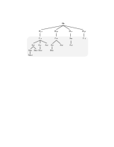
Figure 3: Recurrence structure of Naive Projection

In a typical application $n$, the average number of frequent items could be hundreds, or thousands. It therefore makes sense to devise a smarter projection strategy. Before we go further, we introduce some definitions and a lemma.

Definition 4

Let $\mbox{$\cal D$}_{\alpha}$ be an $I$-database, and let ${\mit freqstring}(\mbox{$\cal D$}_{\alpha})=\beta_{1}.\beta_{2}.\cdots.\beta_{k}$, where each $\beta_{j}$ is a string in $I^{*}$. We call $\beta_{1}.\beta_{2}.\cdots.\beta_{k}$ a grouping of ${\mit freqstring}(\mbox{$\cal D$}_{\alpha})$. For $j\in\{1,\ldots,n\}$, we now define $\mbox{$\cal D$}_{\alpha.\beta_{j}}=\{\tau\cap\{\beta_{1},\ldots,\beta_{j}\}:\tau\in\mbox{$\cal D$}_{\alpha},\tau\cap\beta_{j}\neq\emptyset\}.$

In $\mbox{$\cal D$}_{\alpha.\beta_{j}}$, items in $\{\beta_{j}\}$ are called master items, items in $\{\beta_{1},\ldots,\beta_{j-1}\}$ are called slave items.     

For example, if ${\mit freqstring}(\mbox{$\cal D$}_{\alpha})=abcde$, $\beta_{1}=abc$, $\beta_{2}=de$ gives the grouping $abc.de$ of $abcde$.

Definition 5

Let $\{\alpha,\beta\}\subset I^{*}$, and let $\mbox{$\cal D$}_{\alpha.\beta}$ be an $I$-database. Then $freqsets(\mbox{$\cal D$}_{\alpha.\beta})$ denotes the subsets of $I$ that contain at least one item in $\{\beta\}$ and are frequent in $\mbox{$\cal D$}_{\alpha.\beta}$.     

Lemma 2

Let $\alpha\in I^{*}$, $\mbox{$\cal D$}_{\alpha}$ be an $I$-database, and ${\mit freqstring}(\mbox{$\cal D$}_{\alpha})=\beta_{1}\beta_{2}\cdots\beta_{k}$. Then

$$freqsets(\mbox{$\cal D$}_{\alpha})=\bigcup_{j\in\{1,\ldots,k\}}freqsets(\mbox{$\cal D$}_{\alpha.\beta_{j}})$$

Proof. Straightforward from Lemma 1 and the definition of $\mbox{$\cal D$}_{\alpha.\beta}$.     

Based on Lemma 2, we can obtain a more aggressive divide-and-conquer algorithm for mining from disks. Figure 4 shows the algorithm aggressivediskmine. Here, ${\mit freqstring}(\mbox{$\cal D$}_{\alpha})$ is decomposed into several substrings $\beta_{j}$, each of which could have more than one item. Each substring corresponds to a projected database. A transaction $\tau$ in $\mbox{$\cal D$}_{\alpha}$ will be partly inserted into $\mbox{$\cal D$}_{\alpha.\beta_{j}}$ if and only if $\tau$ contains at least one item $a$ such that $a\in\{\beta_{j}\}$. Since there will be fewer projected databases, there will be less disk I/O’s. Compared with the algorithm in Figure 2, we can expect that a large amount of disk I/O will be saved by the algorithm in Figure 4.

Procedure aggressivediskmine($\mbox{$\cal D$}_{\alpha},M$)

if $|\mbox{$\cal D$}_{\alpha}|\leq M$ then return mainmine($\;\mbox{$\cal D$}_{\alpha}$)

else let ${\mit freqstring}(\mbox{$\cal D$}_{\alpha})=\beta_{1}\beta_{2}\cdots\beta_{k}$

return aggressivediskmine$(\mbox{$\cal D$}_{\alpha.\beta_{1}},M)\;\cup$

$\;\ldots\;\cup$

aggressivediskmine$(\mbox{$\cal D$}_{\alpha.\beta_{k}},M)$.

Figure 4: A more aggressive divide-and-conquer algorithm for mining frequent itemsets from disk

Let’s analyze the recurrence and disk I/O’s of the aggressive divide-and-conquer algorithm. The number of passes needed by the algorithm is still $1+\lceil\log_{c}M/T\rceil\approx 2$, since grouping items doesn’t change the size of an FP-tree for a projected database. However, for disk I/O, suppose in $\mbox{$\cal D$}_{\epsilon}$, each transaction contains on average $n$ frequent items, and that we can group them into $k$ groups of equal size. Then the $n$ items will be written to the projected databases with total length $n/k+2\cdot n/k+\ldots+k\cdot n/k=(k+1)/2\cdot n$. Total size of all projected databases is $(k+1)/2\cdot D\approx k/2\cdot D$. The total disk I/O’s for the aggressive divide-and-conquer algorithm is then

$$2\cdot D/B+k\cdot 3/2\cdot D/B$$ (3)

The recurrence structure of algorithm aggressivediskmine is shown in Figure 5. Compared to Figure 3, we can see that the part of the tree that corresponds to decomposition (the nonshaded part) is much smaller in Figure 5. Although the example is very small, it exhibits the general structure of the two trees.

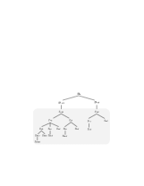
Figure 5: Recurrence structure of Aggressive Projection

If $k\ll n$, we can expect that the aggressive divide and conquer algorithm will significantly outperform the naive one.

3 Algorithm Diskmine

In this section we give the details of our divide-and-conquer algorithm for mining frequent itemsets from secondary memory. We call the algorithm Diskmine. In the algorithm, the FP-tree is used as data structure and the extension of FP-growth method, FP-growth* [7], as method for mining frequent itemsets from an FP-tree. Before introducing the algorithm, let’s first recall the FP-tree and the FP-growth* method.

3.1 The FP-tree and FP-growth* method

The FP-tree (Frequent Pattern tree) is a data structure used in the FP-growth method by Han et al.  [8]. It is a compact representation of all relevant frequency information in a database. The nodes of the FP-tree stores an item name, item count, and a link. Every branch of the FP-tree represents a frequent itemset, and the nodes along the branches are stored in decreasing order of the frequency of the corresponding items, with leaves representing the least frequent items. Compression is achieved by building the tree in such a way that overlapping itemsets share prefixes of the corresponding branches.

The FP-tree has a header table associated with it. Single items and their counts are stored in the header table in decreasing order of their frequency. The entry for an item also contains the head of a list that links all the nodes of the item in the FP-tree.

The FP-growth method needs two database scans when mining all frequent itemsets. The first scan counts the number of occurrences of each item. The second scan constructs the initial FP-tree, which contains all frequency information of the original dataset. Mining the database then becomes mining the FP-tree.

The FP-growth method relies on the following principle: if $X$ and $Y$ are two itemsets, the count of itemset $X\cup Y$ in the database is exactly that of $Y$ in the restriction of the database to those transactions containing $X$. This restriction of the database is called the conditional pattern base of $X$, and the FP-tree constructed from the conditional pattern base is called $X$’s conditional FP-tree, which we denote by $T_{X}$. We can view the FP-tree constructed from the initial database as $T_{\emptyset}$, the conditional FP-tree for $\emptyset$. Note that for any itemset $Y$ that is frequent in the conditional pattern base of $X$, the set $X\cup Y$ is a frequent itemset for the original database.

The recursive structure of FPgrowth can be seen from the shaded area in Figure 3. In the figure, we will enter the main memory phase for instance for the conditional database $\mbox{$\cal D$}_{a}$. Then FP-growth first constructs the FP-tree $T_{a}$ from $\mbox{$\cal D$}_{a}$. The tree rooted at $T_{a}$ shows the recursive structure of FP-growth, assuming for simplicity that the relative frequency remains the same in all conditional pattern bases.

In [7], we extend the FP-growth method into the FP-growth* method by using an array technique and other optimizations. The experimental results in the paper and those done by the FIMI-organizers show that the FP-growth* method outperforms the FP-growth method especially when the database is big or sparse [7, 18].

The array technique

In the original FP-growth method [8], to construct an FP-tree from a database $\cal D$, two database scan are required. The first scan gets all frequent items, the second constructs the FP-tree. And later, for each item $a$ in the header of a conditional FP-tree $T_{\alpha}$, two traversals of $T_{\alpha}$ are needed for constructing the new conditional FP-tree $T_{\alpha.i}$. The first traversal finds all frequent items in the conditional pattern base of $\alpha.i$, and initializes the FP-tree $T_{\alpha.i}$ by constructing its header table. The second traversal constructs the new tree $T_{\alpha.i}$.

In the boosted FP-growth* method [7], a simple data structure, an array, is introduced to omit the first scan of $T_{\alpha}$. This is achieved by constructing an array $A_{\alpha}$ while building $T_{\alpha}$. More precisely, in the second scan of the original database we construct $T_{\epsilon}$, and an array $A_{\epsilon}$. The array will store the counts of all 2-itemsets, each cell $[j,k]$ in the array is a counter of the 2-itemset $\{i_{j},i_{k}\}$. All cells in the array are initialized to 0. When an itemset is inserted into $T_{\epsilon}$, the associated cells in $A_{\epsilon}$ are updated. After the second scan, the array $A_{\epsilon}$ contains the counts of all pairs of items frequent in $\mbox{$\cal D$}_{\epsilon}$.

Next, the FP-growth* method is recursively called to mine frequent itemsets for each item in header table of $T_{\epsilon}$. However, now for each item $i$, instead of traversing $T_{\epsilon}$ along the linked list starting at $i$ to get all frequent items in $i$’s conditional pattern base, $A_{\epsilon}[i,*]$ gives all frequent items for $i$. Therefore, for each item $i$ in $T_{\epsilon}$ the array $A_{\epsilon}$ makes the first traversal of $T_{\epsilon}$ unnecessary, and $T_{\epsilon.i}$ can be initialized directly from $A_{\epsilon}$.

For the same reason, from a conditional FP-tree $T_{\alpha}$, when we construct a new conditional FP-tree for $\alpha.i$, for an item $i$, a new array $A_{\alpha.i}$ is calculated. During the construction of the new FP-tree $T_{\alpha.i}$, the array $A_{\alpha.i}$ is filled. The construction of arrays and FP-trees continues until the FP-growth method terminates.

Note that if for a database, if we have the array that stores the count of all pairs of frequent items, then only one database scan is needed to construct an FP-tree from the database.

3.2 Divide-and-conquer by aggressive projection

The algorithm Diskmine is shown in Figure 6. In the algorithm, $\mbox{$\cal D$}_{\alpha}$ is the original database or a projected database, and $M$ is the maximal size of main memory that can be used by Diskmine.

Procedure Diskmine$(\mbox{$\cal D$}_{\alpha},M)$

scan $\mbox{$\cal D$}_{\alpha}$ and compute freqstring$(\mbox{$\cal D$}_{\alpha})$

call ${\mit trialmainmine(\mbox{$\cal D$}_{\alpha},M)}$

if ${\mit trialmainmine(\mbox{$\cal D$}_{\alpha},M)}$ aborted then

compute a grouping $\beta_{1}\beta_{2}\cdots\beta_{k}$ of ${\mit freqstring}(\mbox{$\cal D$}_{\alpha})$.

Decompose $\mbox{$\cal D$}_{\alpha}$ into $\mbox{$\cal D$}_{\alpha.\beta_{1}},\ldots,\mbox{$\cal D$}_{\alpha.\beta_{k}}$

for j = 1 to k do begin

if $\{\beta_{j}\}$ is a singleton then

${\mit Diskmine}(\mbox{$\cal D$}_{\alpha.\beta_{j}},M)$

else

${\mit mainmine}(\mbox{$\cal D$}_{\alpha.\beta_{j}})$

end

else return freqsets$(\mbox{$\cal D$}_{\alpha})$

Figure 6: Algorithm Diskmine

Diskmine uses the FP-tree as data structure and FP-growth* [7] as main memory mining algorithm. Since the FP-tree encodes all frequency information of the database, we can shift into main memory mining as soon as the FP-tree fits into main memory.

Since an FP-tree usually is a significant compression of the database, our Diskmine algorithm begins optimistically, by calling trialmainmine, which starts scanning the database and constructing the FP-tree. If the tree can be successfully completed and stored in main memory, we have reached the bottom level of the recursion, and can obtain the frequent itemsets of the database by running FP-growth* on the FP-tree in main memory.

Procedure trialmainmine$(\mbox{$\cal D$}_{\alpha},M)$

start scanning $\mbox{$\cal D$}_{\alpha}$ and building the FP-tree

$T_{\alpha}$ in main memory.

if $|T_{\alpha}|$ exceeds $M$ then

return the incomplete $T_{\alpha}$

else

call FP-growth*$\,(T_{\alpha})$ and return freqsets$(\mbox{$\cal D$}_{\alpha})$.

Figure 7: Trial main memory mining algorithm

If, at any time during trialmainmine we run out of main memory, we abort and return the partially constructed FP-tree, and a pointer to where we stopped scanning the database. We then resume processing Diskmine$(\mbox{$\cal D$}_{\alpha},M)$ by computing a grouping $\beta_{1},\ldots,\beta_{k}$ of freqstring$(\mbox{$\cal D$}_{\alpha})$, and then decomposing $\mbox{$\cal D$}_{\alpha}$ into $\mbox{$\cal D$}_{\alpha.\beta_{1}},\ldots,\mbox{$\cal D$}_{\alpha.\beta_{k}}$. We recursively process each decomposed database $\mbox{$\cal D$}_{\alpha.\beta_{j}}$. During the first level of the recursion, some groups $\beta_{j}$ will consist of a single item only. If $\{\beta_{j}\}$ is a singleton, we call Diskmine, otherwise we call mainmine directly, since we put several items in a group only when we estimate that the corresponding FP-tree will fit into main memory.

In computing the grouping $\beta_{1},\ldots,\beta_{k}$ we assume that transactions in a very large database are evenly distributed, i.e., if an FP-tree is constructed from part of a database, then this FP-tree represents the whole FP-tree for the whole database. In other words, if the size of the FP-tree is $n$ for $p\%$ of the database, then the size of the FP-tree for whole database is $n/p\cdot 100$. Most of the time, this gives an overestimation, since an FP-tree increases fast only at the beginning stage, when items are encountered for the first time and inserted into the tree. In the later stages, the changes to the FP-tree will be mostly counter updates.

Procedure mainmine$(\mbox{$\cal D$}_{\alpha.\beta})$

build a modified FP-tree $T_{\alpha.\beta}$ for $\mbox{$\cal D$}_{\alpha.\beta}$

for each $i\in\{\beta\}$ do begin

construct the FP-tree $T_{\alpha.i}$ for $\mbox{$\cal D$}_{\alpha.i}$ from $T_{\alpha.\beta}$

call FP-growth*$\,(T_{\alpha.i})$ and return freqsets$(\mbox{$\cal D$}_{\alpha.i})$.

end

Figure 8: Main memory mining algorithm

Since we know that there is only one master item in the database (for $\mbox{$\cal D$}_{\epsilon}$, no master item at all), an FP-tree is constructed without the master item. In Figure 8, since $\mbox{$\cal D$}_{\alpha.\beta}$ is for multiple master items, the FP-tree constructed from $\mbox{$\cal D$}_{\alpha.\beta}$ has to contain those master items. However, the item order is a problem for the FP-tree, because we only want to mine all frequent itemsets that contain master items. To solve this problem, we simply use the item order in the partial FP-tree returned by the aborted trialmainmine$(\mbox{$\cal D$}_{\alpha})$. This is what we mean by a “modified FP-tree” on the first line in the algorithm in Figure 8.

The entire recurrence structure of Diskmine can be seen in Figure 5. Compared to the naive projection in Figure 3 we see that since the aggressive projection uses main memory more effective, the decomposition phase is shorter, resulting in less I/O.

Theorem 1

Diskmine$(\mbox{$\cal D$})$ returns freqsets$(\mbox{$\cal D$})$.

Proof. The correctness of Diskmine can be derived from the correctness of the FP-growth* method in [7] and Lemma 2 in Section 2. In Diskmine, each item acts as master item in exactly one projected database. If a projected database is only for one master item $i_{j}$, the result of FP-growth* method or a recursive call of Diskmine will be $freqsets(\mbox{$\cal D$}_{i_{j}})$. If a projected database is for a set $\{\beta\}$ of master items, it contains all frequency information associated with the master items. Since in the FP-growth* method, the order of the items in an FP-tree doesn’t influence the correctness of the FP-growth* method, mainmine indeed returns only frequent itemsets that contain master item(s), i.e. mainmine gives the exact value of $freqsets(\mbox{$\cal D$}_{\alpha.\beta})$. According to Lemma 2, algorithm Diskmine then correctly outputs all itemsets in frequent the original database.     

3.3 Memory Management

Given a database $\mbox{$\cal D$}_{\alpha}$, to successfully apply the FP-growth* method, the basic main memory requirement is that the size of the FP-tree $T_{\alpha}$ constructed from $\mbox{$\cal D$}_{\alpha}$, is less than the available amount $M$ of main memory. In addition, we need space for the descendant conditional FP-trees that will be constructed during the recursive calls of FP-growth*.

Suppose the main memory requirement for $T_{\alpha}$ plus its descendant FP-trees is $m$. If $M<m$, but the difference $m-M$ is not very big, the FP-growth* method could still be run because the operating system uses virtual memory. However, there could be too many page swappings which takes too much time and makes FP-growth* very slow. Therefore, given $M$, for a very large database $\mbox{$\cal D$}_{\alpha}$, we have to stop the construction of the FP-tree $T_{\alpha}$ and the execution of FP-growth* method before all physical main memory is used up.

Another problem is that we will construct a large number of FP-trees. Since there can be millions of nodes in those FP-trees, inserting and deleting nodes is time consuming.

In the implementation of the algorithm, we use our own main memory management for allocating and deallocating nodes, and calculating the main memory we have already used. We assume that the main memory needed by an FP-tree is proportional to the number of nodes in the FP-trees. We also assume that the workspace needed for calling FP-growth*(T) method on an FP-tree is roughly 10% of the size of the FP-tree $T$. Here, 10% is a liberal assumption according to the experimental result in [8]. Later in this section, a more accurate value will be given. If the size of FP-tree is more than $0.9\cdot M$, we conclude that $M$ is not big enough to store whole FP-tree $T_{\alpha}$.

Since all memory for nodes in an FP-tree is deallocated after a call of FP-growth* ends, a chunk of memory is allocated for each FP-tree when we create the tree, and the chunk size is changeable. After generating all frequent itemsets from the FP-tree, the chunk is discarded, and all nodes in the tree are deleted. Thus we successfully avoid freeing nodes in FP-trees one by one, which would take too much time.

3.4 Applying the Array Technique

In Diskmine, the array technique is also be applied to save FP-tree traversals. Furthermore, when projected databases are generated, the array technique can save a great number of disk I/O’s.

Recall that in trialmainmine, if an FP-tree can not be accommodated in main memory, the construction stops. Suppose now we decided to stop scanning the database. Then later, after generating all projected databases, for a projected database with only one master item, two database scans are required to construct an FP-tree for the master item. The first scan gets all frequent items for the master item, the second scan constructs the FP-tree. For a projected database with several master items, though the FP-tree constructed from the database uses the modified item order (the order from the header of the FP-tree in the previous level of the recursion), to construct new FP-trees for the master items, two FP-tree traversals are needed. To avoid the extra scan, in Diskmine we calculate an array for each FP-tree. When constructing the FP-tree from $\mbox{$\cal D$}_{\alpha}$, if it is found that the tree can not fit in main memory, the construction of the FP-tree $T_{\alpha}$ stops, but the scan of the database $\mbox{$\cal D$}_{\alpha}$ continues so that we finish filling the cells of the array $A_{\alpha}$. Here, some extra disk I/O’s are spent, but the payback will be that we save one database scan for each projected database. Furthermore, finishing the scanning of $\mbox{$\cal D$}_{\alpha}$ doesn’t require any more main memory, since the array $A_{\alpha}$ is already there.

From the array, for each projected database, the count of each pair of master items and the count of each pair of master item and slave item can be known. As an example, suppose a projected databases is only for one master item $i_{j}$ and slave items $i_{1},\ldots,i_{j-1}$. To mine all frequent itemsets, from the line for $i_{j}$ in the array, accurate counts for $[i_{j},i_{j-1}],[i_{j},i_{j-2}],\ldots,[i_{j},i_{1}]$ can be easily found. If there were no array we would need an extra database scan.

With the array, we can also make a projected database drastically smaller. In the definition of $\mbox{$\cal D$}_{\alpha.\beta_{j}}$, we see that $\mbox{$\cal D$}_{\alpha.\beta_{j}}$ is an $\{\beta_{1},\ldots,\beta_{j}\}$-database. Actually, by checking the array $A_{\alpha}$, if a slave item is found not frequently co-occurring with any master item in $\beta_{j}$, it’s useless to include the slave item in $\mbox{$\cal D$}_{\alpha.\beta_{j}}$, because no frequent itemsets mined from $\mbox{$\cal D$}_{\alpha.\beta_{j}}$ will contain that slave item. For same reason, if we also find that a master item $a$ is not frequent with any other master item or slave item, it will be not written to $\mbox{$\cal D$}_{\alpha.\beta_{j}}$, either. However, the frequent itemset $\alpha.a$ is outputted. Furthermore, if from the array, we see that a master item $a$ is only frequent with one item (master or slave) $b$, frequent itemsets $\alpha.a$ and $\alpha.a.b$ are outputted directly, and item $a$ will not appear in $\mbox{$\cal D$}_{\alpha.\beta_{j}}$. Therefore, by looking through the array, we find all slave items, such that they are not frequent with any master item in $\beta_{j}$, and all master items, such that their number of frequent items in $\{\beta_{1},\ldots,\beta_{j}\}$ is 0 or 1. When generating $\mbox{$\cal D$}_{\alpha.\beta_{j}}$, all those items are removed from the transactions we put in $\mbox{$\cal D$}_{\alpha.\beta_{j}}$.

3.5 Statistics

$t(\mbox{$\cal D$}_{\alpha})$	Number of transactions in $\mbox{$\cal D$}_{\alpha}$
$A_{\alpha}[j,k]$	Count of frequent item pair $\{i_{j},i_{k}\}$ in $\mbox{$\cal D$}_{\alpha}$
$t(T_{\alpha})$	Number of transactions used for constructing $T_{\alpha}$
$\nu(T_{\alpha})$	Number of nodes in $T_{\alpha}$
$\nu[j](T_{\alpha})$	Number of nodes in $T_{\alpha}$ if we retain only nodes for items $i_{1},\ldots,i_{j}$
$\mu[j](T_{\alpha})$	Number of nodes in $T$, where a node $P$ for item $i_{k}$ is counted if
	it satisfies the following conditions: 1) $P$ is in a branch that contains $i_{j}$
	2) $i_{k}\in\{i_{1},\ldots,i_{j}\}$ 3) $A_{\alpha}[j,k]>\xi$

Table 1: Statistics Information

Algorithm Diskmine collects some statistics on the partial FP-tree $T_{\alpha}$ and the rest of database $\mbox{$\cal D$}_{\alpha}$, for the purpose of grouping items together. Table 1 shows the statistics information. In the table, $\mbox{$\cal D$}_{\alpha}$ is the original database or the current projected database, and freqstring($\mbox{$\cal D$}_{\alpha}$)= $i_{1}\ldots i_{j}\ldots i_{k}\ldots i_{n}$. The partial FP-tree is $T_{\alpha}$ and $\xi$ is the absolute value of the minimum support.

In the table, the array discussed in Section 3.4 is also listed as statistics. Values for the cells of the array are accumulated during the construction of the partial $T_{\alpha}$. If trialmainmine is aborted, the rest of the statistics is collected by scanning the remaining part of $\mbox{$\cal D$}_{\alpha}$. Values in $\nu[j](T_{\alpha})$ can also be obtained during the construction of $T_{\alpha}$. Here $\nu[j](T_{\alpha})$ records the size of the FP-tree after $T_{\alpha}$ is trimmed and only contains items $i_{1},\ldots,i_{j}$. Notice that $\nu(T_{\alpha})$ is equal to $\nu[n](T_{\alpha})$. This is also the size of a tree that can fit in main memory. The value for $\mu[j](T_{\alpha})$ can be obtained by traversing $T_{\alpha}$ once, it gives the size of the FP-tree $T_{\alpha.i_{j}}$.

It might seem that collecting all this statistics is a large overhead, however, since all work is done in main memory, it doesn’t take much time. And the time saved for disk I/O’s is far more than the time spent on gathering statistics.

3.6 Grouping items

In Figure 6, the fourth line computes a grouping $\beta_{1}\beta_{2}\cdots\beta_{k}$ of ${\mit freqstring}(\mbox{$\cal D$}_{\alpha})$. Each string $\beta$ corresponds to a group and each $\beta$ consists of at least one item. For each $\beta$, a new projected database $\mbox{$\cal D$}_{\alpha.\beta}$ will be computed from $\mbox{$\cal D$}_{\alpha}$, then written to disk and read from disk later. Therefore, the more groups, the more disk I/O’s. In other words, there should be as many items in each $\beta$ as possible. To group items, two questions have to be answered.

1. If $\beta$ currently only has one item $i_{j}$, after projection, is the main memory big enough for accommodating $T_{\alpha.i_{j}}$ constructed from $\mbox{$\cal D$}_{\alpha.i_{j}}$ and running the FP-growth* method on $T_{\alpha.i_{j}}$?

2. If more items are put in $\beta$, after projection, is the main memory big enough for accommodating $T_{\alpha.\beta}$ constructed from $\mbox{$\cal D$}_{\alpha.\beta}$ and running FP-growth* on $T_{\alpha.\beta}$ only for items in $\beta$?

Answering the first question is pretty easy, since for each item $i_{j}$, the number $\mu[j](T_{\alpha})$ gives the size of an FP-tree if the tree is constructed from the partial FP-tree $T_{\alpha}$. Therefore $\mu[j](T_{\alpha})$ can be used to estimate the size of FP-tree $T_{\alpha.i_{j}}$. By the assumption that the transactions in $\mbox{$\cal D$}_{\alpha}$ are evenly distributed and that the partial $T_{\alpha}$ represents the whole FP-tree for $\mbox{$\cal D$}_{\alpha}$, the estimated size of FP-tree $T_{\alpha.i_{j}}$ is $\mbox{$\mu[j](T_{\alpha})$}\cdot\mbox{$t(\mbox{$\cal D$}_{\alpha})$}/\mbox{$t(T_{\alpha})$}$.

Before answering the second question, we introduce the cut point from which the first group can be easily found.

Finding the cut point. Recall the order that FP-growth* uses in mining frequent itemsets. Starting from the least frequent item $i_{n}$, all frequent itemsets that contains $i_{n}$ are mined first. Then the process is repeated for $i_{n-1}$, and so on. Notice that when mining frequent itemsets for $i_{k}$, all frequency information about $i_{k+1},\ldots,i_{n}$ is useless. Thus, though a complete FP-tree $T_{\alpha}$ constructed from $\mbox{$\cal D$}_{\alpha}$ could not fit in main memory, we can find many $k$’s such that the trimmed FP-tree containing only nodes for items $i_{k},\ldots,i_{1}$ will fit into main memory. All frequent itemsets for $i_{k},\ldots,i_{1}$ can be then mined from one trimmed tree. We call the biggest of such $k$’s the cut point. At this point, main memory is big enough for storing the FP-tree containing only $i_{k},\ldots,i_{1}$, and there is also enough main memory for running FP-growth* on the tree. Obviously, if the cut point $k$ can be found, items $i_{k},\ldots,i_{1}$ can be grouped together. Only one projected database is needed for $i_{k},\ldots,i_{1}$.

There are two ways to estimate the cut point. One way is to get cut point from the value of $t(\mbox{$\cal D$}_{\alpha})$ and $t(T_{\alpha})$ in Table 1. Figure 9 illustrates the intuition behind the cut point. In the figure, since the partial FP-tree for $t(T_{\alpha})$ of $t(\mbox{$\cal D$}_{\alpha})$ transactions can be accommodate in main memory, we can expect that the FP-tree containing $i_{k},\ldots,i_{1}$, where $k=\lfloor n\cdot\mbox{$t(T_{\alpha})$}/\mbox{$t(\mbox{$\cal D$}_{\alpha})$}\rfloor$, also will fit in main memory.

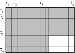
Figure 9: Cut Point. Here $l=\mbox{$t(T_{\alpha})$}$, and $m=\mbox{$t(\mbox{$\cal D$}_{\alpha})$}$

The above method works well for many databases, especially for those databases whose corresponding FP-trees have plenty of sharing of prefixes for items from $i_{1}$ to the cut point. However, if the FP-tree constructed from a database doesn’t share prefixes that much, the estimation could fail, since now the FP-tree for items from $i_{1}$ to the cut point could be too big. Thus, we have to consider another method. In Table 1, $\nu[j](T_{\alpha})$ records the size of the FP-tree after the partial FP-tree $T_{\alpha}$ is trimmed and only contains items $i_{1},\ldots,i_{j}$. Based on $\nu[j](T_{\alpha})$ the number of nodes in the complete FP-tree for item $i_{j}$ can be estimated as $\mbox{$\nu[j](T_{\alpha})$}\cdot\mbox{$t(\mbox{$\cal D$}_{\alpha})$}/\mbox{$t(T_{\alpha})$}$. Now, finding the cut point becomes finding the biggest $k$ such that $\nu[k](T_{\alpha})\cdot\mbox{$t(\mbox{$\cal D$}_{\alpha})$}/\mbox{$t(T_{\alpha})$}\leq\mbox{$\nu(T_{\alpha})$}$, and $\nu[k+1](T_{\alpha})\cdot\mbox{$t(\mbox{$\cal D$}_{\alpha})$}/\mbox{$t(T_{\alpha})$}>\mbox{$\nu(T_{\alpha})$}$.

Sometimes the above estimation only guarantees that the main memory is big enough for the FP-tree which contains all items between $i_{1}$ and the cut point, while it doesn’t guarantee that the descendant trees from that FP-tree can fit in main memory. This is because the estimation doesn’t consider the size of descendant trees correctly (in Section 3.3, we assumed that the size of a conditional tree is 10% of its nearest ancestor tree). Actually, from $\mu[j](T_{\alpha})$ we can get a more accurate estimation of the size of the biggest descendant tree. To find the cut point, we need to find the biggest $k$, such that $(\nu[k](T_{\alpha})+\mbox{$\mu[j](T_{\alpha})$})\cdot\mbox{$t(\mbox{$\cal D$}_{\alpha})$}/\mbox{$t(T_{\alpha})$}\leq\mbox{$\nu(T_{\alpha})$}$, and $(\nu[k+1](T_{\alpha})+\mu[m](T_{\alpha}))>\mbox{$\nu(T_{\alpha})$}$, where $j\leq k$, $\mbox{$\mu[j](T_{\alpha})$}={\mit max}_{j\in\{1,\ldots,k\}}\mbox{$\mu[j](T_{\alpha})$}$, and $m\leq k+1$, $\mu[m](T_{\alpha})={\mit max}_{m\in\{1,\ldots,k+1\}}\mu[m](T_{\alpha})$.

Grouping the rest of the items. Now we answer the second question, how to put more items into a group? Here we still need $\mu[j](T_{\alpha})$. Starting with $\mu[{\mit cutpoint}+1](T_{\alpha})$, we test if $\mu[{\mit cutpoint}+1](T_{\alpha})\cdot\mbox{$t(\mbox{$\cal D$}_{\alpha})$}/\mbox{$t(T_{\alpha})$}>\mbox{$\nu(T_{\alpha})$}$. If not, we put next item cutpoint+2 into the group, and test if $(\mu[{\mit cutpoint}+1](T_{\alpha})+\mu[{\mit cutpoint}+2](T_{\alpha}))$ $\cdot\mbox{$t(\mbox{$\cal D$}_{\alpha})$}/\mbox{$t(T_{\alpha})$}>\mbox{$\nu(T_{\alpha})$}$. We repeatedly put next item in ${\mit freqstring}(\mbox{$\cal D$})$ into the group until we reach an item $i_{j}$, such that

$$\sum_{m={\mit cutpoint}+1}^{j}\mu[m](T_{\alpha})\cdot\mbox{$t(\mbox{$\cal D$}_{\alpha})$}/\mbox{$t(T_{\alpha})$}>\mbox{$\nu(T_{\alpha})$}.$$

Then starting from $i_{j}$, we put items into next group, until all items find its group.

Why can we group items together? This is because even if we construct $T_{\alpha.i_{j}},\ldots,T_{\alpha.i_{k}}$ from the projected databases $\mbox{$\cal D$}_{\alpha.\beta_{i_{j}}},\ldots,\mbox{$\cal D$}_{\alpha.\beta_{i_{k}}}$ and put all of them into main memory, the main memory is big enough according to the grouping condition. At this stage, $T_{\alpha.i_{j}},\ldots,T_{\alpha.i_{k}}$ all can be constructed by scanning $\mbox{$\cal D$}_{\alpha}$ once. Then we mine frequent itemsets from the FP-trees. However, we can do better. Obviously $T_{\alpha.i_{j}},\ldots,T_{\alpha.i_{k}}$ overlap a lot, and the total size of the trees is definitely greater than the size of $T_{\alpha.\beta}$. It also means that we can put more items into each $\beta$, only if the size of $T_{\alpha.\beta}$ is estimated to fit in main memory. To estimate the size of $T_{\alpha.\beta}$, part of $T_{\alpha}$ has to be traversed by following the links for the master items in $T_{\alpha}$.

3.7 Database projection

After all items have found their groups, the original database will be projected to small databases according to Definition 4. To save disk I/O’s, three techniques can be used:

1. In a group $\beta$, if the number of master items is greater than half of the number of frequent items (this often happens in the group that contains cut point), then $\mbox{$\cal D$}_{\alpha.\beta}$ is not necessary computed. To mine all frequent itemsets, $T_{\alpha.\beta}$ can be directly constructed from $\mbox{$\cal D$}_{\alpha}$ by reading it once. This is because $\mbox{$\cal D$}_{\alpha.\beta}$ is not much smaller than $\mbox{$\cal D$}_{\alpha}$, while the disk I/O’s for reading from $\mbox{$\cal D$}_{\alpha}$ once is less than the disk I/O’s for writing and reading $\mbox{$\cal D$}_{\alpha.\beta}$ once.

2. Since the partial tree $T_{\alpha}$ now in main memory, records all frequency information of those transactions that have been read so far, when computing projected databases, the frequency information of those transactions can be gotten from $T_{\alpha}$. Thus disk I/O’s are only spent on reading from those transactions that did not contribute to $T_{\alpha}$.

3. As discussed in Section 3.4, by using the array technique, in group $\beta_{j}$, we find all slave items, such that they are not frequent with any master item in $\beta_{j}$, and all master items, such that their number of frequent items in $\{\beta_{1},\ldots,\beta_{j}\}$ is 0 or 1. When computing $\mbox{$\cal D$}_{\alpha.\beta_{j}}$, all those items are removed from new transactions in $\mbox{$\cal D$}_{\alpha.\beta_{j}}$.

3.8 The disk I/O’s

Let’s re-count the disk I/O’s used in Diskmine. From the first scan we get all frequent items in $\mbox{$\cal D$}_{\epsilon}$, which needs $D/B$ disk I/O’s. In the second scan we construct a partial FP-tree $T_{\epsilon}$, then continue scanning the rest database for statistics, which needs another $D/B$ disk I/O’s. Suppose then that $k$ projected databases have to be computed. According to Section 2, the total size of the projected databases is approximately $k/2\cdot D$. For computing the projected databases, the frequency information in $T_{\epsilon}$ is reused, so only part of $\mbox{$\cal D$}_{\epsilon}$ is read. We assume on average half of $\mbox{$\cal D$}_{\epsilon}$ is read at this stage, which means $1/2\cdot D/B$ disk I/O’s. Writing and later reading $k$ projected databases will take $2\cdot k/2\cdot D/B=k\cdot D/B$ disk I/O’s. Suppose all frequent itemsets can be mined from the projected databases without going to the third level. Then the total disk I/O’s is

$$3/2\cdot D/B+k\cdot D/B$$ (4)

Compared with formula 3, Diskmine saves at least $k/2\cdot D/B$ disk I/O’s, thanks to the various techniques used in the algorithm.

4 Experimental Evaluation and Performance Study

In this section, we present the results from a performance comparison of Diskmine with the Parallel Projection Algorithm in [9] and the Partitioning Algorithm introduced in [15]. The scalability of Diskmine is also analyzed, and the accurateness of our memory size estimations are validated.

As mentioned in Section 2, the Parallel Projection Algorithm is a naive divide-and-conquer algorithm, since for each item a projected database is created. For performance comparison, we implemented Parallel Projection Algorithm, by using FP-growth as main memory method, as introduced in [9]. The Partitioning Algorithm is also a divide-and-conquer algorithm. We implemented the partitioning algorithm by using the Apriori implementation [2]. We chose this implementation, since it was well written and easy to adapt for our purposes.

We ran the three algorithms on both synthetic datasets and real datasets. Some synthetic datasets have millions of transactions, and the size of the datasets ranges from several megabytes to several hundreds gigabytes. Without loss of generality, only the results for some synthetic datasets and a real dataset are shown here.

All experiments were performed on a 2.0Ghz Pentium 4 with 256 MB of memory under Windows XP. For Diskmine and the Parallel Projection Algorithm, the size of the main memory is given as an input. For the Partitioning Algorithm, since it only has two database scans and each main-memory-sized partition and all data structures for Apriori are stored into main memory, the size of main memory is not controlled, and only the running time is recorded.

We first compared the performance of three algorithms on synthetic dataset. Dataset T100I20D100K was generated from the application of [1]. The dataset has 100,000 transactions and 1000 items, and occupies about 40 megabytes of memory. The average transaction length is 100, and the average pattern length is 20. The dataset is very sparse and FP-tree constructed from the dataset is bushy. For Apriori, a large number of candidate frequent itemsets will be generated from the dataset. When running the algorithms, the main memory size was given as 128 megabytes. Figure 10(a) shows the experimental result. In the figure, “Naive Algorithm” represents the Parallel Projection Algorithm, and “Aggressive Algorithm” represents the Diskmine algorithm.

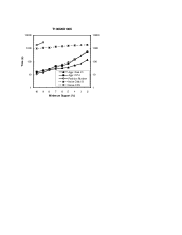
(a)

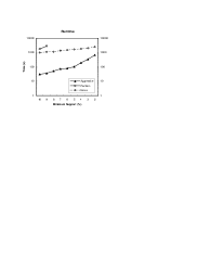
(b)

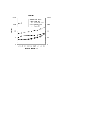
(c)

Figure 10: Experiments on Synthetic Data and Real Data

From Figure 10 (a), we can see that the Partitioning Algorithm is the slowest is the group. The Naive Algorithm, however, is not slower than the Aggressive Algorithm if we only compare their CPU time. In [7], where we concerned about main memory mining, we found that if a dataset is sparse the boosted FPgrowth* method has a much better performance than the original FProwth. The reason here the CPU time of the Aggressive Algorithm is not always less than that of Naive Algorithm is that the Aggressive Algorithm has to spend CPU time on calculating statistics. On the other hand, as expected, we can see in the figure that the disk I/O time of the Aggressive Algorithm is orders of magnitude smaller than that of the Naive Algorithm. In Figure 10 (b) we compare the total runnng times. We can see that the CPU overhead used by the Aggressive Algorithm now become insignificant compared to the savings in disk I/O.

We then ran the algorithms on a real dataset Kosarak, which is used as a test dataset in [18]. The dataset is about 40 megabytes. Since it is a dense dataset and its FP-tree is pretty small, we set the main memory size as 16 megabytes for the experiments. Results are shown in Figure 10 (c).

In Figure 10 (b), the Partitioning Algorithm is still the slowest. This is because it generates too many candidate frequent itemsets. Together with the data structures, these candidate sets use up main memory and virtual memory was used. We can also again notice that the CPU time of the Naive Algorithm is less than that of the Aggressive Algorithm. This is because Kosarak is a dense dataset so the array technique doesn’t help a lot. In addition, calculating the statistics takes much time. The disk I/O’s for the Aggressive Algorithm are still remarkably fewer than the disk I/O’s for the Naive Algorithm.

To test the effectiveness of the techniques for grouping items, we run Diskmine on T100I20D100K and see how close the estimation of the FP-tree size for each group is to its real size. We still set the main memory size as 128 megabytes, the minimum support is 2%. When generating the projected databases, items were grouped into 7 groups (the total number of frequent items is 826). As we can see from Figure 11 (a), in all groups, the estimated size is always slightly than the real size. Compared with the Naive Algorithm, which constructs an FP-tree for each item from its projected database, the Aggressive Algorithm almost fully uses the main memory for each group to construct an FP-tree.

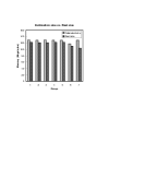
(a)

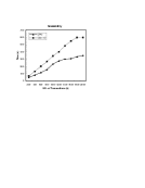
(b)

Figure 11: Estimation Effect and Scalability of Diskmine

As a divide-and-conquer algorithm, one of the most important properties of Diskmine is its good scalability. We ran Diskmine on a set of synthetic datasets. In all datasets, the item number was set as 10000 items, the average transaction length as 100, and the average pattern length as 20. The number of the transactions in the datasets varied from 200,000 to 2,000,000. Datasets size ranges from 100 megabytes to 1 gigabyte. Minimum support was set as 1.5%, and the available main memory was 128 megabytes. Figure 11 (b) shows the results. In the figure, the CPU and the disk I/O time is always kept in a small range of acceptable values. Even for the datasets with 2 million transactions, the total running time is less than 1000 seconds. Extrapolating from these figures using formula (4), we can conclude that a dataset the size of the Library of Congress collection (25 Terabytes) could be mined in around 18 hours with current technology.

5 Conclusions

We have introduced several divide-and-conquer algorithms for mining frequent itemset from secondary memory. We have analyzed the recurrences and disk I/O’s of all algorithms.

We then gave a detailed divide-and-conquer algorithm which almost fully uses the limited main memory and saves an numerous number of disk I/O’s. We introduced many novel techniques used in our algorithm.

Our experimental results show that our algorithm successfully reduces the number of disk access, sometimes by orders of magnitude, and that our algorithm scales up to terabytes of data. The experiments also validates that the estimation techniques used in our algorithm are accurate.

For future work, we notice that there are very few efficient algorithm for mining maximal frequent itemsets and closed frequent itemsets [13, 14, 17, 20] from very large databases. Unlike in Diskmine, where the frequent itemsets mined from all projected databases are globally frequent, a maximal frequent itemset or a closed frequent itemset mined from a projected database is only locally maximal or closed. As a challenge, a data structure, whose size may be also very big, must be set for recording all already discovered maximal or closed frequent itemsets. We also notice that our implementation of the partitioning algorithm is based on an existing Apriori implementation, which is not necessary highly optimized. As we know, there are situations when there are not too many candidate itemsets in a database, but the FP-tree constructed from the database is pretty big. In this situation the Partitioning Algorithm only needs two database scans and all frequent items can be nicely mined in main memory, or with very little I/O for keeping the candidate sets in virtual memory. In this situation Diskmine also needs two database scans, and it additionally needs to decompose the database. Therefore, exploring whether some clever disk-based datastructure would make the partition approach scale, is another interesting direction for further research.

References

- [1] www.almaden.ibm.com/software/quest
- [2] www.cs.helsinki.fi/u/goethals/software
- [3] R. C. Agarwal, C. C. Aggarwal and V. V. V. Prasad, Depth first generation of long patterns, In KDDM ’00, pp. 108-118
- [4] R. Agrawal, T. Imielinski, and A. Swami. Mining association rules between sets of items in large databases. In SIGMOD ’93, pp. 207–216, 1993.
- [5] R. Agrawal and R. Srikant. Fast algorithms for mining association rules. In VLDB ’94, pp. 487–499
- [6] R. Agrawal and R. Srikant. Mining sequential patterns. In ICDE ’95, pp. 3–14
- [7] G. Grahne, J. Zhu. Efficiently Using Prefix-trees in Mining Frequent Itemsets. In [19]
- [8] J. Han, J. Pei, and Y. Yin. Mining frequent patterns without candidate generation. In SIGMOD ’00, pp. 1–12
- [9] J. Han, J. Pei, Y. Yin and R. Mao. Mining frequent patterns without candidate generation: A Frequent-Pattern Tree Approach. In Data Mining and Knowledge Discovery, Vol. 8, pages 53-87, 2004.
- [10] M. Kamber, J. Han and J. Chiang. Metarule-Guided Mining of Multi-Dimensional Association Rules Using Data Cubes. In KDDM ’97, pp. 207–210
- [11] H. Mannila, H. Toivonen, and I. Verkamo. Efficient algorithms for discovering association rules. In KDDM ’94, pp. 181–192.
- [12] H. Mannila, H. Toivonen, and I. Verkamo. Discovery of Frequent Episodes in Event Sequences. In Data Mining and Knowledge Discovery. Volume 1, 3(1997), pages 259–289.
- [13] N. Pasquier, Y. Bastide, R. Taouil, and L. Lakhal. Discovering frequent closed itemsets for association rules. In ICDT’99, Jan. 1999.
- [14] J. Pei, J. Han and R. Mao, CLOSET: An Efficient Algorithm for Mining Frequent Closed Itemsets. In ACM SIGMOD Workshop on Research Issues in Data Mining and Knowledge Discovery, pages 21-30, 2000.
- [15] A. Savasere, E. Omiecinski, and S. Navathe. An efficient algorithm for mining association rules in large databases. In VLDB ’95, pp. 432–443
- [16] H. Toivonen. Sampling large databases for association rules. In VLDB ’96, pp. 134–145
- [17] J. Wang, J. Han, and J. Pei. CLOSET+: Searching for the Best Strategies for Mining Frequent Closed Itemsets. In Proc. 2003 ACM SIGKDD Int. Conf. on Knowledge Discovery and Data Mining (KDD’03), Washington, D.C., Aug. 2003.
-
[18]
B. Goethals and M. J. Zaki (Eds.)
Proceedings
of the First IEEE IDCM Workshop on Frequent Itemset Mining Implementations
(FIMI ’03).
CEUR Workshop Proceedings, Vol 80
http://CEUR-WS.org/Vol-90 - [19] Bart Goethals and Mohammed J. Zaki. Advances in Frequent Itemset Mining Implementations: Introduction to FIMI03. In 1st Workshop on Frequent Itemset Mining Implementations (FIMI’03) Melbourne, FL, Nov. 2003.
- [20] M. J. Zaki and C. Hsiao. CHARM: An Efficient Algorithm for Closed Itemset Mining. In Proceeding of The 2nd SIAM International Conference on Data Mining, Arlington, April 2002.
- [21] M. J. Zaki and Karam Gouda. Fast Vertical Mining Using Diffsets. In KDDM ’03, pp. 326–335