Neighborhood-Based Topology Recognition in Sensor Networks

Abstract

We consider a crucial aspect of self-organization of a sensor network consisting of a large set of simple sensor nodes with no location hardware and only very limited communication range. After having been distributed randomly in a given two-dimensional region, the nodes are required to develop a sense for the environment, based on a limited amount of local communication. We describe algorithmic approaches for determining the structure of boundary nodes of the region, and the topology of the region. We also develop methods for determining the outside boundary, the distance to the closest boundary for each point, the Voronoi diagram of the different boundaries, and the geometric thickness of the network. Our methods rely on a number of natural assumptions that are present in densely distributed sets of nodes, and make use of a combination of stochastics, topology, and geometry. Evaluation requires only a limited number of simple local computations.

ACM classification: C.2.1 Network architecture and design; F.2.2 Nonnumerical algorithms and problems; G.3 Probability and statistics

MSC classification: 68Q85, 68W15, 62E17

Keywords: Sensor networks, smart dust, location awareness, topology recognition, neighborhood-based computation, boundary recognition, Voronoi regions, geometric properties of sensor networks, random distribution.

1 Introduction

In recent time, the study of wireless sensor networks (WSN) has become a rapidly developing research area that offers fascinating perspectives for combining technical progress with new applications of distributed computing. Typical scenarios involve a large swarm of small and inexpensive processor nodes, each with limited computing and communication resources, that are distributed in some geometric region; communication is performed by wireless radio with limited range. As energy consumption is a limiting factor for the lifetime of a node, communication has to be minimized. Upon start-up, the swarm forms a decentralized and self-organizing network that surveys the region.

From an algorithmic point of view, the characteristics of a sensor network require working under a paradigm that is different from classical models of computation: Absence of a central control unit, limited capabilities of nodes, and limited communication between nodes require developing new algorithmic ideas that combine methods of distributed computing and network protocols with traditional centralized network algorithms. In other words: How can we use a limited amount of strictly local information in order to achieve distributed knowledge of global network properties?

This task is much simpler if the exact location of each node is known. Computing node coordinates has received a considerable amount of attention. Unfortunately, computing exact coordinates requires the use of special location hardware like GPS, or alternatively, scanning devices, imposing physical demands on size and structure of sensor nodes. A promising alternative may be continuous range modulation for measuring distances between nodes, but possible results have their limits: The accumulated inaccuracies from local measurements tend to produce significant errors when used on a global scale. This is well-known from the somewhat similar issue of odometry from the more progressed field of robot navigation, where much more powerful measurement and computing devices are used to maintaining a robot’s location, requiring additional navigation tools. See [SB03] for some examples and references. Finally, computation and use of exact coordinates of nodes tends to be cumbersome, if high accuracy is desired.

It is one of the main objectives of this paper to demonstrate that there may be a way to sidestep many of the above difficulties: Computing coordinates is not an end in itself. Instead, some structural location aspects do not depend on coordinates. An additional motivation for our work is the fact that location awareness for sensor networks in the presence of obstacles (i.e., in the presence of holes in the surveyed region) has received only little attention.

One key aspect of location awareness is boundary recognition, making sensors close to the boundary of the surveyed region aware of their position and letting them form connected boundary strips along each verge. This is of major importance for keeping track of events entering or leaving the region, as well as for communication purposes to the outside. Neglecting the existence of holes in the region may also cause problems in communication, as routing along shortest paths tends to put an increased load on nodes along boundaries, exhausting their energy supply prematurely; thus, a moderately-sized hole (caused by obstacles, by an event, or by a cluster of failed nodes) may tend to grow larger and larger.

Beyond discovering closeness to the boundary, it is desirable to determine the number and structure of boundaries, but also more advanced properties like membership to the outer boundary (which separates the region from the unbounded portion of the outside world) as opposed to the inner boundaries (which separate the swarm from mere holes in the region). Other important goals are the recognition of nodes that are well-protected by being far from the boundary, the recognition of nodes that are on the watershed between different boundaries (i.e., the Voronoi subdivision of the region), and the computation of the overall geometric thickness of the region, i.e., the size of the largest circle that can be fully inscribed into the region.

We show that based on a small number of natural assumptions, a considerable amount of location awareness can indeed be achieved in a large swarm of sensor nodes, in a relatively simple and self-organizing manner after deployment, without any use of location hardware. Our approach combines aspects of random distributions with natural geometric and topological properties.

Related Work. There are many papers dealing with node coordinates; for an overview, consider the cross-references for some of the following papers. A number of authors use anchors with known coordinates for computing node localization, in combination with hop count. See [DPG01, SRL02, SR02]. [ČHH01] uses only distances between nodes for building coordinates, based on triangulation. [PBDT03] presents a fully distributed algorithm that builds coordinate axes based on a by a near/far-metric and runs a spring embedder. Many related graph problems are NP-hard, as shown by [BK98] for unit disk graph recognition, and by [AGY04] for the case of known distances to the neighbors.

On the other hand, holes in the environment have rarely been considered. This is closely related to the $k$-coverage problem: Decide whether all points in the network area are monitored by at least $k$ nodes, where $k$ is given and fixed. In this context, a point is monitored by a node, if it is within the node’s sensing area, which in turn is usually assumed to be a disk of fixed size. By setting the sensing range to half the communication range, $1$-coverage becomes a decision problem for the existence of holes. In [HT03], an algorithm for $k$-coverage that can be distributed is proposed. Unfortunately, it requires precise coordinates for all nodes. In [FGG04], holes are addressed with greedy geographic routing in mind: Nodes where data packets can get stuck are identified using a fully local rule, allowing identification of the adjacent hole by using a distributed algorithm. Again, node coordinates must be known for both detection rule and bypassing algorithm to work. [Bea03] considers detection of holes resulting from failing nodes. It proposes a distributed algorithm that uses a hierarchical clustering to find a set of clusters that touch the failing region and circumscribe it.

Our Results. We show that distributed location awareness can be achieved without the help of location hardware. In particular:

• We describe how to recognize the nodes that are near the boundary of the region. The underlying geometric idea is quite simple, but it requires some effort on both stochastics and communication to make it work.

• We extend our ideas to distinguish the outside boundary from the interior boundaries.

• We describe how to compute both boundary distance for all nodes and overall region thickness.

• We sketch how to organize communication along the boundaries.

• We describe how to compute the Voronoi boundaries that are halfway between different parts of the boundary.

The rest of this paper is organized as follows. In Section 2 we give some basic notation and state our underlying model assumptions. In Section 3 we describe how to obtain an auxiliary tree structure that is used for computing and distributing global network parameters. Section 4 gives a brief overview of probabilistic aspects that are used in the rest of the paper to allow topology recognition. Section 5 describes how to perform boundary recognition, while Section 6 gives a sketch of how to compute more advanced properties. Section 7 describes implementation issues and shows some of our experiments. Finally, Section 8 discusses the possibilities for further progress based on our work.

2 Preliminaries

Swarm and geometry. In the following, we assume that the swarm consists of a set $V$ of nodes, and the cardinality of $V$ is some large number $n$. Each node $v\in V$ has a globally unique ID (for simplicity, denoted by $v$) of storage size $O(\log n)$, and coordinates $x_{v}$ that are unknown to any node. All node positions are contained in some connected region $A_{\mathrm{net}}\subset\mathbb{R}^{2}$, described by its boundary elements. In computational geometry, it is common to consider regions that are non-degenerate polygons, bounded by $k$ disjoint closed polygonal curves, consisting of a total of $s$ line segments, meeting pairwise in a total of $s$ corners. Each of the $k$ boundary curves separates the interior of $A_{\mathrm{net}}$ from a connected component of $\mathbb{R}^{2}\setminus A_{\mathrm{net}}$. The unique boundary curve separating $A_{\mathrm{net}}$ from the infinite component of $\mathbb{R}^{2}\setminus A_{\mathrm{net}}$ is called the outside boundary; all other boundaries are inside boundaries, separating $A_{\mathrm{net}}$ from holes. Thus, the genus of $A_{\mathrm{net}}$ is $k-1$. As we do not care about the exact shapes (and an explicit description of the boundary is neither required nor available to the nodes), we do not assume that $A_{\mathrm{net}}$ is polygonal, meaning that curved (e.g., circular) instead of linear boundary pieces are admissible; we still assume that it consists of $s$ elementary curves, joined at $s$ corners, with a total number of $k$ boundaries.

Figure 1: Geometric parameters.

As narrow bottlenecks in a region can lead to various computational problems, a standard assumption in computational geometry is to consider regions with a lower bound on the fatness of the region; for a polygonal region, this is defined as the ratio between $d_{\min}$, the smallest distance between a corner of the region and a nonadjacent boundary segment, and $d_{\max}$, the diameter of the region. When dealing with sensor networks, the only relevant parameter for measuring distances is the communication radius, $R$. Thus, we we use a similar parameter, called feature size, which is the ratio between $d_{\min}$ and $R$. For the rest of this paper, we assume that feature size has a lower bound of 2. (This technical assumption is not completely necessary, but it simplifies some matters, which is necessary because of limited space.) In addition, we assume that angles between adjacent boundary elements are bounded away from $0$ and from $2\pi$, implying that there are no sharp, pointy corners in the region.

Node distribution. A natural scenario for the deployment of a sensor network is to sprinkle a large number of small nodes evenly over a region. Thus, we assume that the positioning of nodes in the region is the result of a random process with a uniform distribution on $A_{\mathrm{net}}$. We also assume reasonable density; in a mathematical sense, this will be made clear further down. In a practical sense, we assume that each node can communicate with at least 100 other nodes, and the overall network is connected.

$\lambda(\cdot)$ denotes a volume function (i.e., the Lebesgue measure) on $\mathbb{R}^{2}$, therefore $0<\lambda(A_{\mathrm{net}})<\infty$. For simplicity, $\lambda_{\circ}:=\pi R^{2}$ denotes the area of the disk with radius $R$.

Using the notation $V(A):=\left\{v\in V:x_{v}\in A\right\}$, the expected number of nodes to fall into an area $A\subset A_{\mathrm{net}}$ is therefore

$$\mathrm{E}\!\left[\left|V(A)\right|\right]=n\frac{\lambda(A)}{\lambda(A_{\mathrm{net}})}\;.$$ (1)

Therefore, a node $v\in V$ that is not close to the network area’s boundary, i.e., $B_{R}(x_{v})\subset A_{\mathrm{net}}$ has an estimated neighborhood size of

$$\mu:=\mathrm{E}\!\left[\left|N(v)\right|\right]=(n-1)\frac{\lambda_{\circ}}{\lambda(A_{\mathrm{net}})}\;.$$ (2)

Here, $B_{r}(x)$ denotes the ball around $x$ with radius $r$.

Node communication. Nodes can broadcast messages that are received by all nodes within communication range. The cost of broadcasting one message of size $m$ is assumed to be $O(m)$; e.g., any message containing a sender ID incurs a cost of $O(\log n)$.

We assume that two nodes $u\neq v\in V$ can communicate if, and only if, they are within distance $R$. This is modeled by a set of edges, i.e., $uv\in E:\iff\left\|x_{u}-x_{v}\right\|\leqslant R$, where $\left\|\cdot\right\|$ denotes the Euclidean norm. The set of adjacent nodes of $v\in V$ is denoted by $N(v)$, and does not include $v$ itself. Such a graph is known under many names, e.g., geometric, (unit) disk, or distance graph. The maximum degree is denoted by $\Delta:=\max_{v\in V}\left|N(v)\right|$.

3 Leader Election and Tree Construction

A first step for self-organizing the swarm of nodes is building an auxiliary structure that is used for gathering and distributing data. The algorithms that are presented in Section 5 only work if certain global network parameters are known to all nodes. By using a directed spanning tree, nodes know when the data aggregation phase terminates and subsequent algorithmic steps may follow. This is in contrast to other methods like flooding, where termination time is unknown. The issue of leader election has been studied in various contexts; see [BKKM96] for a good description. In principle, protocols for leader election may be used for our purposes, as they implicitly construct the desired tree; however, using node IDs (or pre-assigning leadership) does offer some simplification.

An alternative to leader election is offered by the seminal paper [GHS83] dealing with distributed and emergent search tree construction. It builds a minimum spanning tree in a graph with $n$ nodes in a distributed fashion, using only local communication. Complexities are $O(n\log^{2}n)$ time from the first message by a node to completed information at the constructed root, and $O(\log^{2}n)$ transmissions per node, consisting of $O(\log n)$ messages, each sized $O(\log n)$.

In the following, we will use this auxiliary tree; in particular, we may assume that each node knows $N(v)$ and $n$, and it is able to use the tree for requesting and obtaining global data. Note that the tree is only used for bootstrapping the network; it may be replaced by a more robust structure at a later time.

4 Probabilistic Aspects

The idea for recognizing boundary nodes is relatively simple: Their communication range intersects a smaller than average portion of the region, and thus $N(v)$ is smaller than in other parts. However, a random distribution of nodes does not imply that the size of $N(v)$ is an immediate measure for the intersected area, as there may be natural fluctuations in density that could be misinterpreted as boundary nodes. In order to allow dealing with this difficulty, we introduce a number of probabilistic tools.

Recall that Chebychev’s inequality shows that for a binomial distribution for $n$ events with probability $p$, i.e., for a $\mathrm{bin}\left(n,p\right)$-distributed random variable $X$, and $\alpha<1$

$$\Pr\!\left[X\leqslant\alpha np\right]\leqslant\frac{1}{n}\cdot\mathrm{const}\to 0(n\to\infty)$$ (3)

holds. We exploit this fact to provide a simple local rule to let nodes decide whether they are close to the boundary $\partial A_{\mathrm{net}}$. Let $\alpha<1$ be fixed, and let

$$D=D(\alpha):=\left\{v\in V:\left|N(v)\right|\leqslant\alpha\mu\right\}\;.$$ (4)

Theorem 4.1

Let $v$ be a node whose communication range lies entirely in $A_{\mathrm{net}}$. Then $v\notin D$ with high probability.

Proof

This follows directly from (3), as

$$\Pr\!\left[\left|N(v)\right|\leqslant\alpha\mu\right]=\Pr\!\left[\left|V(B_{R}(x_{v}))\setminus\left\{v\right\}\right|\leqslant\alpha\mu\right]\to 0\quad(n\to\infty)\;.$$ (5)

∎

Theorem 4.2

Let $x\in\partial A_{\mathrm{net}}$ be on the network area’s boundary. Let $\varepsilon>0$. Assume $\alpha>\tfrac{1}{\lambda_{\circ}}{\lambda(B_{R+\varepsilon}(x)\cap A_{\mathrm{net}})}$. Then, with high probability, there is a node $v\in D$ with $\left\|x-x_{v}\right\|\leqslant\varepsilon$.

Proof

Let $A_{\varepsilon}\!\left(x\right):=B_{\varepsilon}(x)\cap A_{\mathrm{net}}$ be the area where $v$ is supposed to be. Then $\lambda(A_{\varepsilon}\!\left(x\right))>0$ by our assumption on feature size. The probability that there is no node in $A_{\varepsilon}\!\left(x\right)$ equals the probability for a $\mathrm{bin}\left(n,\tfrac{\lambda(A_{\varepsilon}\!\left(x\right))}{A_{\mathrm{net}}}\right)$-distributed variable to become zero, i.e.,

$$\Pr\!\left[\left|V(A_{\varepsilon}\!\left(x\right))\right|=0\right]=\left(1-\tfrac{\lambda(A_{\varepsilon}\!\left(x\right))}{A_{\mathrm{net}}}\right)^{n}\to 0\quad(n\to\infty)\;.$$ (6)

On the other hand, the probability that a node $u$ in $A_{\varepsilon}\!\left(x\right)$ has more than $\alpha\mu$ neighbors is

$$\Pr\!\left[\left|N(u)\right|>\alpha\mu\right] = \Pr\!\left[\left|V(A_{\varepsilon}\!\left(x\right))\right|>\alpha\mu+1\;\boldsymbol{|}\;u\mbox{ exists}\right]$$

$$\leqslant \Pr\!\left[\left|V(B_{R+\varepsilon}(x))\right|>\alpha\mu+1\right]$$

$$\to 0\quad(n\to\infty)\mbox{, because }\alpha\lambda_{\circ}>\lambda(A_{R+\varepsilon}\!\left(x\right))\;.$$

Together, we get

$$\Pr\!\left[\exists v\in V,x_{v}\in A_{\varepsilon}\!\left(x\right):\left|N(v)\right|\leqslant\alpha\mu\right]$$

$$= 1-\Pr\!\left[V(A_{\varepsilon}\!\left(x\right))=\varnothing\right]-\Pr\!\left[\forall v\in V(A_{\varepsilon}\!\left(x\right)):\left|N(v)\right|>\alpha\mu\;\boldsymbol{|}\;V(A_{\varepsilon}\!\left(x\right))\neq\varnothing\right]$$

$$\geqslant 1-\Pr\!\left[V(A_{\varepsilon}\!\left(x\right))=\varnothing\right]-\Pr\!\left[\left|N(v)\right|>\alpha\mu\;\boldsymbol{|}\;v\in V(A_{\varepsilon}\!\left(x\right))\right]$$

$$\to 1\quad(n\to\infty)\;,$$

which proves the claim.∎

The assumed lower bound on $\alpha$ can be derived from natural geometric properties. For example, if all angles are between $\frac{\pi}{2}$ and $\frac{3\pi}{2}$, then for $\alpha>0.75$ the condition holds for a reasonably small $\varepsilon$. We conclude that $D$ reflects the boundary very closely. It can be determined by a simple local rule, namely checking whether the number of neighbors falls below $\alpha\mu$. However, this requires that all nodes know the value of $\alpha\mu$. The next Section 5 focuses on this key issue by providing distributed methods for estimating $\mu$ and $\alpha$.

5 Boundary Computation

As described in the previous section, the key for deciding boundary membership is to obtain good estimates for the average density $\mu$ of fully contained nodes, and determining a good threshold $\alpha$. In the following Subsection 5.1 we derive a method for determining a good value for $\mu$. Subsection 5.2 gives an overview of the resulting distributed algorithm, if $\alpha$ has been fixed. The final Subsection 5.3 discusses how to find a good value for $\alpha$.

5.1 Determining Unconstrained Average Node Degree $\mu$

Computing the overall average neighborhood size can be performed easily by using the tree structure described above. However, for computing $\mu$, we need the average over unconstrained neighborhoods; the existence of various pieces of boundary may lower the average, thus resulting in wrong estimates.

On the other hand, it is not hard to determine the maximum neighborhood size $\Delta$. As was shown by [AR97], the ratio of maximum to average degree in the unit square intersection graph of a set of $n$ random points with uniform distribution inside of a large square tends to 1 as $n$ tends to infinity. We believe that a similar result can be derived for unit disk intersection graphs. Unfortunately, convergence of the ratio is quite slow, and using $\Delta$ as an estimate for $\mu$ is not a good idea. For our illustrative example with 45,000 nodes (see Figure 5), we get $\Delta/\mu\approx 1.37$.

However, even for very moderate sizes of $n$, $\Delta$ is within a small constant of $\mu$, allowing us to compute the node degree histogram shown in Figure 2, again by using the auxiliary tree structure. Clearly, the histogram arises by overlaying three different distributions:

1. The neighborhood sizes of all non-boundary nodes.

2. The neighborhood sizes of near-boundary nodes, at varying distance from the boundary.

3. The neighborhood sizes of boundary nodes.

We expect a pronounced binomial distribution around $\mu$ for (1.), a uniform distribution for values safely between $\mu/2$ and $\mu$ for 2., overlayed with a small binomial distribution for values under $\mu/2$ for 3., possibly skewed in the presence of many nodes near corners of the region. (The latter is not to be expected under our geometric assumption of bounded feature size and minimum angle, but could be used as an indication of a large number of pointy corners otherwise.)

Figure 2: Node degree histogram

Obviously, a variety of other conclusions could be drawn from the node degree histogram. Here we only use the most common neighborhood size $\mu_{\mbox{est}}$ as an estimate for $\mu$. In our example, $\mu\approx 179.65$ and $\mu_{\mbox{est}}=177$. The according histogram is shown in Figure 2. It resembles the expected shape very closely.

5.2 Algorithms

When the auxiliary tree is constructed, its root first queries the tree for $\Delta$, and afterwards for the neighborhood size histogram. Using $\Delta$, it can quantize the histogram to a fixed number of entries while expecting a high resolution. This step involves per-node transmissions of $O(1)$ for queries and $O(\log n)$ for the responses. On reception of the histogram, the root determines $\mu_{\mathrm{est}}$. Assuming that $\alpha$ is known, it then starts a network flood to pass the value $\alpha\mu_{\mathrm{est}}$ to all nodes. Message complexity for the flood is $O(\log n)$.

A node receiving this threshold decides whether it belongs to $D$. In this case, it informs its neighbors of this decision after passing on the flood. These nodes form connected boundaries by constructing a tree as described in Section 3, with the additional condition that two nodes in $D$ are considered being connected if their hop distance is at most 2.

The root of the resulting tree assigns the boundary a unique ID, e.g., its node ID. This ID is then broadcast over the tree. All nodes receiving their ID start another network flood. This flood is used such that each node determines the hop count to its closest boundary. If it receives messages informing it of two different boundaries at roughly the same distance, it declares itself to be a Voronoi node.

In addition, the boundary root attempts to establish a one-dimensional coordinate system in the boundary by sending a message token. The recipient of this token chooses a successor to forward the token to, which has to acknowledge this choice. Of the possible successors, i.e., not explicitly excluded nodes, the one having the smallest common neighborhood with the current token holder is chosen. The nodes receiving the token passing message without being the successor declare themselves as excluded for futher elections. After traveling a few hops, the boundary root gets prioritized in searching for the token’s next hop, thereby closing the token path and forming a closed loop through the boundary. This path can then be used as axis for the one-dimensional coordinates.

5.3 Determining a Good Threshold $\alpha$

Our algorithms depend on a good choice of the area-dependent parameter $\alpha$, which should be as low as possible without violating the lower bound from Theorem 4.2. If a bound on corner angles is known in advance, say, $3\pi/2$ in a rectilinear setting, this is easy: For example, choose $\alpha$ slightly larger than $3/4$. As this may not always be the case, it is desirable to develop methods for the swarm itself to determine a useful $\alpha$.

For a too small $\alpha$, no node will be considered part of the boundary. For increasing $\alpha$, the number of connected boundary pieces grows rapidly, until $\alpha$ is large enough to allow different pieces of the same boundary to grow together, eventually forming the correct set of boundary strips. When further increasing $\alpha$, additional boundaries appear in low-density areas, increasing the number of identified boundaries. These boundaries also begin to merge, until eventually a single boundary consisting of the whole network is left.

Figure 3: The number of boundary components as a function of $\alpha$.

Figure 3 shows that this expected behavior does indeed occur in reality: Notice the clear plateau at 4 connected components, embedded between two pronounced peaks.

This shows that computing a good threshold can be achieved by sampling possible values of $\alpha$ and keeping track of the number of connected boundary components.

6 Higher-Order Parameters

Once the network has identified boundary structures, it is possible to make use of this structure for obtaining higher-order information. In this section, we sketch how some of them can be determined.

6.1 Detection of Outer Boundary

One possible way to guess the outer boundary is to hope that the shape of boundary curves is not too complicated, which implies that the outside boundary is longest, and thus has the largest number of points. An alternative heuristic is motivated by the following theorem. See Figure 4 for the idea.

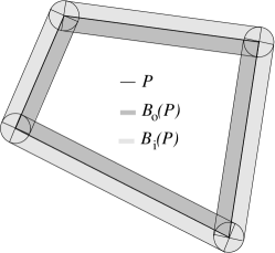
(a) The area of outside and inside strips.

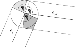
(b) Overlap between adjacent strips.

Figure 4: Geometry of boundary strips.

Theorem 6.1

Let $P$ be a simple closed polygonal curve with feature size at least $2R$ and total Euclidean length $\ell(P)$, consisting of edges $e_{i}$, and let $\varphi_{i}$ be the (outside) angle between edges $e_{i}$ and $e_{i+1}$. Let $B_{i}(P)$ be the set of all points that are near $P$ as an inner boundary, i.e., that are outside of $P$ and within distance $R$ of $P$, and let $B_{o}(P)$ be the set of all points that are near $P$ as an outside boundary, i.e., that are inside of $P$ and within distance $R$ of $P$. Then the area of $B_{o}(P)$ is $R\ell(P)-\sum_{\varphi_{i}>0}R^{2}\frac{\varphi_{i}}{2}+\sum_{\varphi_{i}<0}R^{2}\tan(\frac{-\varphi_{i}}{2})\pi R^{2}$, while the area of $B_{i}(P)$ is $R\ell(P)+\sum_{\varphi_{i}<0}R^{2}\frac{\varphi_{i}}{2}-\sum_{\varphi_{i}>0}R^{2}\tan(\frac{-\varphi_{i}}{2})\pi R^{2}$.

Proof

As shown in Figure 4, both $B_{o}(P)$ and $B_{i}(P)$ can be subdivided into a number of strips $s_{i}$ parallel to edges $e_{i}$ of $P$, and circular segments near vertices of $P$ that are either positive (when the angle between adjacent strips is positive, meaning there is a gap between the strips) or negative (when the angle is negative, meaning that strips overlap.) More precisely, if the angle $\varphi_{i}$ between edges $e_{i}$ and $e_{i+1}$ is positive, we get an additional area of $R^{2}\frac{\varphi_{i}}{2}$, while for a negative $\varphi_{i}$, the overlap is $R^{2}\tan(\frac{\varphi_{i}}{2})$. In total, this yields the claimed area. Our assumption on feature size guarantees that no further overlap occurs. ∎

Note that in any case, $\sum_{i}{\varphi_{i}}=2\pi$. Making use of this property is possible in various ways: It is natural to assume that the area for the exterior boundary strip is less than suggested by its length, while it should be larger for all other boundaries. This remains true for other kinds of boundary curves using similar arguments.

A straightforward estimate for strip area is given by the number $|N(D_{j})|$, while $|D_{j}|$ is a natural estimate for the length of the boundary, as the density of boundary nodes should be reasonably uniform along the boundary. Near boundary corners, the actual number of boundary nodes will be higher for convex corners (as the threshold of neighborhood size remains valid at larger distance from the boundary), and lower for nonconvex corners. Thus it makes sense to consider the ratio $\frac{|N(D_{j})|}{|D_{j}|}$ for all boundary components, as the outside boundary can be expected to have lower than average $|N(D_{j})|$ and higher than average $|D_{j}|$. The component with the lowest such ratio is the most likely candidate for being the outside boundary. See Table 1 for the values of our standard example.

	$D_{1}$	$D_{2}$	$D_{3}$	$D_{4}$
	(Outside boundary)	(Left eye)	(Right eye)	(Mouth)
$|N(D_{j})|$	6093	1304	1319	2368
$|D_{j}|$	2169	289	266	616
$\frac{|N(D_{j})|}{|D_{j}|}$	2.809	4.512	4.959	3.844

Table 1: Number of boundary nodes and near-boundary nodes for each boundary component.

The main appeal of this approach is that the required data is already available, so evaluation is extremely simple; we do not even have to determine hop count along the boundary.

It should be noted that our heuristic may produce wrong results if there is an extremely complicated inside boundary. This can be fixed by keeping track of angles (or curvature) along the boundary; however, the resulting protocols become more complicated, and we leave this extension to future work.

6.2 Using Boundary Distance

Once all boundaries have been determined, it is easy to compute boundary distances for each node by determining a hop count from the boundary. Note that this can be done to yield non-integral distances by assigning fractional distances to the near-boundary nodes, depending on their neighborhood size.

This makes it easy to compute the geometric thickness of the region: Compute a node with maximum boundary distance. In our standard example, this node is located between the three inside boundaries.

7 Experimental Results

All our above algorithms have been implemented and tested on different point sets. See the following Figure 5(a) for an example with 45,000 nodes and four boundaries. The bounding box has a size of $30R\times 30R$. Total area of the region is $786.9R^{2}$. Figure 5(b) shows the spatial distribution of neighborhood size. Notice the slope near the boundaries. Figure 6(a) shows the identified boundary, near-boundary and Voronoi nodes, shown as black dots, gray crosses, black triangles, while other interior nodes are drawn as thin gray dots. The total number of identified boundary or near-boundary nodes is 11,358, leaving 33,642 nodes as interior nodes. Finally, Figure 6(b) shows the assigned structural loops along the various boundary strips.

(a) Sensor network topology.

(b) Spatial distribution of $\left|N(v)\right|$.

Figure 5: Example network consisting of 45,000 nodes.

(a) Boundary nodes, near-boundary nodes, and Voronoi nodes.

(b) Structural loops along the boundaries.

Figure 6: Experimental results for the example network.

8 Conclusions

We have shown that dealing with topology issues in a large and dense sensor network is possible, even in the absence of location hardware or the computation of coordinates. We hope to continue this first study in various ways. One possible extension arises from recognizing more detailed Voronoi structures by making use of the shape of the boundary distance terrain: This shape differs for nodes that have only one closest line segment in the boundary, as opposed to nodes that are close to two different such segment, constituting a ridge in the terrain. Note that our Voronoi nodes are close to pieces from two different boundaries.

An obvious limitation of our present approach is the requirement for high density of nodes. A promising avenue for overcoming this deficiency is to exploit higher-order information of the neighborhood structure, using more sophisticated geometric properties and algorithms. This should also allow the discovery and construction of more complex aspects of the network, e.g., for routing and energy management.

References

- [AGY04] J. Aspnes, D. Goldenberg, and Y.R. Yang. On the computational complexity of sensor network localization. In Proc. ALGOSENSORS, 2004.
- [AR97] M.J.B. Appel and R.P. Russo. The maximum vertex degree of a graph on uniform points in . Adv. Applied Probability, 29:567–581, 1997.
- [Bea03] J. Beal. Near-optimal distributed failure circumscription. Technical Report AIM-2003-17, MIT Artificial Intelligence Laboratory, 2003.
- [BK98] H. Breu and D.G. Kirkpatrick. Unit disk graph recognition is NP-hard. Comp. Geom.: Theory Appl., 9(1-2):3–24, 1998.
- [BKKM96] J. Brunekreef, J.-P. Katoen, R. Koymans, and S. Mauw. Design and analysis of dynamic leader election protocols in broadcast networks. Distributed Computing, 9(4):157–171, 1996.
- [ČHH01] S. Čapkun, M. Hamdi, and J. Hubaux. GPS-free positioning in mobile ad-hoc networks. In Proc. IEEE HICSS-34—vol.9, page 9008, 2001.
- [DPG01] L. Doherty, K.S.J. Pister, and L. El Ghaoui. Convex position estimation in wireless sensor networks. In Proc. IEEE Infocom ’01, pages 1655–1663, 2001.
- [FGG04] Q. Fang, J. Gao, and L. J. Guibas. Locating and bypassing routing holes in sensor networks. In Proceedings IEEE Infocom ’04, 2004.
- [GHS83] R. G. Gallager, P. A. Humblet, and P. M. Spira. A distributed algorithm for minimum-weight spanning trees. ACM Transactions on Programming Languages and Systems, 5(1):66–77, 1983.
- [HT03] C.-F. Huang and Y.-C. Tsent. The coverage problem in a wireless sensor network. In Proc. ACM Int. WSNA, pages 115–121, 2003.
- [PBDT03] N.B. Priyantha, H. Balakrishnan, E. Demaine, and S. Teller. Anchor-free distributed localization in sensor networks. Technical Report MIT-LCS-TR-892, MIT Laboratory for Computer Science, APR 2003.
- [SB03] C. Stachniss and W. Burgard. Mapping and exploration with mobile robots using coverage maps. In Proc. IEEE/RSJ Int. Conf. IROS, 2003.
- [SR02] N. Sundaram and P. Ramanathan. Connectivity-based location estimation scheme for wireless ad hoc networks. In Proc. IEEE Globecom ’02, volume 1, pages 143–147, 2002.
- [SRL02] C. Savarese, J.M. Rabaey, and K. Langendoen. Robust positioning algorithms for distributed ad-hoc wireless sensor networks. In Proc. 2002 USENIX Ann. Tech. Conf., pages 317–327, 2002.