Single-Strip Triangulation of Manifolds with Arbitrary Topology

Abstract

Triangle strips have been widely used for efficient rendering. It is NP-complete to test whether a given triangulated model can be represented as a single triangle strip, so many heuristics have been proposed to partition models into few long strips. In this paper, we present a new algorithm for creating a single triangle loop or strip from a triangulated model. Our method applies a dual graph matching algorithm to partition the mesh into cycles, and then merges pairs of cycles by splitting adjacent triangles when necessary. New vertices are introduced at midpoints of edges and the new triangles thus formed are coplanar with their parent triangles, hence the visual fidelity of the geometry is not changed. We prove that the increase in the number of triangles due to this splitting is 50% in the worst case, however for all models we tested the increase was less than 2%. We also prove tight bounds on the number of triangles needed for a single-strip representation of a model with holes on its boundary. Our strips can be used not only for efficient rendering, but also for other applications including the generation of space filling curves on a manifold of any arbitrary topology.

1 Introduction

Constructing strips from an input set of triangles has been an active field of research in computer graphics and computational geometry, motivated by the need for efficient rendering in the former and by traveling salesman and Hamiltonian path problems in the latter. Traditionally, triangle stripification research has been pursued along two extreme problem statements. At one end, the input model is considered unchangeable and algorithms are designed to test whether there is a Hamiltonian path in the triangulation or to find as few strips as possible from the model. At the other end, the input triangulation is completely ignored, and a new triangulation is imposed on the input vertices in order to arrive at a single strip triangulation even if it requires addition of new vertices. The work presented here attempts to bridge the gap by finding a single strip triangulation from the input triangulation by splitting the input triangles if necessary while guaranteeing that the geometry of the input model is also retained.

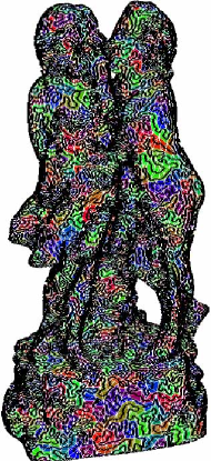
Figure 1: Single cycle triangulation of the genus-two sculpture model with 50780 input and 51780 output triangles.

Our motivation goes beyond the rendering requirement and theoretical aspects of Hamiltonian paths. The advantages of having a single triangle strip representation of a model enables a plethora of other geometric and topological algorithms to be applied on the model. In this paper, we show one such application – generating space filling curves on manifolds of arbitrary topology – using the total linear ordering of triangles given by a Hamiltonian cycle.

Triangle stripification algorithms can be categorized based on their input requirements. The first category of algorithms takes only the vertices of the model as input and finds a triangulation that would generate a single strip. The second category takes edges of a polygon as input and triangulates the interior of the polygon, with or without the addition of Steiner vertices, to create triangle strip(s) that covers the polygon. Typically, these two categories work only with data sets on a plane or a height field. The third category takes triangles of the model as input and tries to build long triangle strips, not necessarily a single strip, only using the input set of triangles. The third category works with 2D surfaces embedded in 3D. The algorithm presented in this paper is a combination of all the above three categories and creates a single triangle strip from the model. In the triangle strip generated by our method, all input vertices are used as in the first category, Steiner vertices and hence more triangles are added as in the second category, and finally, the geometry of the input triangulation is retained as in the third category.

1.1 Related Work

It follows from Steinitz’ theorem and known results on NP-completeness of the Hamiltonian cycle problem for cubic 3-connected planar graphs [GJT76] that it is NP-hard to find a single strip, even for a model consisting of a triangulated convex polyhedron, and known exponential-time algorithms for Hamiltonian cycles are not sufficient to find single strips for models of more than 100 triangles [Epp03]. Therefore, many algorithms simply attempt to find as few a strips as possible from the input triangulation. SGI developed a program [AHB90] that produces generalized triangle strips using a heuristic that begins and ends strips on faces with few neighbors, so as to reduce the number of isolated triangles. The classic STRIPE algorithm [ESV96] makes a global analysis of the input triangle mesh, trying to find patches that can be efficiently striped. Velho et al. [VdFG99] build and maintain triangle strips incrementally while creating a triangle mesh simultaneously. Chow [Cho97] builds strips by reusing the points added to previous strips as often as possible. Snoeyink and Speckmann [SS97] propose a stripification algorithm specially designed for triangulated irregular network (TIN) models using the spanning trees of the dual graphs of TIN models. Xiang et al. [XHM99] decompose spanning trees of the dual graph into triangle strips. The tunneling method for triangle strips in continuous level of detail meshes is proposed by Stewart [Ste01]. Taking this a step further, Shafae and Pajarola [SP03] propose dynamic triangle strip management for view-dependent mesh simplification and rendering algorithms. Demaine et al. [DEE^∗03] relaxed the definition of a triangle strip, to allow adjacent triangles in the strip to share only a single vertex instead of an edge, and showed that any model consisting of triangles meeting edge-to-edge (possibly with boundary) admits such a relaxed strip. Bogomjakov and Gotsman [BG02] investigate the ordering of triangles in order to reduce the number of vertex cache misses and develop methods to find triangle sequences that preserves the property of locality. Triangle strips are also important in geometric compression and transmission and is a by-product of these algorithms [Ros99, TG98]. Here again, the input triangulation is usually not modified.

The hardness of finding Hamiltonian paths can be eased by minor variations of the problem statement. For example, algorithms presented in [AHMS96] avoid Delaunay triangulation of the planar point set and create a Hamiltonian path triangulation. Further, they take as input a planar simple polygon, and check using its visibility graph whether there exists a single strip triangulation of the polygon’s interior. If not, such a triangulation is produced using Steiner vertices. They also prove that computing a Hamiltonian triangulation for planar polygons with holes is NP-hard. The QuadTIN method [PAL02] triangulates an irregular terrain point data set by adding Steiner vertices at quad-tree corners to produce a dynamic view-dependent triangulation that can be traversed as a single strip. Given a quadrilateral mesh of a manifold, Taubin [Tau02] splits each quadrilateral into triangles and orders them into a single strip. Unlike the above methods that take a quadrangulation or points on a plane or a height field as input, our method uses the triangulation of manifolds of arbitrary topology. Further, even by adding new triangles, our algorithm does not change the input geometry (in terms of visual fidelity), whereas the above methods prescribe a completely new triangulation that includes the input point set.

1.2 New Results

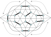
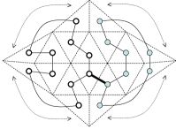
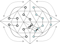
Figure 2: (a) The given triangulation. Assume that the boundary edges are adjacent to each other as shown by dotted arrows and all the boundary triangles share a common vertex. The mesh shown is a manifold with genus 0. (b) The dual degree three graph and a perfect matching shown by dark edges. (c) If we remove all the matched edges we get disjoint cycles consisting of only unmatched edges. Two such cycles, one with unfilled and the other with filled graph nodes are shown. The union of these cycles cover all the given vertices in the dual graph and hence the triangles in the given mesh. These disjoint cycles are connected to each other by matched edges. We construct a spanning tree of these disjoint cycles and hence choose matched edges that connect these cycles. (d) The triangle pair corresponding to chosen matched edges in the tree are split creating two new triangles. Matching is toggled around the new vertices resulting in a triangulation with a Hamiltonian cycle of unmatched edges as shown in the figure.

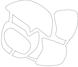
Figure 3: (a) An example of a graph of disjoint cycles of unmatched edges. These cycles are connected to each other by matched edges. (b) A spanning tree of cycles is constructed using selected matched edges. (c) These matched edges are split to create a Hamiltonian cycle.

Our main result is a new method for subdividing a triangulated model and finding a single triangle strip in the subdivided model. We show theoretically that this method is guaranteed not to increase the number of triangles in the model by more than 50%, but in our experiments the increase was at most 2%. In order to estimate how tight our worst case bounds are, we also construct a lower bound, consisting of an infinite family of triangulated models in which any method for subdividing the model to produce a single triangle strip must increase the number of triangles by at least 5.4%.

We also consider the problem of producing a single strip by subdividing a model having a triangulated boundary with holes. For such a model, with $n$ triangles, we show a tight bound of $3n-4\log_{2}n\pm O(1)$ on the number of triangles in the resulting strip. Therefore, starting with a watertight model is of considerable benefit in stripification.

2 Hamiltonian Cycle Stripification

In this section we describe our algorithm to create a Hamiltonian cycle from the given triangulation. The fundamental technique we use to arrive at a Hamiltonian cycle is a perfect matching algorithm. A matching in a graph $G=(V,E)$ is a subset M of the edges E such that no two edges in M share a common end node. A perfect matching $M$ in $G$ is a matching such that each node of $G$ is incident to an edge in $M$. (See Figure 2(b).) For a bridgeless graph in which every vertex has degree three, there always exists a perfect matching [Pet91]. Such a matching can be found in time $O(n)$ for planar graphs [BBDL01] or $O(n\log^{4}n)$ in general, where $n$ is the number of input vertices; the latter bound can be further improved to $O(n\log^{3}n\log\log n)$ using recent results of Thorup [Tho00]. In our case, we are interested in the dual graphs of triangulated manifolds; such graphs are bridgeless (in fact, 3-connected) and have degree three. A perfect matching in this dual graph will pair every triangle with exactly one of its adjacent triangles.

Given a perfect matching for a degree three graph, there are two unmatched edges incident on every graph vertex. The set of all unmatched edges forms a collection of disjoint cycles, the union of which covers the complete vertex set of the graph (Figure 2). These disjoint cycles are adjacent to each other across matched edges. Let us construct a graph called the cycle graph in which the nodes correspond to the disjoint cycles of this collection, and two nodes share an edge whenever the corresponding two cycles are adjacent to each other across a matched edge. From the cycle-graph, we construct a spanning tree of cycles (Figure 3). Considering this graph as the dual of our triangulation, the disjoint cycles are triangle strips (loops) and the matched edges in the tree are adjacent triangle pairs. As shown in Figures 2(d) and 3(c), we split each of these matched triangle pairs corresponding to the matched edges in the tree, to form a single cycle connecting all the triangles in the manifold.

If $k$ is the number of disjoint cycles then we need $(k-1)$ matched edges to form a spanning tree (Figure 3). Triangle pairs corresponding to these $(k-1)$ matched edges have to be split introducing $2(k-1)$ new triangles. Since the number of triangles in each cycle cannot be less than three, $k\leq\frac{n}{3}$. This worst case scenario results in $n+2\frac{n}{3}=1.66n$ triangles in the Hamiltonian cycle.

2.1 Eliminating Three-Cycles

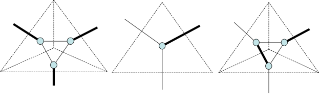
Figure 4: (a) A configuration of three triangles surrounding a degree-three vertex. (b) From the input mesh, all degree-three vertices are removed before finding the matching. The typical result after the matching is shown here. (c) The removed triangles are reinserted with appropriate matching between them. This local change does not change the matching outside the configuration. This process results in a perfect matching such that the unmatched edges have no three-cycles.

As discussed above, the worst case for our algorithm arises when the cycles of unmatched edges have length exactly three. We eliminate the possibility of occurrence of such three-cycles, improving our worst-case guarantees on the number of subdivisions, using the following observation. Cycles consisting of three triangles are formed only if there exists a configuration of three mutually adjacent triangles surrounding a degree-three vertex as shown in Figure 4(a). We temporarily simplify the mesh by repeatedly removing the central vertex from each such configuration, replacing the configuration by a single triangle (Figure 4(b)); in the dual graph of the mesh, this corresponds to a $\Delta$-$Y$ transformation in which a three-cycle is contracted to a single point. It is not a concern that this simplification may lead to self-intersecting geometry in the mesh. We can test whether any triangle belongs to a three-cycle by examining a constant number of nearby triangles, so the total time for this transformation is linear.

Once all three-cycles are removed, we then apply Petersen’s theorem to find a perfect matching in the simplified mesh. A typical result after such a matching is shown in Figure 4(b). We then add the removed three-triangle configurations back one at a time into this ‘matched’ mesh as shown in Figure 4(c). At each step, two of the triangles in the configuration are matched to each other, so that globally we retain a perfect matching with no three-cycles among the unmatched edges.

By means of this optimization, we are able to prove the following result.

Theorem 2.1

For any triangulated model with $n$ triangles, we can find in time $O(n\log^{3}n\log\log n)$ a subdivision of the model, and a single triangle strip for the subdivision, in which the subdivision has fewer than $3n/2$ triangles. If the model has the topology of the sphere then the time for finding a single strip subdivision can be further improved to $O(n)$.

Proof

As discussed above, we find a perfect matching in the dual of the input model, such that the unmatched edges form cycles with no three-cycle. Therefore, there can be at most $n/4$ cycles, $n/4-1$ edges selected in the spanning tree of the cycle graph, and $2(n/4-1)$ subdivisions. The total number of triangles is thus at most $3n/2-2$. The processes of removing and restoring three-triangle configurations, and of finding a spanning tree for the cycle graph and using it to select a set of subdivisions to perform, all take only linear time, so the total time is bounded by the algorithm for finding perfect matchings.

Although this worst case upper bound on additional number of triangles is 50% of the input number of triangles, in practice additional triangles is less than 2%. We achieve this result after using the further optimization described below. The results on lower bounds on additional triangles for both manifolds and manifolds with boundaries are given in the Appendix.

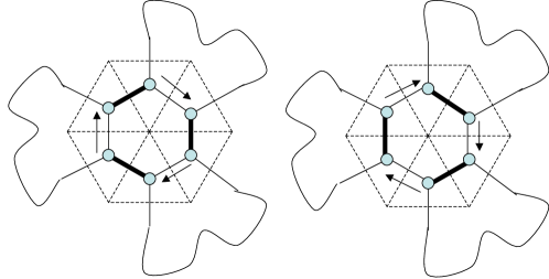
Figure 5: (a) A nodal vertex with (six) even number of incident triangles and triangles belonging to three unique cycles. (b) By switching the matched and unmatched edges, all these cycles can be merged to a single cycle.

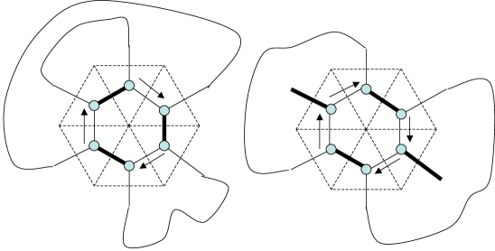
Figure 6: Examples of non-nodal vertices. In both the examples, there are six incident triangles but only two unique cycles.

2.2 Merging Cycles Around Nodal Vertices

The goal of this optimization is to increase the length of the disjoint cycles by merging many cycles without any triangle splits. Assume that we have already constructed a perfect matching, and partitioned the triangles of the input mesh into disjoint cycles. We classify a mesh vertex $v$ as a nodal vertex if it satisfies the following conditions: $v_{n}$, the number of triangles incident on $v$ is even and the total number of unique disjoint cycles that these incident triangles belong to is $\frac{v_{n}}{2}$. An example of a nodal vertex with six incident triangles and three unique incident cycles is shown in Figure 5. The neighborhood of every nodal vertex is modified such that the matched and unmatched triangle pairs are toggled. This merges all the incident cycles into one cycle. Examples of non-nodal vertices are shown in Figure 6.

If we use a union-find data structure to keep track of which triangles belong to which cycles, we can test whether any mesh vertex is nodal using a number of union-find queries proportional to the degree of the vertex, so the total time for the optimization is $O(n\alpha(n))$ where $\alpha$ is the extremely slowly growing inverse Ackermann function.

Once this optimization is performed, we form the cycle graph of the remaining cycles, construct a spanning tree, and use the tree to guide triangle subdivisions as before. This optimization step typically significantly reduces the number of subdivisions that must be performed, but we have no theoretical guarantees on its performance. The results of these optimizations on various models are shown in Table 1.

Model	Input Tris	Output Tris	% Increase
Torus	400	406	1.5
Sphere	480	484	0.8
Goblet	1000	1016	1.6
Eight	1536	1554	1.1
Sculpture	50780	51780	1.9
Fandisk	12946	13134	1.4
Horse	96966	98552	1.6
Shoe	156474	158980	1.6

Table 1: Results of our algorithm on different models. Note that the increase in number of triangles is consistently less than 2% of the input number of triangles.

3 Matching Implementation Details

We describe the implementation details only for the perfect matching phase of our algorithm, since the other parts of the algorithm are straightforward.

Rather than using the theoretically efficient but somewhat complex $O(n\log^{3}n\log\log n)$ algorithm to construct perfect matchings in the dual graphs of our models, we used a general purpose graph maximum matching algorithm, Edmonds’ blossom-contraction algorithm [Edm65]. This algorithm repeatedly increases the size of a matching by one edge, each time performing a breadth-first search using a union-find data structure to keep track of certain contracted subgraphs called blossoms. Therefore, if the number of repetitions is $k$, the total time is $O(kn\alpha(n))$.

In our application of this matching algorithm, the number of edges in the resulting matchings is always exactly $n/2$, so if we applied Edmonds’ algorithm starting from an empty matching we would take more than quadratic time, imposing strong limits on the size of the models we could handle. To reduce this time penalty, we precede Edmonds’ algorithm by a greedy matching phase, using the degree-one reductions and degree-two reductions described by Karp and Sipser [KS81] and Magun [Mag98]. This greedy matching phase typically matches 99.9% of the triangles of our input models, significantly reducing the time requirements for our perfect matching algorithm.

Our implementation of the matching portion of our strip finding algorithm is written in Python, a relatively slow interpreted language. On an 800 MHz Apple PowerBook, our code took approximately three minutes to find a perfect matching for the 90K-triangle horse model and took approximately seven minutes to find a perfect matching for the 150K shoe model. We expect that significant additional speedups could be obtained by rewriting our code in a faster compiled language, and by incorporating the more sophisticated greedy matching heuristics described by Magun [Mag98].

4 Applications

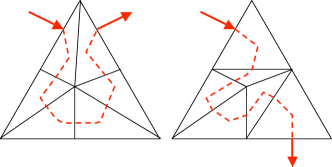
Figure 7: Depending on the direction of the cycle, two ways of subdividing a triangle are shown. Triangle vertices are assumed to be ordered in counter-clockwise direction. The space curve will pass through the edge centers and centroids of the triangles as shown. Recursive subdivisions would yield denser curves and eventually would fill the space of the given triangle.

Hamiltonian strip triangulation has many applications in rendering. One such application we elaborate here is a procedural method to generate space filling curves [Sag94] on the manifolds. Space filling curves are ideal for hierarchical indexing of a higher dimensional space with a single parameter curve. They have tremendous applications in many fields and are used to solve various problems on 2D images including contact searching [DHL^∗00], parallelizing finite element grid generation [BZ00], out-of-core visualization algorithms for massive mesh simplification [LP02] and volume rendering[PF01], mesh indexing [NS96], image compression [PW00], dithering [BV95], half-toning [ZW93], etc. Interesting applications of space filling curves in designing geometric data structures are detailed in [ARR^∗97]. Popular space filling curves include Hilbert curves and Lebesgue’s curves. A method proposed by Bartholdi and Goldsman [BG01] proposes a space filling curve on a vertex connected triangulation. Here we introduce a space filling curve that fills any (edge connected) triangulated manifold of any arbitrary topology. We believe that this procedural method to fill the surface with a single space-filling curve would enable researchers to do many of the geometric operations listed above, directly on the surface of 3D objects.

Since the cycle produced by our triangle strip method covers the whole model, a curve passing through the triangles of the strip, in order, would cover the whole model. If this curve fills each triangle on its way, it fills the space of any 2-manifold. Like any other space filling curve, we define our curve by recursive subdivision of the triangle. The subdivision should ensure that the new vertices converge to the vertices and centroid of the triangle. Hence edges have to be split by the subdivision. To ensure consistent subdivision of all the triangles and continuity of the curve across triangle boundaries, we impose a direction to the Hamiltonian cycle and also orient the manifold. Based on this direction of the cycle and the orientation of a triangle, we define two cases of subdivisions of the triangle, as shown in Figure 7. For any given point on the manifold’s surface, each level of subdivision reduces the diameter of the triangle containing that point by a constant factor, so the subdivision process produces in the limit a curve that passes arbitrarily close to the point and is therefore truly space-filling curve. Results of subdivision and space filling curves over multiple iterations are shown in Figures 8. As far as we know, this is the first procedural method to produce space filling curves on manifolds of arbitrary topology.

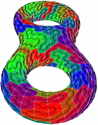
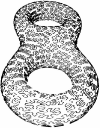
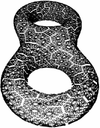
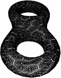
Figure 8: A double torus with multiple iterations of space filling curves.

5 Conclusion

We have presented a new algorithm to strip the given triangulation of a manifold into a single cycle covering all the input triangles. In the process we split a small number of pairs of adjacent triangles at the midpoint of their common edges. This addition of triangles will maintain the geometric visual fidelity of the original model. We have proven theoretical bounds on the output size of this algorithm, and also shown experimentally that in practice the algorithm performs much better than the theoretical bounds would suggest. We also presented one of the many applications of Hamiltonian cycle triangulation, namely, generating space filling curves on 2-manifolds with arbitrary topology.

There are many future directions to this project. In this current project, we have not considered the swap operations used in triangle strip rendering. New perfect matching algorithms that would take these constraints into account have to be developed. Total linear ordering of triangles is another powerful tool, but the Hamiltonian cycle provided by our algorithm is more than a total linear ordering, so perhaps some reduction in output size can be achieved by finding a path instead of a cycle. We believe that the existence of, and a procedural method to generate, a Hamiltonian cycle triangulation will spark varied interests in the research community.

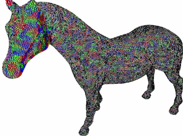
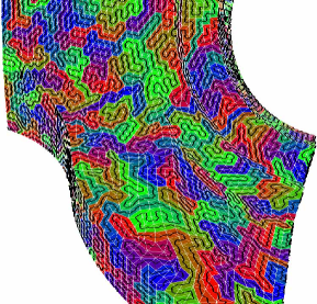
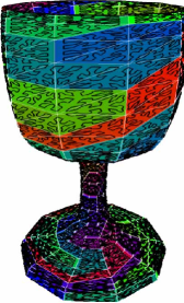
Figure 9: Horse model with 96966 input and 98552 output triangles. Fandisk model with 12946 input and 13134 triangles. Goblet with 1000 input and 1016 output triangles shown here with two iterations of space filling curve.

APPENDIX: Lower Bound Analysis

Although we proved a worst case bound of 50% on the increase in the number of triangles of a model due to our subdivision process, our experimental results show that increases of only 2% are more typical, and indicate to us that it may be possible to significantly improve our worst case bound. How much improvement is possible? To test this, we provide here a lower bound, showing the existence of models in which no subdivision method for producing single triangle strips can be guaranteed to achieve better than a 5.4% increase in the number of triangles.

Lower Bounds for Manifolds

The starting point of our lower bound is a result of Holton and McKay [HM88], that there exist non-Hamiltonian 3-connected 3-regular planar graphs with 38 vertices. The dual of such a graph is a mesh of 38 triangles that can be realized as a convex polyhedron and that has no cyclic strip of triangles. By connecting many such meshes together, we form a more general lower bound.

Theorem 5.1

There exists an infinite family of triangulated convex polyhedra, such that any single triangle strip formed by subdividing an $n$-triangle polyhedron in the family must have at least $39n/37-4$ triangles in the strip.

Proof

Let $H$ be the planar dual of the Holton-McKay graph; $H$ is a planar 3-connected graph with 38 triangular faces. For any $k$, let $A_{k}$ be any planar 3-connected graph with $k$ faces, all of which are triangles, and form a graph $G_{k}$ by replacing each triangle of $A_{k}$ by a copy of $H$. $G_{k}$ is thus a planar 3-connected graph with $n=37k$ faces, all of which are again triangles, so it can be realized as a convex polyhedron with triangle faces. The family described by the theorem consists of one such polyhedron for each $G_{k}$.

Now consider any single triangle strip formed by subdividing triangles of $G_{k}$. With the exception of at most two copies of $H$ (the copies containing the start and end of the strip) the remaining $k-2$ copies of $H$ must either be entered and exited exactly once by the strip (and therefore contain a subdivided edge in the interior of the copy, since $H$ has no cyclic triangle strip) or be entered and exited more than once (and therefore contain two subdivided edges on the triangle that was replaced by a copy of $H$). Thus, the total number of subdivided edges in the strip for $G_{n}$ is at least $k-2$. Each subdivided edge increases the number of triangles in the strip by two, so the total number of triangles in the strip is at least $39k-4=39n/37-4$.

Lower Bounds for Manifolds with Boundaries

Although our main results concern watertight models, we consider briefly for completeness the case of models with incomplete boundaries; we refer to any break in the boundary of a model as a hole.

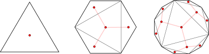
Figure 10: Recursive triangulations of regular $(3\cdot 2^{k})$-gons, and their dual complete trees.

Theorem 5.2

There exists an infinite family of triangulated models, having the topology of a sphere with a single hole, such that any single triangle strip formed by subdividing an $n$-triangle model in the family must have at least $3n-4\log_{2}n-O(1)$ triangles.

Proof

Form model $M_{k}$ by triangulating a regular $(3\cdot 2^{k})$-gon, so that there are $3\cdot 2^{k-1}$ outer triangles surrounding a central regular $(3\cdot 2^{k})$-gon, which is triangulated recursively to form a copy of $M_{k-1}$. As a base case for the recursion, let $M_{0}$ be a single equilateral triangle. Figure 10 depicts the first three models $M_{0}$, $M_{1}$, and $M_{2}$ in this sequence. As shown in the figure, the dual graph of $M_{k}$ is a tree with $n_{k}=3(2^{k}-1)+1$ nodes, corresponding to the same number of triangles in the model $M_{k}$. The longest path in this tree has length $2k$.

Now, consider any single triangle strip formed by subdividing $M_{k}$. Any interior edge of $M_{k}$ that is not along the path from the start triangle to the end triangle of the strip must be crossed an even number of times by the strip, so all but $2k$ of the edges are subdivided and the total number of subdivided edges is at least $n_{k}-1-2k$. As in the previous theorem, each subdivision increases the number of triangles by two, so the total number of triangles in the strip must be at least $3n_{k}-2-4k=3n_{k}-4\log_{2}n_{k}-O(1)$.

Finally, we show that the bound of Theorem 5.2 is tight.

Theorem 5.3

Any connected $n$-triangle model with holes can be subdivided to form a triangle strip with $3n-4\log_{2}n+O(1)$ triangles in the strip.

Proof

(sketch) Let $T$ be any spanning tree of the dual graph of the model, and let $e$ be an edge in $T$ such that the two subtrees on each side of $e$ each have at least $n/3$ triangles in them; such an edge can be found by stepping from edge to edge towards the largest subtree until the condition is met. Then, the path $P$ formed by connecting the leaves farthest from $e$ in each subtree has at least $\log_{2}n/3+\log_{2}2n/3=2\log_{2}n-O(1)$ edges. Form a multigraph $M$ by doubling each edge of $T$ except for the edges in $P$. $M$ has even degree except at the endpoints of $P$, so it has an Euler path that starts and ends at the endpoints of $P$. If we add a new vertex at the midpoint of each internal edge of $T$ except for the edges in $P$, and subdivide each triangle of the model appropriately, this Euler tour can be transformed into a triangle strip. There are $n-2\log_{2}n+O(1)$ new vertices, so the total number of triangles in the strip is $3n-4\log_{2}n+O(1)$.

References

- [AHB90] Akeley K., Haeberli P., Burns D.: The tomesh.c Program. Tech. Rep. SGI Developer’s Toolbox CD, Silicon Graphics, 1990.
- [AHMS96] Arkin E., Held M., Mitchell J. S. B., Skiena S.: Hamiltonian triangulations for fast rendering. The Visual Computer 12, 9 (1996), 429–444.
- [ARR∗97] Asano T., Ranjan D., Roos T., Welzl E., Widmayer P.: Space filling curves and their use in the design of geometric data structures. Theoretical Computer Science 181 (1997), 3–15.
- [BBDL01] Biedl T. C., Bose P., Demaine E. D., Lubiw A.: Efficient algorithms for Petersen’s matching theorem. J. Algorithms 38 (2001), 110–134.
- [BG01] Bartholdi J., Goldsman P.: A continuous spatial index of a triangulated surface, Part I: Standard triangulations. Manuscript, 2001. Online at http://www.isye.gatech.edu/~jjb/mow/Bartholdi-Goldsman-I.pdf.
- [BG02] Bogomjakov A., Gotsman C.: Universal rendering sequences for transparent vertex caching of progressive meshes. Computer Graphics Forum 21, 2 (2002), 137–148.
- [BV95] Buchanan J. W., Verevka O.: Colour dithering using a space filling curve. Tech. Rep. TR95-04, University of Alberta, 1995.
- [BZ00] Behrens J., Zimmermann J.: Parallelizing an unstructured grid generator with a space- lling curve approach. In Euro-Par 2000, LNCS 1900 (2000), Springer, pp. 815–823.
- [Cho97] Chow M. M.: Optimized geometry compression for real-time rendering. In Proceedings IEEE Visualization 97 (1997), IEEE, Computer Society Press, pp. 347–354.
- [DEE∗03] Demaine E. D., Eppstein D., Erickson J. G., Hart G. W., O’Rourke J.: Vertex-unfoldings of simplicial manifolds. In Discrete Geometry: In honor of W. Kuperberg’s 60th birthday, Bezdek A., (Ed.), no. 253 in Pure and Applied Mathematics. Marcel Dekker, 2003, pp. 215–228.
- [DHL∗00] Diekmann R., Hungershöfer J., Lux M., Taenzer L., Wierum J.-M.: Using space filling curves for efficient contact searching. In Proc. IMACS (2000).
- [Edm65] Edmonds J.: Paths, trees, and flowers. Canad. J. Math. 17, 449–467 (1965).
- [Epp03] Eppstein D.: The traveling salesman problem for cubic graphs. In Proc. 8th Worksh. Algorithms and Data Structures (2003), Dehne F., Sack J.-R.,, Smid M., (Eds.), no. 2748 in Lecture Notes in Computer Science, Springer-Verlag, pp. 307–318.
- [ESV96] Evans F., Skiena S., Varshney A.: Optimizing triangle strips for fast rendering. In Proceedings IEEE Visualization 96 (1996), Computer Society Press, pp. 319–326.
- [GJT76] Garey M. R., Johnson D. S., Tarjan R. E.: The planar Hamiltonian circuit problem is NP-complete. SIAM J. Comput. 5, 4 (1976), 704–714.
- [HM88] Holton D. A., McKay B. D.: The smallest non-Hamiltonian 3-connected cubic planar graphs have 38 vertices. J. Combinatorial Theory, Ser. B 45 (1988), 305–319.
- [KS81] Karp R. M., Sipser M.: Maximum matchings in sparse random graphs. In Proc. 22nd Annu. IEEE Symp. on Foundations of Computer Science (1981), pp. 364–375.
- [LP02] Lindstrom P., Pascucci V.: Terrain simplification simplified: A general framework for view-depandent out-of-core visualization. IEEE Transactions on Visualization and Computer Graphics 8, 3 (2002), 239–254.
- [Mag98] Magun J.: Greedy matching algorithms, an experimental study. ACM J. Experimental Algorithmics 3, 6 (1998).
- [NS96] Niedermeier R., Sanders P.: On the Manhattan-distance between points on space-filling mesh-indexings. Tech. Rep. IB 18/96, Universit at Karlsruhe, Fakultat fur Informatik, 1996.
- [PAL02] Pajarola R., Antonijuan M., Lario R.: QuadTIN: Quadtree based triangulated irregular networks. In Proceedings IEEE Visualization 2002 (2002), Computer Society Press, pp. 395–402.
- [Pet91] Peterson J. P. C.: Die theorie der regularen graphs (The Theory of Regular Graphs). Acta Mathematica 15 (1891), 193–220.
- [PF01] Pascucci V., Frank R. J.: Global static indexing for real-time exploration of very large regular grids. In Proceedings of the 2001 ACM/IEEE conference on Supercomputing (CDROM) (2001), ACM Press, pp. 2–2.
- [PW00] Pajarola R., Widmayer P.: An image compression method for spatial search. IEEE Transactions on Image Processing 9, 3 (March 2000), 357–365.
- [Ros99] Rossignac J.: Edgebreaker: Compressing the incidence graph of triangle meshes. IEEE Transactions on Visualization and Computer Graphics 5, 1 (January-March 1999), 47–61.
- [Sag94] Sagan H.: Space-Filling Curves. Springer-Verlag, 1994.
- [SP03] Shafae M., Pajarola R.: DStrips: Dynamic triangle strips for real-time mesh simplification and rendering. In Proceedings Pacific Graphics 2003 (2003), IEEE, Computer Society Press, pp. 271–280.
- [SS97] Szeliski R., Shum H.-Y.: Creating full view panoramic image mosaics and environment maps. In Proceedings SIGGRAPH 97 (1997), ACM SIGGRAPH, pp. 251–258.
- [Ste01] Stewart A. J.: Tunneling for triangle strips in continuous level-of-detail meshes. In Proceedings Graphics Interface 01 (2001), pp. 91–100.
- [Tau02] Taubin G.: Constructing Hamiltonian triangle strips on quadrilateral meshes. In Int. Worksh. on Visualization and Mathematics (2002). Also IBM Research Tech. Rep. RC-22295.
- [TG98] Touma C., Gotsman C.: Triangle mesh compression. In Proceedings Graphics Interface 98 (1998), pp. 26–34.
- [Tho00] Thorup M.: Near-optimal fully-dynamic graph connectivity. In Proc. 32nd Annu. ACM Symp. on Theory of Computing (2000), pp. 343–350.
- [VdFG99] Velho L., de Figueiredo L. H., Gomes J.: Hierarchical generalized triangle strips. The Visual Computer 15, 1 (1999), 21–35.
- [XHM99] Xiang X., Held M., Mitchell J. S. B.: Fast and effective stripification of polygonal surface models. In Proceedings Symposium on Interactive 3D Graphics (1999), ACM Press, pp. 71–78.
- [ZW93] Zhang Y., Webber R. E.: Space diffusion: an improved parallel halftoning technique using space-filling curves. In Proceedings of the 20th annual conference on Computer graphics and interactive techniques (1993), ACM Press, pp. 305–312.