A New Computational Framework For 2D Shape-Enclosing Contours

Abstract

In this paper, a new framework for one-dimensional contour extraction from discrete two-dimensional data sets is presented. Contour extraction is important in many scientific fields such as digital image processing, computer vision, pattern recognition, etc. This novel framework includes (but is not limited to) algorithms for dilated contour extraction, contour displacement, shape skeleton extraction, contour continuation, shape feature based contour refinement and contour simplification. Many of the new techniques depend strongly on the application of a Delaunay tessellation. In order to demonstrate the versatility of this novel toolbox approach, the contour extraction techniques presented here are applied to scientific problems in material science, biology, handwritten letter recognition, astronomy and heavy ion physics.

Keywords: Contour, Isocontour, Edge, Unstructured Grid, Delaunay tesselation, Skeleton, Shape morphology, Material surface, Bacterial colony, Handwritten letter recognition, Constellation, Freeze-out hyper-surface

I Introduction

In two spatial dimensions, a lower-dimensional interface which partitions a two-dimensional (2D) space into separate subdomains with nonzero areas is called a contour. 2D spaces can be either continuous or discrete with respect to a field quantity, which is defined across that particular space. For example, a 2D gray-level image represents a discrete 2D space with respect to the field quantity gray-level. Its area, which is covered by the image, is broken into many regular 2D cells, i.e., pixels ($=$ picture elements); each pixel has a constant shade of gray.
Many papers REF01 –REF06 have been written on the extraction of one-dimensional (1D) contours from 2D image data. It is not trivial to define a contour for a discrete space. For example, one has to specify how the final contour should be supported. Some contour extraction algorithms yield contours which only connect the centers of edge pixels (cf., e.g., Ref. REF07 ; an edge pixel is a pixel which is considered to represent a part of the boundary of a certain region of interest within a given image). Others may allow for the usage of points that lie on the boundary between two pixels (cf., e.g., Ref. REF08 ). More complications may arise, if a resulting contour is not closed or if it encloses an area which equals zero (in the latter case, we call a contour degenerate). Furthermore, a contour may be self-intersecting and as a result it may enclose more than one of the 2D regions.
One has also to consider the level of information, which is provided for building contours. In some applications, a 2D image is preprocessed through image segmentation REF08 –REF10 , i.e., pixels are grouped together into so called blobs. Very often, a contour extraction method is subsequently applied to the generated image blobs. In other applications, a 2D image is preprocessed by an edge detector (cf., e.g., Ref. REF11 ), i.e., edge pixels are identified which are assumed to describe the transition of two different neighboring regions (note, that an edge pixel is a 2D object rather than a section of a 1D contour). A contour extraction method may then be applied to the resulting edge pixels. In particular, complications may arise, if the edge pixels provided by an edge detector form only partially connected chains, or if the transition region (given by the edge pixels) of two zones in a 2D image exceeds the width of more than one pixel.
Ref.s REF01 –REF10 demonstrate that many different image processing problems have resulted in many different approaches for building 1D contours from 2D image data. It is therefore the intent of this paper to provide a single computational framework for building 2D shape-enclosing contours from various different types of 2D discrete data sets. The considered data sets will include both, 2D gray-level images and 2D simulation grids, e.g., 1+1D (i.e., 1D space + 1D time) hydrodynamic simulation data. The framework presented here will handle many different 2D image processing problems with one and the same set of tools. In particular, this novel framework will provide solutions for the problems described above and for others which one may be faced with when extracting contours from discrete 2D data sets. Note, that the results of this framework will depend strongly on the quality of preprocessed data, e.g., the segmentation of 2D image data. The latter subject is beyond the scope of this paper. We will rather focus on some of the geometrical features of the properly preprocessed 2D data.
This paper is structured as follows. In the next section, the contour extraction framework is explained. The topics which are covered in this section include (but are not limited to) dilated contour extraction REF12 , contour displacement, shape skeleton extraction, gap closure or contour continuation, shape feature based contour refinement and contour simplification. This section is followed by an application section, where this novel toolbox approach for 1D contour extraction is applied to scientific problems in material science, biology, handwritten letter recognition, astronomy and heavy ion physics. A summary will conclude this paper.

II The Contour Extraction Framework

In this section, we decribe how to extract 1D contours from discrete 2D spaces. As mentioned above, a discrete 2D space could be represented by a 2D image. However, a proper discrete 2D space could also be given through the union of all triangles resulting from a 2D Delaunay tessellation REF13 (including some additional field quantities that characterize each triangle further), etc. REF02 . In the next section however, we shall restrict ourselves - without loss of generality - to the case of 2D images. Note, that the following contour extraction algorithm REF12 , which is also known under the name DICONEX, has been implemented efficiently into software REF14 .

II.1 DICONEX - DIlated CONtour EXtraction

The DICONEX algorithm REF15 –REF17 always yields perfect contours for both, binary and gray-level images. The contours are perfect in the sense that they are non-selfintersecting and non-degenerate, i.e., the contours always enclose an area larger than zero. DICONEX operates on a segmented 2D image (or comparable data structure). Fig. 1.a shows a binary image with 25 white and 11 gray pixels.
As a first step, a set of disconnected vectors is constructed which separates white pixels from gray ones. Each vector is attached to a pixel with its origin and its endpoint in such a way that the pixel always lies to the left of the vector (cf., Fig. 1.b). This ensures the counterclockwise circumscription of all pixels (or clusters of pixels) by the vectors. Conversely, all holes in a pixel cluster (blob) are circumscribed clockwise (cf., Fig. 1.c and Fig. 1.d). Note, that in order to accomplish this pixel enclosure by oriented vectors, it is only necessary to consider the four nearest neighbors of any given pixel, i.e., its upper, left, lower, and right pixel neighbor (cf., Fig. 1.b). Each vector is unique, double counting can never occur. Furthermore, there is no specific order required in which the neighborhood of any given pixel is evaluated. Therefore, this processing step is totally parallel.

Figure 1: (a) Initial binary image; (b) contour vectors for a single pixel; (c) left-turning and (d) right-turning contour vectors for initial binary image; (e) dilated contours for left-turning contour vectors (“disconnect” mode); (f) dilated contours for right-turning contour vectors (“connect” mode).

In the second step, which is linear, connected loops are constructed from the previously generated contour vector set. Each vector is attached with its origin to the end point of another vector. When connecting the vectors to contours, one starts with a single vector. Note, that each vector will contribute to the set of contructed contours only once. If one attaches the next vector, which has its origin attached to the end point of the current vector, one is always faced with either one of the two following options. Either there is one vector or there are more than one vectors (e.g., two in the case of pixel processing) connected to a single vector. In the latter case, the user has to decide, if a pixel should be disconnected or connected to the current blob whose enclosing contour is being constructed; we either choose always a left-turn (cf., Fig. 1.c) or always a right-turn (cf., Fig. 1.d,) when connecting the vectors. In doing so, we ensure a consistent choice for building the contours while tracing the sequence of vector origins. Additionally, we either weaken the connectivity between pixels which touch each other only in one point or we strengthen it. In fact, the dilated versions of the contours will lead either to a total separation (cf., Fig. 1.e) or to a merging (cf., Fig. 1.f) between two pixels that share only one common (pixel corner) point. Fig. 1.c and 1.d show the left-turn and right-turn contours, respectively, for the rendered bi-level (binary) image shown underneath.
Finally, the vector origins are replaced with the midpoints between the origins and the endpoints of the contour vectors without changing the connectivity among the vectors. As a result, one obtains modified contours which represent a dilation of the centers of the blob edge pixels. Figs. 1.e and 1.f depict the dilated contours according to the technique outlined here. Note, that in some of the following figures the arrow heads of the vectors will be omitted.

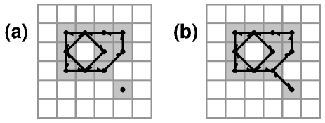
Figure 2: (a) boundary pixel tracing contours (“disconnect” mode); (b) boundary pixel tracing contours (“connect” mode).

II.2 Boundary pixel tracing contours

Another type of contour can be obtained by tracing the pixel boundary of image blobs REF07 while connecting the pixel centers. Such boundary pixel tracing contours (BPTCs) have the advantage that they can be obtained with very little memory requirement while making use of so called chain codes. A chain code is a sequence of directions, typically indicating the shortest path to one of the next eight neighbors of a given pixel. However, if holes are present within the shapes of a given pixel cluster, an algorithm may be unable to construct the contours successfully REF06 .
The DICONEX algorithm can also be used to construct BPTCs. Instead of finally replacing the origin of a contour vector with the midpoint between its origin and its endpoint, the origin of a contour vector is moved to the center of the pixel to which the contour vector is attached to initially. Fig. 2 shows BPTCs according to this technique.
Note, that there are two contour solutions possible for the pixel configuration shown in Fig. 2, because a pixel which is in contact with another one in only one point may be disconnected from or connected to its apparent partner. In fact, it is this ambiguity that may cause an algorithm to crash in its effort to construct BPTCs successfully, because it may not have accounted for such cases consistently. We would like to stress that the BPTCs may be self-intersecting and - partially or fully - degenerate (cf., e.g., the point in Fig. 2.a is a fully degenerate contour).

II.3 Isocontours

Sometimes, 2D gray-level image data are processed with the intent to extract isocontours. An isocontour is a contour which has a constant value at all of its supporting points with respect to the field quantity that has been used for the contour extraction. Because the points which support a DICONEX contour always coincide with the midpoints of the boundary edge between two pixels, dilated contours are in general not isocontours. However, these contours can be transformed into isocontours very easily.
Fig. 3.a shows a 2D gray-level image with 36 pixels. Here, black pixels have a gray-level of value zero, whereas white pixels have a gray-level of value 255. We shall now construct an isocontour corresponding to a gray-level of value 100. First, all pixels with a gray-level of value larger than or equal to 100 are enclosed with contour vectors as depicted in Fig. 3.b. From these contour vectors a dilated contour is constructed as shown in Fig. 3.c. In Fig. 3.c, additional vectors are drawn for each of the points that support the DICONEX contour. We will refer to these additional vectors as range vectors. Each range vector connects the centers of the pair of pixels that share the boundary edge of the initial contour vectors. The origin of a range vector coincides with the pixel center of the larger gray-level value, whereas its endpoint coincides with the pixel center of the smaller gray-level value.

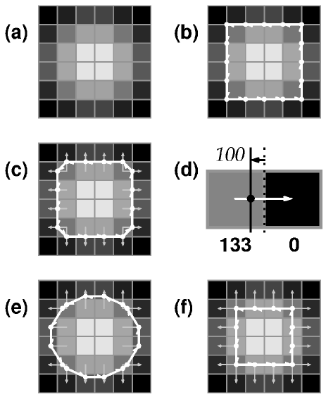
Figure 3: (a) Initial gray-level image; (b) as in (a), but with left-turning contour vectors; (c) as in (a), but with range vectors and dilated contour; (d) contour displacement for a pixel pair (see text); (e) gray-level image superimposed with range vectors and an isocontour of value 100; (f) as in (e), but with boundary pixel tracing contour.

Fig. 3.d illustrates how DICONEX contours can be transformed into isocontours. Two pixels - one with a gray-level value of 133, the other one with a zero valued gray-level - are initially separated by a DICONEX contour section that is located exactly in the middle between them (dotted line). A range vector connects the centers of the two pixels. It defines the bounds within which the support point for a dilated contour may be displaced. The centers of each pixel are assumed to correspond exactly with their gray-level values. The location of the support point for the isocontour is located closer to the center of the pixel with the gray-level of value 133. Note, that within this paper we use linear interpolation of the gray-levels. In Fig. 3.e, the dilated contour of Fig. 3.c has been transformed into an isocontour representing a gray-level of value 100.
While using range vectors, one may transform a dilated contour also into a boundary pixel tracing contour (cf., the previous section). One simply has to move all points which support a dilated contour to the origins of the corresponding range vectors as shown in Fig. 3.f.
Note, that the decision whether contours should be left- or right-turning can also be made locally when using gray-level images. Then one could consistenly use left-turns, if the turning point under consideration has an interpolated gray-level value above the isocontours gray-level value. Right-turns would then be taken otherwise, or vice versa.

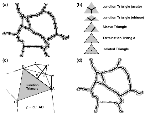
Figure 4: (a) A shape with internal triangle decomposition and skeleton; (b) triangles with shape skeleton segments (the dashed lines indicate segments of a shape contour); (c) geometric pruning for skeletons (see text); (d) as in (a), but with a pruned skeleton.

II.4 Delaunay tessellation and shape skeleton

Edge detection algorithms such as the Canny edge detector REF11 return when applied to a 2D gray-level image a set of 2D pixels rather than 1D contours or contour segments. Here, we prefer to generate 1D contours from a given set of edge pixels. In the following, a set of edge pixels will represent 2D shapes from which we are going to extract their skeletons in terms of 1D contours or at least contour segments.
First, we generate DICONEX contours for the edge pixel blobs. Next, the dilated contours and their supporting point set will be processed with a constrained Delaunay tessellation (CDT). Note, that no additional “Steiner” points REF13 will be added to this tesselation. In Fig. 4.a, the interior of a 2D shape is decomposed into a set of triangles after application of a CDT. This is the key step that allows for the skeleton extraction of the shape REF18 –REF20 . The triangles originating from the Delaunay tessellation can be classified into four types, namely those with three, two, one or none external (i.e., polygonal boundary) edges. Accordingly, we denote these triangles as “isolated,” “terminated” (T), “sleeve” (S), and “junction” (J) triangles, respectively. For each triangle, line segments or single points can be drawn (cf., Fig. 4.b), which in their union represent a skeleton of the processed shape.
Fig. 4.a shows in addition to the CDT of the 2D shape’s interior also its shape skeleton. Because of small variations along the shape’s enclosing contour, structurally unimportant skeleton features may occur. However, these can be removed according to the following pruning method REF19 . Initially, all junction triangles are evaluated based on their nesting level within a given shape. Junction triangles which are nested most deeply are processed first, those which are closest to the shapes contour(s) are processed last. Fig. 4.c provides an example for pruning. For a given junction triangle $ABC$, we consider its edge $AB$ and the shapes contour section $AopqrB$. For each point of the set $P=\{o,p,q,r\}$, we compute the distance $d$ to the junction triangle’s edge $AB$. Let $\rho\equiv d/|AB|$ be the ratio of morphological significance. If for any of the points in $P$, the ratio $\rho$ exceeds or equals a fixed threshold, $\rho_{0}$, the contour section and the corresponding skeleton branch will be preserved, otherwise closed polygon $AopqrBA$ will be removed. As a consequence, the junction triangle may turn into a sleeve triangle, where the triangle edge $AB$ becomes a new (virtual) shape boundary edge.
Note, that before the junction triangle is turned into a sleeve triangle, the above algorithm is also applied to the edges $BC$ and $CA$. Hence, a junction triangle could even turn into a terminal or into an isolated triangle. In Fig. 4.d, the pruned skeleton is shown for the inital 2D shape of Fig. 4.a with a threshold $\rho_{0}=0.6$.

II.5 Frame addition and gap closure

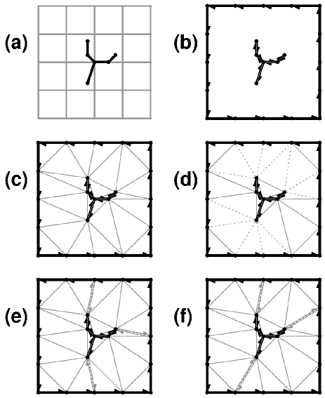
Figure 5: (a) A pixel frame superimposed with a shape skeleton; (b) shape skeleton vectors and frame vectors; (c) as in (b), but with additional Delaunay triangular mesh; (d) as in (c), but with suggested gap closure lines (dotted); (e) as in (c), but with gap closing vector pairs (gray) of shortest length; (f) as in (c), but with vector pairs (gray), which attempt to conserve directions.

Edge pixels are very often generated in order to decompose 2D image data into several disjunct regions. However, their shape skeletons may not always provide a complete partitioning of the underlying 2D space. In the following, we apply a frame addition and gap closure technique REF17 to an initially given skeleton in order to partition an image into several contour-enclosed non-zero areas.
In Fig. 5.a, an image area of 4x4 pixels is shown, which is superimposed by a shape skeleton. First, two opposite vectors are assigned to each line segment of the shape skeleton, so that the length and orientation of each vector pair coincides with the length and orientation of each of the skeleton’s line segments (cf., Fig. 5.b). Next, a frame of vectors is added around the original image given in Fig. 5.a. These outer frame vectors are arranged counterclockwise around the original image as shown in Fig. 5.b. The point set which supports the frame’s vector set is sampled at the rate of pixels available along a side of the image. In particular, it includes the four corners of the image.
In order to close the gaps between the skeleton and the frame, a CDT is applied to the point set, which supports the skeleton and the image frame (cf., Fig. 5.c). Certain edges (shown dotted in Fig. 5.d) of the unstructured grid connect the terminal points of the skeletons’ limb-like arcs with the outer image frame. Now, one could either select the shortest edges (cf., Fig. 5.e) or the edges which preserve mostly the orientation of the terminating vector pair in a skeletons’ limb (cf., Fig. 5.f) among the edges bridging a gap between a terminal point and a frame point. In either event, the gaps will then be closed with vector pairs of opposing direction. Finally, all vectors can be connected to region-enclosing contours exactly the same way as it is prescribed by the DICONEX algorithm (here, only left-turns will be performed whenever junctions are encountered). Note, that this gap closure technique can be easily extended to general gap closure or edge continuation between disjunct skeletons.

II.6 Contour refinement using shape features

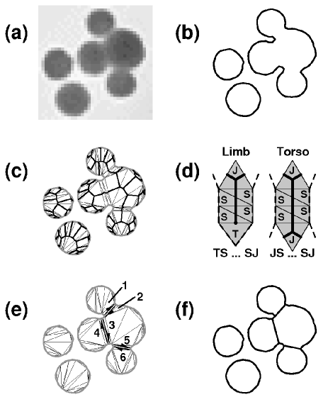
Figure 6: (a) Initial gray-level image; (b) three isocontours for the dark spots in image (a); (c) shape skeletons, which are enclosed by the contours in (b); (d) a limb and a torso (see text); (e) torso-splitting vector pairs (black); (f) six final shape-enclosing contours.

The contours which may be extracted from 2D image data very often do not resemble the shapes which a human observer might expect. For example, Fig. 6.a shows a gray-level image with six circular shaped dark pixel clusters, of which four of them slightly overlap. Isocontour extraction as described previously in this paper results in three shape-enclosing contours as shown in Fig. 6.b for an isovalue of 130. A human observer might have expected the extraction of six contours instead. In the following, we describe a technique REF21 which allows us to increase the initially found number of contours by three while making use of higher-level shape features.
In Fig. 6.c, the interiors of the three contours have been decomposed through a CDT and the unpruned shape skeletons are depicted. Ref.s REF18 –REF20 have made clear the value of Delaunay triangulations in obtaining structurally meaningful decompositions of shapes into simpler components. 2D shapes can be decomposed into generic shape components, the so called limbs and torsos REF18 ; REF19 . A “limb” is a chain complex of pairwise adjacent triangles which begins with a junction triangle and ends with a termination triangle. A “torso” is a chain complex of pairwise adjacent triangles, which both begins and ends with a junction triangle (cf., Fig. 6.d). Note, that a string-like shape, i.e., $TS...ST$, is a degenerate limb, whereas a torus-like shape, i.e., $S_{o}S_{1}...S_{N}S_{o}$, is a degenerate torso.
Here (cf., Fig. 6.e), the torsos play an important role which are encapsulated by the junction triangle pairs $1\&2$, $3\&4$, and $5\&6$. For these torsos only, none of the longest edges of both encapsulating junction triangles face their other junction triangle partner. If vector pairs are placed with opposing directions at the narrowest local widths for these torsos, we may break-up the considered contour into four. Note, that the initial shape-enclosing contours consist of vector sequences, which enclose the shapes counterclockwise. After insertion of the vector pairs, all vectors can be newly connected to region-enclosing contours as it is prescribed by the DICONEX algorithm (once again, only left-turns will be performed whenever junctions are encountered). Hence, we end up with four separate contours for the four overlapping circular shaped dark pixel clusters, whereas the other two contours remain unchanged (cf., Fig. 6.f).
Very often it is possible to reduce the number of points which support region-enclosing contours. For example, it is sufficient to represent contour sections which form straight lines by two points only. The same may apply for contour segments which turn only very little. For the down-sampling of contours various techniques REF22 –REF24 have been proposed. In this paper, we shall use a method (cf., Ref. REF17 ) which requires only local contour information when points are evaluated for removal.
This section concludes the theoretical part of the here presented framework.

III Applications

In this section, we demonstrate the versatility of the above described toolset for contour extraction, etc., by considering a rather diverse group of applications. First, we process an image generated by electron backscattered diffraction in order to better quantitatively describe a granular metal surface. In a second application, we are going to improve on the counting of bacterial colonies within a given image of a Petri dish. Thirdly, we process an image showing a handwritten Japanese letter in order to extract its structural shape features. Next, we treat an image which shows a distribution of stars. In a fifth and last application, we process 1+1D relativistic hydrodynamic simulation data in order to obtain a freeze-out hyper-surface for subatomic multi-particle production.

III.1 Region-enclosing contours for EBSD imagery

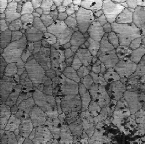
Figure 7: Backscattered contrast image REF27 of a thin Aluminum film.

The accurate characterization of the structures and properties of grain boundary networks is one of the fundamental problems in interface science. The Electron BackScattered Diffraction REF25 (EBSD) technique provides experimental results on grain boundary properties and grain growth in metal surfaces. In EBSD experiments, images of various material surfaces are recorded by secondary electron or backscattered contrast and corrected for instrumental distortions. For the extraction of the information contained in the images, it is important to locate the grain boundaries and triple junctions between grains. This localization task is accomplished by shape processing techniques, which have been presented in the previous sections. The resulting region-enclosing contour information is essential for mesh generation REF26 and the characterization of the morphology and topology of grain distributions.
In this section, we follow the processing of an experimental EBSD image with the above decribed shape processing algorithms. Fig. 7 shows an example of a backscattered contrast image REF27 of a thin Aluminum film with a columnar grain structure. Using an image which is recorded simultaneously from secondary electron emission, researchers are able to determine the grain edge pixels with rather standard REF08 –REF10 pixel processing techniques (cf., Ref.s REF25 ; REF26 ; e.g., in Ref. REF28 , grain boundary information is obtained from imagery taken by transmission electron microscopy).

Figure 8: Processing a sub-region of the resulting binary image: (a) dilated contours enclose the gray pixels; (b) shape skeleton and added outer frame; (c) CDT for the final closed contours (the closed gaps are drawn with larger line width); (d) gray pixels superimposed with down-sampled shape-enclosing contours and a CDT grid.

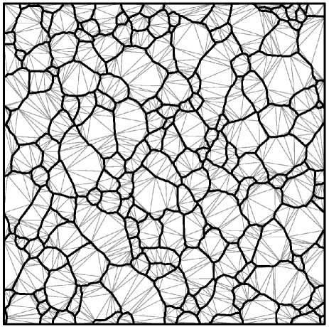
Figure 9: Shape-enclosing contours and a CDT grid for the binarized image of Fig. 7.

In the following, we shall restrict our discussion to a sub-region (cf., Fig. 8.a) of the resulting bi-level image of grain edge pixels without loss of generality. The goal is to process the given grain edge pixels in order to obtain as a final result a set of contours, where (i) each contour encloses a grain (region) counter-clockwise with a minimum number of supporting points according to the initially given edge pixels, and where (ii) the whole area of the image has been taken under consideration (cf., Fig. 8.d). This can be accomplished as follows.
First, right-turning, i.e., pixel connecting, DICONEX contours are generated for the gray pixels shown in Fig. 8.a. Then, a CDT is applied to the dilated contours and their supporting point set in order to decompose the interior of the shape into triangles. Using the individual morphological roles of the triangles, a pruned skeleton (with $\rho_{0}=0.6$) is generated (cf., Fig. 8.b). It encloses only three of the nine visible grains fully. Because it is our intent to construct region-enclosing contours for all nine visible grains, a frame (which also is shown in Fig. 8.b) is added around the original image area. A subsequent CDT is applied to the point set of the skeleton and of the image frame (cf., Fig. 8.c). For this current application, we choose to preserve the orientation of the last line segment for a limb-like skeleton arc as much as possible when connecting it to the frame (cf. Fig. 8.c). Considering the vector sets of (i) the shape skeleton, (ii) the image frame, and (iii) the gap vectors, we apply the above described contour element connection algorithm (cf., section 2.1) in order to connect all vectors into discrete region-enclosing contours (note, that only left-turns will be performed, whenever contour junctions are encountered). However, the region-enclosing contours are rather densely sampled. In Fig. 8.c, the contours are sampled with 599 points, and the Delaunay mesh shown here consists of 986 triangles. Therefore, we simplify the contours with the technique explained in Ref. REF17 (in particular, we have chosen $w_{0}=0.7$ of the pixel width, cf., Ref. REF17 ). In Fig. 8.d, the final contours are sampled with only 38 points, and the Delaunay mesh shown here consists of only 64 triangles. Note, that the region-enclosing contours stay within the limits defined by the gray pixels.
Full processing REF17 of the full binary image (not shown here) with 25,518 grain edge pixels leads to only 1,368 region-enclosing contour support points for 177 grain regions, and the accurate coverage of all grains requires only 2,678 Delaunay triangles (cf., Fig. 9).

III.2 Bacterial colony counting

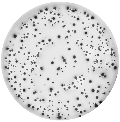
Figure 10: Gray-level image REF30 of the interior of a Petri dish with E. coli colonies.

In studies of the population dynamics of the intestinal population of mice, the most basic measure of how the population of a certain species is behaving is the abundance of the organisms REF29 . As such, fecal sampling and plating at several dilutions on selective media allows the biologist to get a measure of the abundance of organisms in the lower colon of mice. Counting colony forming units (CFUs) is a traditional way of measuring the population density of any bacterial culture or natural bacterial source. Fig. 10 shows the interior of a Petri dish with E. coli colonies, which have been recovered from the fecal pellets of mice REF30 . E. coli is the abbreviated name of the bacterium in the family Enterobacteriaceae named Escherichia coli.
In clinical studies, researchers usually take repeated samples for statistical reasons. Giving the mice under consideration various treatments which alter their intestinal flora results in different effects in the population densities. Even a small experiment with – let’s say – 36 mice, will produce hundreds of plates per sample point and can be sampled several times daily. The abundance of visual data makes the automation of visual bacterial colony counting highly desirable. However, the separation of overlapping colonies is a challenging task for standard image processing techniques, i.e., it is not trivial to provide the correct number of CFUs present in a given image. In total one obtains 415 isocontours (for an arbitrarily chosen isovalue of 130) for Fig. 10 when applying the contour extraction techniques outlined in sections 2.1 and 2.3, respectively. However, some of the contours then enclose more than a single CFU. Therefore, this number of 415 contours does not reflect the correct number of CFUs present in Fig. 10.
In section 2.6, it was explained how one can refine the contours, in order to decompose the enclosed shapes into a maximum of convex shaped constituents (cf., also Ref. REF21 ). In fact, Fig. 6.a is a subregion of the image in Fig. 10 at an increased resolution. In section 2.6, we were able to count all of the shown CFUs correctly. Fig. 11 shows the refined contours. Note, that the number of contours (and therefore the number of registrated CFUs) increases from 415 to 451 in Fig. 11. However, there are still quite a number of contours, which the reader possibly would have refined as well. The contour refinement technique as described in section 2.6 is very sensitive to the particular result of the constrained Delaunay tessellation. The CDT in return, is very dependent on the quality of the contours. Small variations in the contours can be caused, e.g., by noise in the image data. However, it is beyond the scope of this paper to address a proper treatment of noise (as well as other topics such as proper illumination of the sample, etc.) for the image data shown in Fig. 10. Hence, we conclude this section with the notion that we have obtained a significant improvement in our attempt to count bacterial colonies through our new framework for contour extraction.

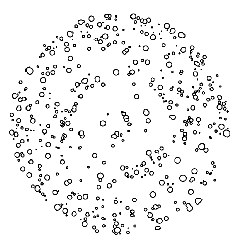
Figure 11: Shape-enclosing contours for the E. coli colonies in Fig. 10. after contour refinement (see text).

III.3 Towards handwritten letter recognition

Shape analysis and its classification is of great interest within the field of image processing (cf., e.g., also Ref. REF31 and Refs. therein). In section 2.4, a technique has been described which provides skeletons for contours that enclose pixel regions representing a certain shape. In fact, a shape skeleton can be viewed as a graphical representation REF32 ; REF33 of such an initially given shape (cf., also section 2.6). Refs. REF34 ; REF35 decribe, how a skeleton may be processed further so that more knowledge about its represented shape can be gained. In particular, such an approach allows for shape recognition. Its detailed description, however, is beyond the scope of this paper. Instead, we provide an example, which demonstrates the transformation of the image of a handwritten character into its graphical, i.e., skeletal representation.
In Fig. 12.a, a handwritten character, the Japanese Hiragana “A,” is depicted. All pixels which have a gray-level in the range from $0$ to $150$ have been selected and their union has been enclosed with dilated contours (cf., Fig. 12.b). In Fig. 12.c, a CDT has been applied to the point set which supports the contours. Here, we show both the interior and exterior triangles of the mesh. The distinction between interior and exterior triangles is rather straigthforward, since the dilated contours enclose shapes always counterclockwise, whereas holes of shapes are always enclosed clockwise.

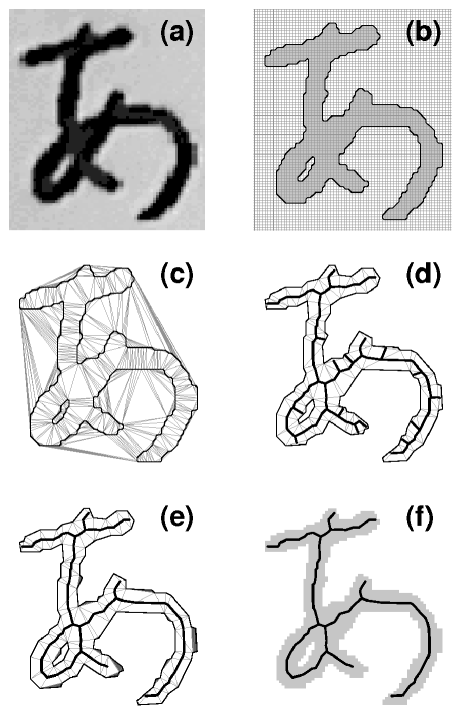
Figure 12: (a) A gray-level image resulting from the scan of a handwritten Japanese letter, the hiragana “A;” (b) dilated contours enclose the selected gray pixels; (c) CDT for the dilated contours; (d) CDT and skeleton segments for the interior of the shape, which is enclosed by down-sampled dilated contours; (e) as in (d), but with a pruned skeleton; (f) selected gray pixels superimposed with the pruned skeleton as shown in (e).

The here shown triangular CDT mesh consists of $526$ interior triangles; $93$ of them are junction triangles. This rather large number of junction triangles is mainly caused by the many directional changes in the contours. After down-sampling of the contours with the technique outlined in Ref. REF17 (again, we have chosen $w_{0}=0.7$ of the pixel width here), we obtain a much coarser CDT mesh. The result is shown in Fig. 12.d, where we have only $103$ interior triangles; this time, only $18$ of them are junction triangles. However, the shape’s skeleton still contains limbs which are of apparent lesser morphological significance.
Pruning of the shape with $\rho_{0}=0.4$ yields a skeleton which resembles its morphology quite well (cf., Fig. 12.e). The final number of junction triangles is $6$ out of $88$ unpruned triangles. In Fig. 12.f, the final shape skeleton is superimposed to the original selected pixels. Note, that the skeleton stays completely within the area defined by the pixels, which represent the handwritten character. We conclude this section by refering the more interested reader once again to Refs. REF34 ; REF35 , where the subsequent shape recognition processing steps are explained in great detail (for alternate pattern recognition methods,cf., e.g., Ref. REF36 and Refs. therein).

III.4 Stargazing

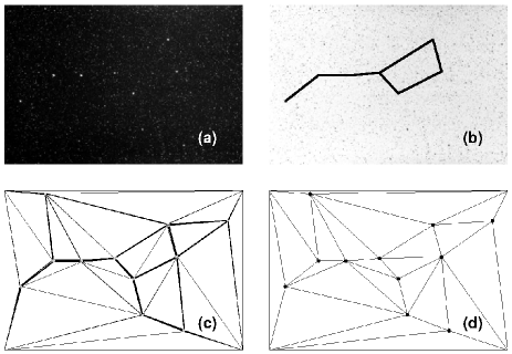
Figure 13: (a) A night sky scene of the northern hemisphere showing the Big Dipper (see text); (b) inverted gray-level image (a) with line segments connecting the stars of the Big Dipper; (c) CDT for the dilated contours of the pixels representing some of the brigthest stars plus the four corners of image (a); (d) CDT for the centers of gravity for the star shapes plus the four corners of image (a).

For ages, particularly bright stars of the starry sky have been combined into constellations REF37 . In the northern hemisphere, e.g., the Big Dipper – a group of seven bright stars (cf., Fig. 13.a) that dominate the constellation Ursa Major the Great Bear – can be observed in the night sky during any season. Apparently, it is the human eye which sometimes can makeup invisible lines, where there are actually none REF38 . That is why one tends to connect close stars with virtual lines, as it is depicted in Fig. 13.b.
In two dimensions, Delaunay tessellations REF13 are known to connect closer points more likely than points which lie farther apart. In the following, we are going to process the pixels representing some of the brightest stars in Fig. 13.a with a CDT, while wondering whether we will be able to find all line segments which form the stick figure representation of the Big Dipper (cf., Fig. 13.b). Note, that the brightest stars apparently also have a larger diameter than the ones which shine more weakly.
First, we select all pixels which have a gray-level in the range from $105$ to $255$ for the brigtest stars. Next, a dilated contour extraction (cf., section 2.1) is performed. In particular, here only contours above eight times of the length of a pixel are selected, in order to account for the brightest stars only. The constructed contours are shown in Fig. 13.c. After addition of the four image corners to the contour point set, a CDT has been performed. Like in Fig. 12.c of the previous section 3.3, both the interior and external mesh triangles are shown. Note, than some mesh edges appear to be thicker than other ones. In fact, the thicker lines are just very many CDT mesh edges, which almost lie in parallel, whereas thinner mesh edges are fewer or just single mesh edges.
In order to find single representative mesh edges for the many which almost lie in parallel, we are going to replace the region-enclosing contours by centers of gravity REF39 of the enclosed triangulated areas. Indeed, the contour-enclosed pixels of the stars look very similar to the single, cirlular shaped CFUs (cf., also section 3.2) in Fig. 6.a. The centers of gravity of the circular shaped areas are calculated as follows. For each triangle in the shape decomposition, we calculate its area and its center of mass REF39 , respectively. Each center of gravity is then the sum of all triangle centers of mass weighted by their relative area within a single enclosed shape.
In Fig. 13.d, the centers of gravity are shown as black dots. Once again a CDT has been performed on the centers of gravity in addition to the four image corners. As a result, we observe, that all edges of the stick figure representation of the Big Dipper (cf., Fig. 13.b) are present in this Delaunay tessellation. In order to deeper understand our present findings, one clearly has to gain insights from the field of human perception (cf., e.g., Ref. REF40 and Refs. therein), which is definitively beyond the scope of this paper. However, we conclude this section with the notion that the here presented framework for 2D shape-enclosing contours is useful also, when centers of gravity of 2D shapes need to be calculated.

III.5 Freeze-out hyper-surface extraction

Relativistic fluid dynamical models are widely used to describe heavy ion collisions REF41 . Their advantage is that one can choose explicitly the equation of state of the nuclear matter and test its consequences on the reaction dynamics and the outcome. This makes fluid dynamical models a very powerful tool to study possible phase transitions in heavy ion collisions such as the liquid-gas or the quark-gluon plasma phase transition REF42 . The initial and final, freeze-out stages of the reaction are outside the domain of applicability of the fluid dynamical model. For example, fluid dynamics is not valid when the fluid becomes diffuse. When it is believed that the transition from a fluid to subatomic particles occurs (freeze-out), a popular approach for the calculation of multi-particle production probability distribution functions of hadrons (i.e., subatomic particles, which are composed of quarks and qluons) is represented by the integration of source or emission functions. The source functions are expressed in the case of relativistic hydrodynamic models in terms of hydrodynamic fields  REF43 across a freeze-out hyper-surface (FOHS).

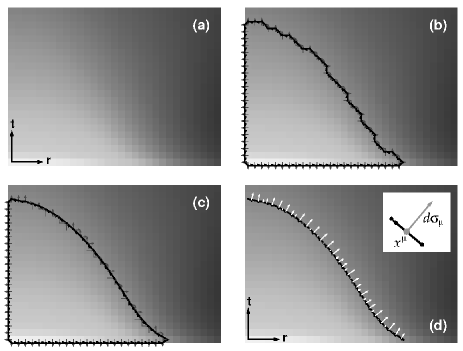
Figure 14: (a) A gray-level image representing the temporal temperature evolution of a 1D relativistic fluid (see text); (b) a dilated contour encloses pixels with temperatures $T\geq T_{f}$ and corresponding range vectors; (c) as in (b), but after contour displacement with respect to the fluid temperatures; (d) final FOHS with normal vectors $d\sigma_{\mu}(x^{\mu})$.

A FOHS is considered to be a lower-dimensional interface representing the union of all subatomic particle production events. In 3+1D (i.e., 3D space plus 1D time) hydrodynamic simulations, a FOHS is a 3D volume which is embedded in the 4D space-time. Events of subatomic particle production take place at a space-time $4$-vector, $x^{\mu}$ ($\mu=0,1,2,3$), on the FOHS. The index $\mu=0$ typically refers to the temporal dimension and the indices $\mu=1,2,3$ refer to the three spatial dimensions, respectively. If one intends to calculate probability distribution functions for the production of hadrons, one has to know further quantities REF44 ; REF45 . These are, e.g., the $4$-normal vector of the FOHS, $d\sigma_{\mu}(x^{\mu})$, the $4$-velocity vector of the fluid at freeze-out, $u_{\mu}(x^{\mu})$, the temperature at freeze-out, $T_{f}(x^{\mu})$, etc. Very often, the FOHS is assumed to be an hyper-isosurface with respect to the temperature field REF43 –REF45 of the relativistic fluid, i.e., $T_{f}(x^{\mu})=T_{f}=const$. The exploitation of spatial symmetries may allow the physicist to investigate certain aspects of relativistic fluid dynamics simulations in reduced dimensions, such as in a 1D radial space plus 1D time. Then the problem of FOHS extraction becomes identical to a 1D thermal isocontour extraction on a discretized 2D hydrodynamic simulation history. The 2D hydrodynamic simulation history is comprized of a discretized 1+1D space-time lattice (similar to 2D image data), on which field quantities such as temperature or fluid velocity components, etc., have been stored.
Fig. 14.a shows a 2D hydrodynamic simulation history of the discrete fluids temperature field, i.e., the temporal temperature evolution of a 1D relativistic fluid. In other words, Fig. 14.a is an image, $T=T(t,r)$, where $T$, $t$, and $r$ are the (continuous) fluid temperature, the (discretized) time and a (discretized) spatial dimension (e.g., radius, because a radial symmetry may apply), respectively. Darker pixels refer to lower fluid temperatures, whereas brighter ones refer to higher fluid temperatures. The origin of the space-time lattice (i.e., $r=t=0$) is located in the center of the lower left image pixel. The FOHS is defined here as a thermal isocontour of value $T_{f}$ and is constructed as follows. First, all lattice points (i.e., pixels) which have a temperature higher or equal to $T_{f}$ are enclosed with a left-turning (i.e., pixel disconnecting) DICONEX contour. This is depicted in Fig. 14.b, which also shows the range vectors neccessary for the following isocontour extraction. In the next step, the isocontour is constructed (cf., Fig. 14.c). When the contour support points are relocated through linear interpolation, the corresponding field quantities such as fluid velocity field components, etc., are evaluated for the isocontour supporting points as well. Note, that points which sit directly on the boundary of the image data are not moved. Contour edges which have both supporting points with coordinates $r\leq 0$ and/or $t\leq 0$, are physically irrelevant (for reasons, which are not explained here). They have been removed in the final result shown in Fig. 14.d. In Fig. 14.d, we also show the corresponding $4$-normal vectors of the FOHS at freeze-out, $d\sigma_{\mu}(x^{\mu})$. Note, that in 1+1D these $4$-vectors are just the normal vectors of the isocontour vectors REF46 . Furthermore, the 1+1D freeze-out events, $x^{\mu}=(t_{f},r_{f})$, are associated with the middle of each isocontour vector (cf., Fig. 14.d), and so are all corresponding field quantities (i.e., $d\sigma_{\mu}(x^{\mu})$, $u_{\mu}(x^{\mu})$, etc.). $t_{f}$ and $r_{f}$ denote the freeze-out times and freeze-out radii, respectively.

IV Summary

In summary, we have introduced a new framework for 1D contour extraction from discrete 2D data sets. Within this toolbox approach, we can generate up to five different types of contours. These are (i) the contours made up by the connected sets of contour vectors which initially separate pairs of pixels, (ii) DICONEX or dilated contours, (iii) boundary pixel tracing contours, (iv) isocontours, and (v) contours from shape skeletons, respectively. All of the contours can be computed rather fast and 100% robustly. In particular, the DICONEX contours resemble a class of perfect contours in the sense that they are always non-selfintersecting and non-degenerate, i.e., they always enclose an area larger than zero.
An important integral part of the contour extraction toolbox is a constrained Delaunay tessellation tool, which aids the gap closure and/or continuation of contour fragments such that closed contours may be obtained at all times. The Delaunay tessellations are also useful for contour simplification (cf., Ref. REF17 ), as well as extraction and potential pruning of shape skeletons. The introduction of high-level shape constituents (e.g., torsos) allow for contour refinement through 2D shape manipulations.
Finally, we have demonstrated that a wide range of rather diverse applications can be addressed with this novel contour extraction framework.

V Acknowledgements

This work has been supported by the Department of Energy under contract W-7405-ENG-36.

References

- (1) S. Di Zenzo, L. Cinque, and S. Levialdi, “Run-Based Algorithms for Binary Image Analysis and Processing,” IEEE Transactions on Pattern Analysis and Machine Intelligence, 18 (1996) 83 – 89.
- (2) E. Bribiesca, “A new chain code,” Pattern Recognition, 32 (1999) 235 – 251.
- (3) N. L. Jones, M. J. Kennard, A. K. Zundel, “Fast algorithm for generating sorted contour strings,” Computers and Geosciences, 26 (2000) 831 – 837.
- (4) S. Kaygin, M. M. Bulut, “A new one-pass algorithm to detect region boundaries,” Pattern Recognition Letters, 22 (2001) 1169 – 1178.
- (5) Y. B. Bai, X. W. Xu, “Object Boundary Encoding – a new vectorisation algorithm for engineering drawings,” Computers in Industry, 46 (2001) 65 – 74.
- (6) M. Ren, J. Yang, H. Sun, “Tracing boundary contours in a binary image,” Image and Vision Computing, 20 (2002) 125 – 131.
- (7) T. Pavlidis, Algorithms for Graphics and Image Processing, Computer Science Press, 1982, 142 – 148.
- (8) W. K. Pratt, Digital Image Processing, John Wiley & Sons, 2001.
- (9) J. R. Parker, Algorithms for Image Processing and Computer Vision, John Wiley & Sons, 1997.
- (10) B. Jähne, Digital Image Processing, Springer, 1997.
- (11) J. Canny, “A Computational Approach to Edge Detection,” IEEE Transactions on Pattern Analysis and Machine Intelligence, PAMI-8 (1986) 679 – 698.
- (12) B. R. Schlei, L. Prasad, “A Parallel Algorithm for Dilated Contour Extraction from Bilevel Images,” Los Alamos Preprint LA-UR-00-309, Los Alamos National Laboratory, cs.CV/0001024, 2000.
- (13) P. L. George and H. Borouchaki, Delaunay Triangulation and Meshing, Hermes, 1998.
- (14) B. R. Schlei, “DICONEX - Dilated Contour Extraction Code, Version 1.0,” Los Alamos Computer Code LA-CC-00-30, Los Alamos National Laboratory.
- (15) B. R. Schlei, L. Prasad and A. N. Skourikhine, “Geometric Morphology of Granular Materials,” Proceedings of SPIE 2000, 4117 (2000) 196 – 201.
- (16) B. R. Schlei, L. Prasad and A. N. Skourikhine, “Geometric morphology of cellular solids,” Proceedings of SPIE 2001, 4476 (2001) 73 – 79.
- (17) B. R. Schlei, “Region-Enclosing Contours from Edge Pixels,” Vision Geometry XI, Proceedings of SPIE’s Annual Meeting, Seattle, WA, 4794 (2002) 63 – 70.
- (18) L. Prasad, “Morphological Analysis of Shapes,” CNLS Newsletter, No. 139, July ‘97, LALP-97-010-139, Center for Nonlinear Studies, Los Alamos National Laboratory.
- (19) L. Prasad, R. Rao, “A Geometric Transform for Shape Feature Extraction,” Proceedings of SPIE 2000, 4117 (2000) 222 – 233.
- (20) J. J. Zou, H.-H. Chang, H. Yan, “Shape skeletonization by identifying discrete local symmetries,” Pattern Recognition, 34 (2001) 1895 – 1905.
- (21) B. R. Schlei, “Counting Bacterial Colonies,” Theoretical Division - Self Assessment, Special Feature, a portion of LA-UR-02-1409, Los Alamos (2002) 113 – 114.
- (22) L. Prasad, R. Rao, “Multi-scale Discretization of Shape Contours,” Proceedings of SPIE 2000, 4117 (2000) 202 – 209.
- (23) L. J. Latecki, R. Lakämper, “Convexity rule for shape decomposition based on discrete contour evolution,” Comput. Vision Image Understanding, 73 (1999) 441 – 454.
- (24) L. J. Latecki, R. Lakämper, “Application of planar shape comparison to object retrieval in image databases,” Pattern Recognition, 35 (2002) 15 – 29.
- (25) M. C. Demirel, B. S. El-Dasher, B. L. Adams, A. D. Rollet, “Studies on the Accuracy of Electron Backscatter Diffraction Measurements,” Electron Backscatter Diffraction in Materials Science, Kluwer Academic-Plenum Publishers, New York, 2000, 65 - 74.
- (26) A. Kuprat, D. George, G. Straub, M. C. Demirel, “Modeling microstructure in three dimensions with Grain3D and LaGrit,” Comp. Mat. Sci. 28 (2003) 199 – 208.
- (27) courtesy, M. C. Demirel, Department of Engineering Science and Mechanics, Pennsylvania State University, PA.
- (28) D. T. Carpenter, J. M. Rickman, and K. Barmak, “A methodology for automated quantitative microstructural analysis of transmission electron micrographs,” J. Appl. Phys., 84 (1998) 5843 – 5854.
- (29) J. Wilson, T. Hunt, Molecular Biology of the Cell: A Problems Approach, Garland Science, 2002.
- (30) courtesy, B. Kirkup, Osborne Memorial Laboratory, Yale University, New Haven, CT.
- (31) L. da F. Costa and R. M. Cesar Jr., Shape Analysis and Classification: Theory and Practice, CRC Press, 2000.
- (32) M. de Berg, M. van Kreveld, M. Overmars, O. Schwarzkopf, Computational Geometry: Algorithms and Applications, Springer, 1997.
- (33) R. Diestel, Graphentheorie, Springer, 2006.
- (34) L. Prasad, A. N. Skourikhine, and B. R. Schlei, “Feature-based Syntactic and Metric Shape Recognition,” Proceedings of SPIE 2000, 4117 (2000) 234 – 242.
- (35) B. R. Schlei, L. Prasad, and A. N. Skourikhine,“Syntactic Shape Description,” Theoretical Division - Self Assessment, Special Feature, a portion of LA-UR-01-1847, Los Alamos (2001) 58 – 59.
- (36) J. P. Marques de S\a’a, Pattern Recognition, Springer, 2001.
- (37) A. Weigert and H. J. Wendker, Astronomie und Astrophysik: ein Grundkurs, VCH, 1989.
- (38) M. Fineman, The Nature of Visual Illusion, Dover, 1996.
- (39) J. O’Rourke, Computational Geometry in C, Cambridge, 1993.
- (40) E. B. Goldstein, Wahrnehmungspsychologie, Spektrum, Akad. Ver., 2002.
- (41) R. B. Clare, D. Strottman, “Relativstic Hydrodynamics and Heavy Ion Collisions,” Phys. Rep. 141 (1986) 177 – 280.
- (42) L. P. Csernai, Introduction to Relativistic Heavy Ion Collisions, John Wiley & Sons, 1994.
- (43) F. Cooper, G. Frye, E. Schonberg, “Landau’s hydrodynamic model of particle production and electron-positron annihilation into hadrons,” Phys. Rev. D11 (1975) 192 – 213.
- (44) J. Bolz, U. Ornik, R. M. Weiner, “Relativistic hydrodynamics of partially stopped baryonic matter,” Phys. Rev. C46 (1992) 2047 – 2056.
- (45) J. Bolz, U. Ornik, M. Plümer, B. R. Schlei, R. M. Weiner, “Resonance decays and partial coherence in Bose-Einstein correlations,” Phys. Rev. D47 (1993) 3860 – 3870.
- (46) E. M. Lifschitz, L. D. Landau, The Classical Theory of Fields: Volume 2, Butterworth-Heinemann, 1980.