Computing Multi-Homogeneous Bézout Numbers is Hard

Gregorio Malajovich¹¹1 Postal address: Departamento de Matemática Aplicada, Universidade Federal do Rio de Janeiro. Caixa Postal 68530, CEP 21945-970, Rio de Janeiro, RJ, Brasil. email:gregorio@ufrj.br. url: www.labma.ufrj.br//~gregorio. Acknowledgements: G.M. is partially supported by CNPq (Brasil). This work was done while visiting Syddansk Universitet at Odense, thanks to the generous support of the Villum Kann Rasmussen Fond.
Klaus Meer ²²2Postal address: Department of Mathematics and Computer Science. University of Southern Denmark, Campusvej 55, DK-5230, Odense M. Denmark. email:meer@imada.sdu.dk. url: www.imada.sdu.dk//~meer. Acknowledgements: Partially supported by the EU Network of Excellence PASCAL Pattern Analysis, Statistical Modelling and Computational Learning and by the Danish Natural Science Research Council SNF.

(29 april 2004)

Abstract

The multi-homogeneous Bézout number is a bound for the number of solutions of a system of multi-homogeneous polynomial equations, in a suitable product of projective spaces.

Given an arbitrary, not necessarily multi-homogeneous system, one can ask for the optimal multi-homogenization that would minimize the Bézout number.

In this paper, it is proved that the problem of computing, or even estimating the optimal multi-homogeneous Bézout number is actually $\mathbf{NP}$ -hard.

In terms of approximation theory for combinatorial optimization, the problem of computing the best multi-homogeneous structure does not belong to $\mathbf{APX}$ , unless $\mathbf{P}=\mathbf{NP}$ .

Moreover, polynomial time algorithms for estimating the minimal multi-homogeneous Bézout number up to a fixed factor cannot exist even in a randomized setting, unless $\mathbf{BPP}\supseteq\mathbf{NP}$ .

1 Introduction

The multi-homogeneous Bézout number is a bound for the number of solutions of a system of multi-homogeneous polynomial equations.

Estimating the number of isolated solutions of a polynomial system is useful for the design and analysis of homotopy algorithms [LI]. Applications include problems in engineering like the design of certain mechanisms [MORGAN, WMS] or others, such as computational geometry.

An application of multi-homogeneous Bézout bounds outside the realm of algebraic equation solving is discussed in [DMS], where the number of roots is used to bound geometrical quantities such as volume and curvature.

There is an important connection between root-counting and $\mathbf{NP}$ -completeness theory. Indeed, it is easy to reduce an $\mathbf{NP}$ -complete or $\mathbf{NP}$ -hard problem such as SAT, the Traveling Salesman problem, Integer Programming (and thus all other $\mathbf{NP}$ problems as well) to the question whether certain polynomial systems have a common zero.

The best-known example giving an estimate for the number of roots of a polynomial equation is the Fundamental Theorem of Algebra. It was generalized to multivariate polynomial systems at the end of the 18th century by Etienne Bézout. The Bézout number bounds the number of (isolated) complex solutions of a polynomial $f:\mathbb{C}^{n}\mapsto\mathbb{C}^{n}$ from above by the product of the degrees of the involved polynomials. However, in many cases this estimate is far from optimal. A well known example is given by the eigenvalue problem: Given a $n\times n$ matrix $M$ , find the eigenpairs $(\lambda,u)\in\mathbb{C}\times\mathbb{C}^{n}$ such that $Mu-\lambda u=0$ . If we equate $u_{n}$ to $1$ , the classical Bézout number becomes $2^{n-1},$ though of course only $n$ solutions exist.

The multi-homogeneous Bézout number provides a sharper bound on the number of isolated solutions of a system of equations, in a suitable product of projective spaces. The multi-homogeneous Bézout bound depends on the choice of a multi-homogeneous structure, that is of a partition of the variables $(\lambda,u)$ into several groups.

In the eigenvalue example, the eigenvector $u$ is defined up to a multiplicative constant, so it makes sense to define it as an element of $\mathbb{P}^{n-1}$ . With respect to the eigenvector $\lambda$ , we need to introduce a homogenizing variable. We therefore rewrite the equation as: $\lambda_{0}Mu-\lambda_{1}u=0$ , and $\lambda=\lambda_{1}/\lambda_{0}$ . Now the pair $(\lambda_{0}:\lambda_{1})$ is an element of $\mathbb{P}^{1}$ . The multi-homogeneous Bézout number for this system is precisely $n$ .

Better bounds on the root number are known, such as Kushnirenko’s [KUSHNIRENKO] or Bernstein’s [BERNSTEIN]. However, interest in computing the multi-homogeneous Bézout number stems from the fact that hardness results are known for those sharper bounds (see section 2.2 for details).

Another reason of interest is that in many cases, a natural multi-homogeneous structure is known or may be found with some additional human work.

In this paper, we consider the following problem. Let $n\in\mathbb{N}$ and a finite $A\subset\mathbb{N}^{n}$ be given as input. Find the minimal multi-homogeneous Bézout number, among all choices of a multi-homogeneous structure for a polynomial system with support $A$ :

\left\{\begin{array}[]{lcl}f_{1}(z)&=&\sum_{\mathbf{\boldsymbol{\alpha}}\in A}f_{1\mathbf{\boldsymbol{\alpha}}}z_{1}^{\alpha_{1}}z_{2}^{\alpha_{2}}\cdots z_{n}^{\alpha_{n}}\\ &\vdots&\\ f_{n}(z)&=&\sum_{\mathbf{\boldsymbol{\alpha}}\in A}f_{n\mathbf{\boldsymbol{\alpha}}}z_{1}^{\alpha_{1}}z_{2}^{\alpha_{2}}\cdots z_{n}^{\alpha_{n}}\ .\\ \end{array}\right.

(1)

where the $f_{i\mathbf{\alpha}}$ are non-zero complex coefficients.

Geometrically, this minimal Bézout number is an upper bound for the number of isolated roots of the system (1) in $\mathbb{C}^{n}$ .

The main result in this paper (restated formally in section 2.1 below) is:

Theorem 1.

There cannot possibly exist a polynomial time algorithm to approximate the minimal multi-homogeneous Bézout number for (1) up to any fixed factor, unless $\mathbf{P}=\mathbf{NP}$ .

This means that computing or even approximating the minimal Bézout number up to a fixed factor is $\mathbf{NP}$ -hard. In terms of the hierarchy of approximation classes (see [AUSIELLO] and section 2.4), the minimal multi-homogeneous Bézout number does not belong to the class $\mathbf{APX}$ unless $\mathbf{P}=\mathbf{NP}$ .

Motivated by what is known on volume approximation (see section 2.2), one could ask whether allowing for randomized algorithms would be of any improvement.

Theorem 2.

There cannot possibly exist a randomized polynomial time algorithm to approximate the minimal multi-homogeneous Bézout number for (1) up to any fixed factor, with probability of failure $\epsilon<1/4$ , unless $\mathbf{BPP}\supseteq\mathbf{NP}$ .

While the conjecture $\mathbf{BPP}\not\supseteq\mathbf{NP}$ is less widely known outside the computer science community than the conjecture $\mathbf{P}\neq\mathbf{NP}$ , its failure would imply the existence of probabilistic polynomial time algorithms for solving problems such as the factorization of large integers or the discrete logarithm. Most widespread cryptographic schemes are based on the assumption that those two problems are hard.

2 Background and Statement of Main Results

2.1 Bézout numbers

In the definition of (1), we assumed for simplicity that each equation had the same support $A$ . In general, a system $f(z)$ of $n$ polynomial equations with support $(A_{1},\dots,A_{n})$ is a system of the form:

\left\{\begin{array}[]{lcl}f_{1}(z)&=&\sum_{\boldsymbol{\alpha}\in A_{1}}f_{1\mathbf{\boldsymbol{\alpha}}}z_{1}^{\alpha_{1}}z_{2}^{\alpha_{2}}\cdots z_{n}^{\alpha_{n}}\\ &\vdots&\\ f_{n}(z)&=&\sum_{\boldsymbol{\alpha}\in A_{n}}f_{n\mathbf{\boldsymbol{\alpha}}}z_{1}^{\alpha_{1}}z_{2}^{\alpha_{2}}\cdots z_{n}^{\alpha_{n}}\ ,\\ \end{array}\right.

(2)

where the coefficients $f_{i\mathbf{\boldsymbol{\alpha}}}$ are non-zero complex numbers.

A multi-homogeneous structure is given by a partition of $\{1,\dots,n\}$ into (say) $k$ sets $I_{1},\dots,I_{k}$ . Then for each set $I_{j}$ , we consider the group of variables $Z_{j}=\{z_{i}:i\in I_{j}\}$ .

The degree of $f_{i}$ in the group of variables $Z_{j}$ is

d_{ij}\stackrel{{\scriptstyle\mbox{\scriptsize def}}}{{=}}\max_{\boldsymbol{\alpha}\in A_{i}}\ \sum_{l\in I_{j}}\ \alpha_{l}

When for some $j$ , for all $i$ , the maximum $d_{ij}$ is attained for all $\boldsymbol{\alpha}\in A_{i}$ , we say that (2) is homogeneous in the variables $Z_{j}$ . The dimension of the projective space associated to $Z_{j}$ is:

a_{j}\stackrel{{\scriptstyle\mbox{\scriptsize def}}}{{=}}\left\{\begin{array}[]{ll}\#I_{j}-1&\text{if (\ref{eq:**}) is homogeneous in $Z_{j}$, and}\\ \#I_{j}&\text{otherwise.}\end{array}\right.

We assume that $n=\sum_{j=1}^{k}a_{j}$ . Otherwise, we would have an undetermined ( $n<\sum_{j=1}^{k}a_{j}$ ) or overdetermined ( $n>\sum_{j=1}^{k}a_{j}$ ) polynomial system, and multi-homogeneous Bézout numbers would have no meaning.

The multi-homogeneous Bézout number $\mathrm{B\acute{e}z}(A_{1},\dots,A_{n};I_{1},\dots,I_{k})$ is the coefficient of $\prod_{j=1}^{k}\zeta_{j}^{a_{j}}$ in the formal expression $\prod_{i=1}^{n}\sum_{j=1}^{k}d_{ij}\zeta_{j}$ (see [MORGAN-SOMMESE, LI, SHAFAREVICH]). It bounds the maximal number of isolated roots of (2) in $\mathbb{P}^{a_{1}}\times\cdots\times\mathbb{P}^{a_{k}}$ . Therefore it also bounds the number of finite roots of (2), i.e. the roots in $\mathbb{C}^{n}$ .

In the particular case where $A=A_{1}=\cdots=A_{n}$ there is a simpler expression for the multi-homogeneous Bézout number $\mathrm{B\acute{e}z}(A;I_{1},\dots,I_{k})\stackrel{{\scriptstyle\mbox{\scriptsize def}}}{{=}}\mathrm{B\acute{e}z}(A_{1},\dots,A_{n};$ $I_{1},\dots,I_{k})$ , namely:

\mathrm{B\acute{e}z}(A;I_{1},\dots,I_{k})={\left(\begin{array}[]{c}n\\ a_{1}\ a_{2}\ \cdots\ a_{k}\end{array}\right)}\ \prod_{j=1}^{k}d_{j}^{a_{j}}\ ,

(3)

where $d_{j}=d_{ij}$ (equal for each $i$ ) and the multinomial coefficient

{\left(\begin{array}[]{c}n\\ a_{1}\ a_{2}\ \cdots\ a_{k}\end{array}\right)}\stackrel{{\scriptstyle\mbox{\scriptsize def}}}{{=}}\frac{n!}{a_{1}!\ a_{2}!\ \cdots\ a_{k}!}

is the coefficient of $\prod_{j=1}^{k}\zeta_{j}^{a_{k}}$ in $(\zeta_{1}+\cdots+\zeta_{k})^{n}$ (recall that $n=\sum_{j=1}^{k}a_{j}$ ).

Heuristics for computing a suitable multi-homogeneous structure $(I_{1},\dots,I_{k})$ given $A_{1},\dots,A_{n}$ are discussed in [LI-BAI, LI-LIN-BAI]. Surprisingly enough, there seems to be no theoretical results available on the complexity of computing the minimal Bézout number. It was conjectured in [LI-BAI, p.78] that computing the minimal multi-homogeneous Bézout number is $\mathbf{NP}$ -hard.

Even, no polynomial time algorithm for computing the multi- homogeneous Bézout number given a multi-homogeneous structure seems to be known (see [LI-LIN-BAI, p.240]).

This is why in this paper, we restrict ourselves to the case $A=A_{1}=\cdots=A_{n}$ . This is a particular subset of the general case, and any hardness result for this particular subset implies the same hardness result in the general case.

More formally, we adopt the Turing model of computation and we consider the function:

\mathrm{B\acute{e}z}:n,k,A,I_{1},\dots,I_{k}\mapsto\mathrm{B\acute{e}z}(A;I_{1},\dots,I_{k})

where all integer numbers are in binary representation, and $A$ is a list of $n$ -tuples $(\alpha_{1},\dots,\alpha_{n})$ , and each $I_{j}$ is a list of its elements. In particular, the input size is bounded below by $n\#A_{i}$ and by $\max_{\boldsymbol{\alpha},i}\lceil\log_{2}\alpha_{i}\rceil$ . Therefore, $\mathrm{B\acute{e}z}(A;I_{1},\cdots,I_{k})$ can be computed in polynomial time by a straight-forward application of formula (3). As a matter of fact, it can be computed in time polynomial in the size of $A$ .

Problem 1 (Discrete optimization problem).

Given $n$ and $A$ , compute

\min_{\boldsymbol{I}}\mathrm{B\acute{e}z}(A;{\boldsymbol{I}})\ ,

where $\boldsymbol{I}=(I_{1},\dots,I_{k})$ ranges over all the partitions of $\{1,\dots,n\}$ .

Problem 2 (Approximation problem).

Let $C>1$ be fixed. Given $n$ and $A$ , compute some $B$ such that

BC^{-1}<\min\mathrm{B\acute{e}z}(A;\boldsymbol{I})<BC

Again, $\boldsymbol{I}=(I_{1},\dots,I_{k})$ ranges over all the partitions of $\{1,\dots,n\}$ .

In the problems above, we are not asking for the actual partition.

Theorem 1 (restated).

Problem 2 is $\mathbf{NP}$ -hard.

This is actually stronger than the conjecture by Li and Bai [LI-BAI], that corresponds to the following immediate corollary:

Corollary 1.

Problem 1 is $\mathbf{NP}$ -hard.

2.2 Other bounds for the number of roots

Kushnirenko’s Theorem [KUSHNIRENKO] bounds the number of isolated solutions of (1) in $(\mathbb{C}^{*})^{n}$ by $n!\ \mathrm{Vol}\ \mathrm{Conv}A$ , where $\mathrm{Conv}A$ is the smallest convex polytope containing all the points of $A$ .

This bound is sharper than the Bézout bound, but the known hardness results are far more dramatic: In [KHACHIYAN], Khachiyan proved that computing the volume of a polytope given by a set of vertices is $\mathbf{\#P}$ -hard.

There is a large literature on algorithms for approximating the volume of a convex body given by a separation oracle. The problem of approximating the volume of a polytope in vertex representation can be reduced to the latter by standard linear programming techniques.

It is known that no deterministic algorithm can approximate the volume in polynomial time ([LOVASZ]). However, randomized polynomial time algorithms are known for the same problem [KLS, WW].

The same situation seems to be the case regarding the estimation of the mixed volume [DGH], which gives the actual number of solutions in $(\mathbb{C}^{*})^{n}$ for generic polynomials of the form (2) [BERNSTEIN].

2.3 Probabilistic algorithms

A probabilistic machine is a machine that has access to random bits of information, each random bit costing one unit of time. Each random bit is an independent, uniformly distributed random variable in $\{0,1\}$ . In that sense, a probabilistic machine is a machine that flips a fair coin, as many times as necessary, spending one unit of time at each flip.

We can therefore speak of the probability that the machine returns a correct result.

The class $\mathbf{BPP}$ is the class of decision problems $(X,X_{\mathrm{yes}})$ such that there is a probabilistic machine and a constant $\epsilon<1/2$ that will:

(i)

Decide in polynomial time if $x\in X$ .
(ii)

Output YES or NO, in polynomial time.
(iii)

For every $x$ , the output is the correct answer to the question: does $x\in X_{\mathrm{yes}}$ ? with probability $\geq 1-\epsilon$ .

Notice that we can improve the probability that the result is correct by running the same machine several times. Therefore, in the definition above, we may as well take $\epsilon=1/4$ .

More generally, a probabilistic machine solves a certain problem (e.g. Problem 2) in polynomial time with probability $\geq 1-\epsilon$ if and only if it always terminates in polynomial time, and the answer is correct with probability $1-\epsilon$ .

Theorem 2 (restated).

There is no $\epsilon<1/2$ and no probabilistic machine solving Problem 2 with probability $1-\epsilon$ , unless $\mathbf{BPP}\supseteq\mathbf{NP}$ .

2.4 Approximation classes

A theory of complexity classes appropriate for the study of combinatorial optimization problems is described in [AUSIELLO]. Problem 1 fits naturally in the class of combinatorial optimization problems. In this context, Problem 1 is characterized by:

(i)

A set of instances, given by the set of pairs $(n,A)$ , $n\in\mathbb{N},\ A\subset\mathbb{N}^{n}$ finite and non-empty.
(ii)

For every instance $(n,A)$ , a set of feasible solutions, namely the set of partitions ${\boldsymbol{I}}=(I_{1},\dots,I_{k})$ of $\{1,\dots,n\}$ .
(iii)

An objective function (to minimize), $\mathrm{B\acute{e}z}(A;{\boldsymbol{I}})$ .

The class $\mathbf{NPO}$ of combinatorial optimization problems is analogous to the class $\mathbf{NP}$ of decision problems. Problem 1 belongs to that class:

(1)

The size of each feasible solution is polynomially bounded on the size of each instance.
(2)

Given an instance $(n,A)$ and a string $w$ , it can be decided in time polynomial in $(n,A)$ whether $w$ encodes a feasible solution $\boldsymbol{I}=(I_{1},\dots,I_{k})$ .
(3)

The objective function can be computed in polynomial time.

The class $\mathbf{APX}$ of approximable problems in $\mathbf{NPO}$ is defined as the subset of $\mathbf{NPO}$ for which there is some $C>1$ and a polynomial time algorithm such that, given an instance of the problem (say $n,A$ )) produces a feasible solution $\boldsymbol{I}$ such that the objective function applied to that solution approximates the minimum up to a factor of $C$ .

Theorem 2 admits as a corollary:

Corollary 2.

Problem 1 does not belong to $\mathbf{APX}$ , unless $\mathbf{P}=\mathbf{NP}$ .

Our result actually holds even if we do not require the algorithms to compute a feasible solution.

3 Proof of the Main Theorems

3.1 From graph theory to systems of equations.

Definition 1.

A $k$ -coloring of a graph $G=(V,E)$ is a partition of the set of vertices $V$ into $k$ disjoint subsets (“colors”) $I_{j}$ , so that adjacent vertices do not belong to the same “color” $I_{j}$ .

Problem 3 (Graph 3-Coloring).

Given a graph $G=(V,E)$ , decide if there exists a $3$ -coloring of $G$ .

It is known since [KARP] that the Graph 3-Coloring Problem is $\mathbf{NP}$ -hard (see also [GAREY-JOHNSON]). We will actually need to consider an equivalent formulation of the Graph 3-coloring problem.

Recall that the cartesian product of two graphs $G_{1}=(V_{1},E_{1})$ and $G_{2}=(V_{2},E_{2})$ is the graph $G_{1}\times G_{2}=(V_{1}\times V_{2},E)$ with $((v_{1},v_{2}),(v_{1}^{\prime},v_{2}^{\prime}))\in E$ if and only if $v_{1}=v_{1}^{\prime}$ and $(v_{2},v_{2}^{\prime})\in E_{2}$ or $v_{2}=v_{2}^{\prime}$ and $(v_{1},v_{1}^{\prime})\in E_{1}$ .

Also, let $K_{3}$ denote the complete graph with 3 vertices.

Lemma 1.

The graph $G$ admits a 3-coloring if and only if the graph $G\times K_{3}$ admits a 3-coloring $\boldsymbol{I}=(I_{1},I_{2},I_{3})$ with $\#I_{1}=\#I_{2}=\#I_{3}=|G|$ .

Proof.

$G$ admits a 3-coloring if and only if $G\times K_{3}$ admits a 3-coloring. Moreover, any coloring $\boldsymbol{I}$ of $G\times K_{3}$ satisfies $\#I_{1}=\#I_{2}=\#I_{3}$ . ∎

To each graph $H=(V,E)$ we will associate two spaces of polynomial systems. Each of those spaces is characterized by a support set $A=A(H)$ (resp. $A(H)^{l}$ ) to be constructed and corresponds to the space of polynomials of the form (1) with complex coefficients. Of particular interest will be graphs of the form $H=G\times K_{3}$ .

We start by identifying the set $V$ of vertices of $H$ to the set $\{1,\dots,m\}$ . Let $K_{s}$ denote the complete graph of size $s$ , i.e. the graph with $s$ vertices all of them pairwise connected by edges.

To each copy of $K_{s}$ , $s=0,\dots,3$ that can be embedded as a subgraph of $H$ (say the subgraph generated by $\{v_{1},\cdots,v_{s}\}$ ) we associate the monomial

z_{v_{1}}z_{v_{2}}\cdots z_{v_{s}}

Refer to caption — Figure 1: In this example, $A(H)=\{(0,0,0,0),(1,0,0,0),(0,1,0,0),$ $(0,0,1,0),$ $(0,0,0,1),$ $(1,1,0,0),$ $(1,0,1,0),$ $(0,1,1,0),$ $(0,0,1,1),$ $(1,1,1,0)\}$ . A possible polynomial with that support would be $1+v_{1}+v_{2}+v_{3}+v_{4}+v_{1}v_{2}+v_{1}v_{3}+v_{2}v_{3}+v_{3}v_{4}+v_{1}v_{2}v_{3}$ .

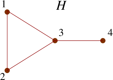
(the empty graph $K_{0}$ corresponds to the constant monomial). Then we consider the linear space generated by all those monomials (Figure 1). Therefore, the support $A(H)$ is the set of all $e_{v_{1}}+\cdots+e_{v_{s}}\subset\mathbb{N}^{m}$ such that $0\leq s\leq 3$ and $\{v_{1},\dots,v_{s}\}$ induces a copy of $K_{s}$ as a subgraph of $H$ . Here, $e_{i}$ denotes the $i$ -th vector of the canonical basis of $\mathbb{R}^{n}$ .

Given a set $A$ , we denote by $A^{l}$ the $l$ -fold i cartesian product of $A$ .

The two spaces of polynomial systems associated to a graph $H$ will be the polynomial systems with support $A(H)$ and $A(H)^{l}$ .

Remark that none of the two classes of systems above is homogeneous in any possible group of variables (because we introduced a constant monomial). Therefore, in the calculation of the Bézout number for a partition $\boldsymbol{I}$ , we can set $a_{j}=\#I_{j}$ .

Lemma 2.

Let $l$ be fixed. Then, there is a polynomial time algorithm to compute $A(H)$ and $A(H)^{l}$ , given $H$ .

3.2 A gap between Bézout numbers

In case the graph $H$ admits a $3$ -coloring $\boldsymbol{I}=(I_{1},I_{2},I_{3})$ , any corresponding polynomial system is always trilinear (linear in each set of variables). If moreover $H$ is of the form $H=G\times K_{3}$ with $|G|=n$ , the cardinality of the $I_{j}$ is always $n$ , and formula (3) becomes:

\mathrm{B\acute{e}z}(A(G\times K_{3});{\boldsymbol{I}})={\left(\begin{array}[]{c}3n\\ n\ n\ n\end{array}\right)}

The crucial step in the proof of Theorem 1 is to show that

\mathrm{B\acute{e}z}(A(G\times K_{3});{\boldsymbol{I}})\geq\frac{4}{3}{\left(\begin{array}[]{c}3n\\ n\ n\ n\end{array}\right)}

unless $k=3$ and ${\boldsymbol{I}}$ is a 3-coloring of $G\times K_{3}$ .

In order to do that, we introduce the following cleaner abstraction for the Bézout number: if $k\in\mathbb{N}$ and ${\mathbf{a}}=(a_{1},\dots,a_{k})\in\mathbb{N}^{k}$ are such that $\sum_{j=1}^{k}a_{j}=3n$ , we set

B(\mathbf{a})\stackrel{{\scriptstyle\mbox{\scriptsize def}}}{{=}}{\left(\begin{array}[]{c}3n\\ a_{1}\ a_{2}\ \cdots\ a_{k}\end{array}\right)}\ \prod_{j=1}^{k}\left\lceil\frac{a_{j}}{n}\right\rceil^{a_{j}}

Lemma 3.

If $H=G\times K_{3}$ and ${\boldsymbol{I}}=(I_{1},\dots,I_{k})$ is a partition of the set $\{1,\dots,3n\}$ of vertices of $H$ , then

\mathrm{B\acute{e}z}(A(H);{\boldsymbol{I}})\geq B(\mathbf{a})

with $a_{j}=\#I_{j}$ .

Proof.

Consider the $n$ disjoint copies of $K_{3}$ in $H=G\times K_{3}$ induced by the nodes of $G$ . By the pigeonhole principle, there is at least one of those copies with at least $\lceil a_{j}/n\rceil$ elements of $I_{j}$ . Hence, the degree $d_{j}$ in the $j$ -th group of variables is at least $\lceil a_{j}/n\rceil$ . ∎

The main step towards establishing the “gap” is the following Proposition:

Proposition 1.

Let $n,k\in\mathbb{N}^{n}$ and let $a_{1}\geq a_{2}\geq\cdots\geq a_{k}\geq 1$ be such that $\sum_{j=1}^{k}a_{j}=3n$ . Then, either $k=3$ and $a_{1}=a_{2}=a_{3}=n$ , or:

B(\mathbf{a})\geq\frac{4}{3}B(n,n,n)\ .

Moreover, this bound is sharp.

The proof of Proposition 1 is postponed to section 4.

Putting it all together,

Lemma 4.

Let $G$ be a graph and $n=|G|$ . If $G$ admits a 3-coloring, then

\min_{\boldsymbol{I}}\mathrm{B\acute{e}z}(A(G\times K_{3});\boldsymbol{I})={\left(\begin{array}[]{c}3n\\ n\ n\ n\end{array}\right)}

Otherwise,

\min_{\boldsymbol{I}}\mathrm{B\acute{e}z}(A(G\times K_{3});\boldsymbol{I})\geq\frac{4}{3}{\left(\begin{array}[]{c}3n\\ n\ n\ n\end{array}\right)}

Proof.

According to Lemma 1, $G$ admits a 3-coloring if and only if $G\times K_{3}$ admits a 3-coloring.

If ${\boldsymbol{I}}=(I_{1},I_{2},I_{3})$ is a 3-coloring of $G\times K_{3}$ , then

\mathrm{B\acute{e}z}(A(G\times K_{3});\boldsymbol{I})={\left(\begin{array}[]{c}3n\\ n\ n\ n\end{array}\right)}

If $\boldsymbol{I}=(I_{1},\dots,I_{k})$ is not a 3-coloring of $G\times K_{3}$ , then we distinguish two cases.

We set $a_{j}=\#I_{j}$ .

Case 1: ${\mathbf{a}}=(n,n,n)$ and hence $k=3$ . Then the degree in at least one group of variables is $\geq 2$ , and

\mathrm{B\acute{e}z}(A(G\times K_{3});\boldsymbol{I})\geq 2^{n}{\left(\begin{array}[]{c}3n\\ n\ n\ n\end{array}\right)}

Case 2: ${\mathbf{a}}\neq(n,n,n)$ . Then

\mathrm{B\acute{e}z}(A(G\times K_{3});\boldsymbol{I})\geq B(a_{1},\dots,a_{k})\geq\frac{4}{3}{\left(\begin{array}[]{c}3n\\ n\ n\ n\end{array}\right)}\ ,

where the first inequality follows from Lemma 3 and the second from Proposition 1.

In both cases,

\min_{\boldsymbol{I}}\mathrm{B\acute{e}z}(A(G\times K_{3}),\boldsymbol{I})\geq\frac{4}{3}{\left(\begin{array}[]{c}3n\\ n\ n\ n\end{array}\right)}.

∎

Lemma 4 would be sufficient to prove a weaker version of Theorem 1, where the factor $C$ in problem 2 is less than $4/3$ .

3.3 Improving the gap

In order to obtain a proof valid for any $C$ the idea is to increase the gap by considering several copies of a polynomial system, but each copy in a new set of variables. This idea works out because of the special multiplicative structure of the multi-homogeneous Bézout number. We will need:

Proposition 2.

Let $m,l\in\mathbb{N}$ . Let $A\subset\mathbb{N}^{m}$ be finite and assume that $0\in A$ . Then,

\min_{\boldsymbol{J}}\mathrm{B\acute{e}z}(A^{l};\boldsymbol{J})={\left(\begin{array}[]{c}lm\\ m\ m\ \cdots\ m\end{array}\right)}\ \left(\min_{\boldsymbol{I}}\mathrm{B\acute{e}z}(A;\boldsymbol{I})\right)^{l}

Proof.

1. Let $\boldsymbol{I}=(I_{1},\cdots,I_{k})$ be the partition of $\{1,\dots,m\}$ where the minimal Bézout number for $A$ is attained.

This induces a partition $\boldsymbol{J}=(J_{js})_{1\leq j\leq k,1\leq s\leq l}$ of $\{1,\dots,m\}\times\{1,\dots,l\}$ , given by $J_{js}=I_{j}\times\{s\}$ . Identifying each pair $(i,s)$ with $i+ms$ , the $J_{js}$ are also a partition of $\{1,\dots,lm\}$ .

By construction of $A^{l}$ , the degree $d_{js}$ in the variables corresponding to $J_{js}$ is equal to the degree $d_{j}$ of the variables $I_{j}$ in $A$ .

The systems corresponding to $A$ and $A^{l}$ cannot be homogeneous for any partition, since $0\in A$ and $0\in A^{l}$ . Then we have $a_{j}=\#I_{j}=a_{js}$ for any $s$ . Therefore,

$\displaystyle\min_{\boldsymbol{K}}\mathrm{B\acute{e}z}(A^{l},\boldsymbol{K})$	$\displaystyle\leq$	$\displaystyle\mathrm{B\acute{e}z}(A^{l},\boldsymbol{J})$
	$\displaystyle=$	$\displaystyle{\left(\begin{array}[]{c}lm\\ \underbrace{a_{1}\ \cdots\ a_{1}}_{l\text{\ times}}\ \cdots\ \underbrace{a_{k}\ \cdots\ a_{k}}_{l\text{\ times}}\end{array}\right)}\prod_{s=1}^{l}\prod_{j=1}^{k}d_{j}^{a_{j}}$
	$\displaystyle=$	$\displaystyle{\left(\begin{array}[]{c}lm\\ m\ m\ \cdots\ m\end{array}\right)}\ \left({\left(\begin{array}[]{c}m\\ a_{1}\ a_{2}\ \cdots\ a_{k}\end{array}\right)}\prod_{j=1}^{k}d_{j}^{a_{j}}\right)^{l}$
	$\displaystyle=$	$\displaystyle{\left(\begin{array}[]{c}lm\\ m\ m\ \cdots\ m\end{array}\right)}\ \left(\min_{\boldsymbol{I}}\mathrm{B\acute{e}z}(A;\boldsymbol{I})\right)^{l}$

2. Now, suppose that the minimal Bézout number for $A^{l}$ is attained for a partition $\boldsymbol{J}=(J_{1},\cdots,J_{r})$ . We claim that each $J_{t}$ fits into exactly one of the $l$ sets $\{1,\dots,m\}\times\{s\}$ .

Suppose this is not the case. Assume without loss of generality that $J_{1}$ splits into $K\subset\{1,\dots,m\}\times\{1\}$ and $L\subset\{1,\dots,m\}\times\{2,\dots,l\}$ , both $K$ and $L$ non-empty.

If $d_{K}$ denotes the degree in the $K$ -variables and $d_{L}$ the degree in the $L$ variables, then $d_{1}=d_{K}+d_{L}$ . Also, $a_{1}=a_{K}+a_{L}$ where $a_{K}$ is the size of $K$ and $a_{L}$ is the size of $L$ . The multi-homogeneous Bézout number corresponding to the partition ${\boldsymbol{J}^{\prime}}=(K,L,J_{2},\cdots,J_{r})$ is:

\mathrm{B\acute{e}z}(A^{l};\boldsymbol{J}^{\prime})={\left(\begin{array}[]{c}3lm\\ a_{K}\ a_{L}\ a_{2}\ \cdots\ a_{r}\end{array}\right)}d_{K}^{a_{K}}d_{L}^{a_{L}}\prod_{j=2}^{r}d_{j}^{a_{j}}

Therefore,

\frac{\mathrm{B\acute{e}z}(A^{l};\boldsymbol{J}^{\prime})}{\mathrm{B\acute{e}z}(A^{l},\boldsymbol{J})}=\frac{{\left(\begin{array}[]{c}a_{1}\\ a_{K}\end{array}\right)}d_{K}^{a_{K}}d_{L}^{a_{L}}}{(d_{K}+d_{L})^{a_{1}}}<1

and the Bézout number was not minimal, thus establishing the claim.

3. Denote by $\boldsymbol{J}=\cup_{s=1}^{l}\boldsymbol{J}^{(s)}$ the partition minimizing the Bézout number corresponding to $A^{l}$ . In the notation above, we assume that ${\boldsymbol{J}^{(s)}}$ is a partition of $\{1,\dots,m\}\times\{s\}$ .

In that case,

$\displaystyle\mathrm{B\acute{e}z}(A^{l};\boldsymbol{J})$	$\displaystyle=$	$\displaystyle{\left(\begin{array}[]{c}lm\\ m\ m\ \cdots\ m\end{array}\right)}\prod_{s=1}^{l}\left({\left(\begin{array}[]{c}m\\ a_{1}^{(s)}\ \cdots\ a_{k}^{(s)}\end{array}\right)}\prod_{j=1}^{k}(d_{j}^{(s)})^{a_{j}^{(s)}}\right)$
	$\displaystyle=$	$\displaystyle{\left(\begin{array}[]{c}lm\\ m\ m\ \cdots\ m\end{array}\right)}\prod_{s=1}^{l}\mathrm{B\acute{e}z}(A,\boldsymbol{J}^{(s)})$
	$\displaystyle\geq$	$\displaystyle{\left(\begin{array}[]{c}lm\\ m\ m\ \cdots\ m\end{array}\right)}\left(\min_{\boldsymbol{I}}\mathrm{B\acute{e}z}(A;\boldsymbol{I})\right)^{l}$

∎

Combining Lemma 4 and Proposition 2, we established that:

Lemma 5.

Let $G$ be a graph and $n=|G|$ . Let $l\in\mathbb{N}$ . If $G$ admits a 3-coloring, then

\min_{\boldsymbol{J}}\mathrm{B\acute{e}z}(A(G\times K_{3})^{l},\boldsymbol{J})={\left(\begin{array}[]{c}3nl\\ 3n\ 3n\ \cdots\ 3n\end{array}\right)}{\left(\begin{array}[]{c}3n\\ n\ n\ n\end{array}\right)}^{l}

Otherwise,

\min_{\boldsymbol{J}}\mathrm{B\acute{e}z}(A(G\times K_{3})^{l},\boldsymbol{J})\geq\left(\frac{4}{3}\right)^{l}{\left(\begin{array}[]{c}3nl\\ 3n\ 3n\ \cdots\ 3n\end{array}\right)}{\left(\begin{array}[]{c}3n\\ n\ n\ n\end{array}\right)}^{l}

Proof of Theorem 1.

Assume that ApproxBéz is a deterministic, polynomial time algorithm for solving problem 2, i.e., for estimating the Bézout number up to a factor of $C$ .

Then the following algorithm decides Graph 3-coloring (Problem 3) in polynomial time:

Algorithm 1 (Decides Graph 3-coloring problem).

Input: a graph $G$ of size $n$ .
Output: YES if $G$ admits a 3-coloring, NO otherwise.
Constants: $l=\left\lceil\frac{\log C}{2\log 4/3}\right\rceil$ .

Compute

\rho\leftarrow\frac{{\text{\sc ApproxB\'{e}z}}\left(A(G\times K_{3})^{l}\right)}{{\left(\begin{array}[]{c}3nl\\ 3n\ 3n\ \cdots\ 3n\end{array}\right)}{\left(\begin{array}[]{c}3n\\ n\ n\ n\end{array}\right)}^{l}}

2.

If $\rho^{2}<C$ then Output YES, else Output NO.

By our choice of the constant $l$ , $\sqrt{C}\leq(4/3)^{l}$ . Therefore, Lemma 5 asserts that the output of algorithm 1 is correct.

The bit-size of the numbers that occur when computing the denominator of line 2 are bounded above by $O(3nl\log(3nl))$ . The size of the graph $G\times K_{3}$ is $O(n)$ , and Lemma 2 says that $A^{l}$ can be computed in polynomial time.

It follows that Algorithm 1 runs in polynomial time. Since Graph 3-coloring is $\mathbf{NP}$ -complete, we deduce that $\mathbf{P}=\mathbf{NP}$ . ∎

Proof of Theorem 2.

Assume now that ApproxBéz is a probabilistic polynomial time algorithm for solving problem 2, which returns a correct result with probability $1-\epsilon$ , $\epsilon<1/4$ .

Then Algorithm 1 will return the correct answer for the Graph 3-coloring Problem, with probability at least $1-\epsilon$ . This implies that Problem 3 is actually in $\mathbf{BPP}$ . ∎

4 Proof of Proposition 1

We will need the following trivial Lemma in the proof of Proposition 1:

Lemma 6.

Let $x,n\in\mathbb{N}$ . Then,

\left(\left\lceil\frac{x}{n}\right\rceil\frac{n}{x}\right)^{x}\geq 1+\left(\rule{0.0pt}{8.61108pt}(n-x)\mod n\right)\ .

In particular, the left-hand side is $\geq 2$ whenever $n\not\>\mid x$ , and is always $\geq 1$ .

Proof.

Since $n\left\lceil\frac{x}{n}\right\rceil=x+(n-x)\mod n$ , we have:

\left(\left\lceil\frac{x}{n}\right\rceil\frac{n}{x}\right)^{x}=\left(1+\frac{(n-x)\mod n}{x}\right)^{x}\geq 1+\left(\rule{0.0pt}{8.61108pt}(n-x)\mod n\right)

∎

Also, we will make use of the Stirling Formula [HANDBOOK, (6.1.38)]:

x!=\sqrt{2\pi}\ x^{x+\frac{1}{2}}\ e^{-x+\frac{\theta(x)}{12x}}\ ,

(10)

where $0<\theta(x)<1$ .

Proof of Proposition 1.

The ratio between $B(\mathbf{a})$ and $B(n,n,n)$ is:

\frac{B(\mathbf{a})}{B(n,n,n)}=\prod_{j=1}^{k}\left\lceil\frac{a_{j}}{n}\right\rceil^{a_{j}}\ \frac{n!\ n!\ n!}{a_{1}!\ a_{2}!\ \cdots\ a_{k}!}

From Stirling formula (10) it follows immediately that:

\frac{B(\mathbf{a})}{B(n,n,n)}=\sqrt{2\pi}^{3-k}\ \prod_{j=1}^{k}\left\lceil\frac{a_{j}}{n}\right\rceil^{a_{j}}\ \frac{n^{3n+\frac{3}{2}}}{\prod_{j=1}^{k}a_{j}^{a_{j}+\frac{1}{2}}}\ e^{\frac{\theta(n)}{4n}-\sum\frac{\theta(a_{j})}{12a_{j}}}

(11)

Now we distinguish the cases $k=1$ , $k=2$ , and $k\geq 3$ . The first two cases are easy:

Case 1: If $k=1$ , then $a_{1}=3n$ and (11) becomes:

\frac{B(\mathbf{a})}{B(n,n,n)}=2\pi\ \frac{n}{\sqrt{3}}\ e^{\frac{\theta(n)}{4n}-\frac{\theta(3n)}{36n}}

which is bounded below by $\frac{2\pi}{\sqrt{3}}e^{-1/36}\simeq 3.528218766$ .

Case 2: If $k=2$ , Lemma 6 implies that

\frac{B(\mathbf{a})}{B(n,n,n)}\geq\sqrt{2\pi}\ \frac{n^{\frac{3}{2}}}{\sqrt{a_{1}\ a_{2}}}\ e^{-1/6}

Since $\sqrt{a_{1}\ a_{2}}\leq\frac{a_{1}+a_{2}}{2}=\frac{3n}{2}$ , we obtain:

\frac{B(\mathbf{a})}{B(n,n,n)}\geq\frac{2}{3}\sqrt{2\pi}e^{-1/6}\simeq 1.414543350

Case 3: Let $k\geq 3$ . If $a_{3}=n$ , then $k=3$ and $a_{1}=a_{2}=a_{3}=n$ , so there is nothing to prove. Therefore, we assume from now on that $a_{3}<n$ .

We separate the right-hand side of (11) into two products, the first for $j=1,2,3$ and the second for $j\geq 4$ . Equation (11) becomes now:

\begin{split}\frac{B(\mathbf{a})}{B(n,n,n)}=\left(\prod_{j=1}^{3}\left(\left\lceil\frac{a_{j}}{n}\right\rceil\frac{n}{a_{j}}\right)^{a_{j}}\ \frac{n^{\frac{3}{2}}}{\sqrt{a_{1}a_{2}a_{3}}}\ e^{\frac{\theta(n)}{4n}-\sum_{j=1}^{3}\frac{\theta(a_{j})}{12a_{j}}}\right)\\ \left(\sqrt{2\pi}^{3-k}\ \prod_{j=4}^{k}\frac{n^{a_{j}}}{a_{j}^{a_{j}+\frac{1}{2}}}\ e^{-\sum_{j=4}^{k}\frac{\theta(a_{j})}{12a_{j}}}\right)\end{split}

(12)

using the fact that $a_{j}<n$ for $j\geq 4$ . In case $k=3$ , the second factor in equation (12) above is equal to one.

Since $a_{3}<n$ , $n\not\>\mid a_{3}$ and Lemma 6 implies that for $a_{3}<n$

\prod_{j=1}^{3}\left(\left\lceil\frac{a_{j}}{n}\right\rceil\frac{n}{a_{j}}\right)^{a_{j}}\geq 2

Moreover, $\sqrt[3]{a_{1}a_{2}a_{3}}\leq(a_{1}+a_{2}+a_{3})/3\leq n$ , so the first factor of the right-hand side of (12) can be bounded below by

\prod_{j=1}^{k}\left(\left\lceil\frac{a_{j}}{n}\right\rceil\frac{n}{a_{j}}\right)^{a_{j}}\ \frac{n^{\frac{3}{2}}}{\sqrt{a_{1}a_{2}a_{3}}}\ e^{\frac{\theta(n)}{4n}-\sum_{j=1}^{3}\frac{\theta(a_{j})}{12a_{j}}}\geq 2e^{-1/4}\simeq 1.557601566

If $k=3$ we are done. Otherwise, we notice that since the $a_{j}$ are non-increasing, $a_{j}\leq\frac{3n}{4}$ for all $j\geq 4$ . In order to bound the second factor of (12), we will need the following technical Lemma:

Lemma 7.

Let $n,x\in\mathbb{N}$ and let $x\leq\frac{3n}{4}$ . Then, unless $(n,x)\in\{(2,1),(3,2),(4,3),\\ (6,4),(7,5),(8,6)\}$ , we have:

\frac{n^{x}}{\sqrt{2\pi}x^{x+\frac{1}{2}}}e^{-\frac{1}{12x}}>1

(Proof is postponed).

Therefore, unless some of the pairs $(n,a_{j})$ , $j\geq 4$ belong to the exceptional subset $\{(2,1),(3,2),(4,3),(6,4),(7,5),(8,6)\}$ , we have:

\frac{B(\mathbf{a})}{B(n,n,n)}\geq 2e^{-\frac{1}{4}}\simeq 1.557601566\ .

Finally, we consider the values of $n$ and $\mathbf{a}$ where some $(n,a_{j})$ , $j\geq 4$ , is in the exceptional subset. All the possible values of $n$ and $\mathbf{a}$ are listed in table 1.

$n$ $a_{j}$ $3n$ $\mathbf{a}$ j $B(\mathbf{a})$ $B(n,n,n)$ $\frac{B(\mathbf{a})}{B(n,n,n)}$ 2 1 6 1 1 1 1 1 1 4,5,6 720 90 8 2 1 1 1 1 4,5 360 4 2 2 1 1 4 180 2 3 1 1 1 4 120 $\frac{4}{3}$ 3 2 9 2 2 2 2 1 4 22680 1680 $\frac{27}{2}$ 3 2 2 2 4 7560 $\frac{9}{2}$ 4 3 12 3 3 3 3 4 369600 34650 $\frac{32}{3}$ 6 4 18 4 4 4 4 1 1 4 19297278000 17153136 1125 4 4 4 4 2 4 9648639000 $\frac{1125}{2}$ 5 4 4 4 1 4 3859455600 225 5 5 4 4 4 771891120 45 6 4 4 4 4 643242600 $\frac{75}{2}$ 7 5 21 5 5 5 5 1 4 246387645504 399072960 $\frac{3087}{5}$ 6 5 5 5 4 41064607584 $\frac{1029}{10}$ 8 6 24 6 6 6 6 4 2308743493056 9465511770 $\frac{10976}{45}$

Table 1: Ratios for all the exceptional pairs

(n,\mathbf{a})

The ratio is always $\geq 4/3$ , and the value of $4/3$ is attained for $n=2$ and $\mathbf{a}=(3,1,1,1)$ . ∎

Proof of Lemma 7.

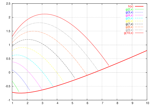
Let

	$\displaystyle g_{n}(x)$	$\displaystyle=$	$\displaystyle\log\left(\frac{n^{x}}{\sqrt{2\pi}x^{x+\frac{1}{2}}}e^{-\frac{1}{12x}}\right)$
		$\displaystyle=$	$\displaystyle x\log n-x\log x-\frac{1}{2}\log x-\frac{1}{12x}-\frac{1}{2}\log 2\pi$

(see figure 2). We first consider values of $x\geq 7$ . By hypothesis, $n/x\geq 4/3$ so $\log n-\log x\geq\log(4/3)$ , and therefore $g_{n}(x)\geq h(x)$ , where:

h(x)=x\log(4/3)-\frac{1}{2}\log x-\frac{1}{12x}-\frac{1}{2}\log 2\pi

(see Figure 2 also). Notice that $h(x)$ is independent of $n$ . The derivative of $h$ is

h^{\prime}(x)=\log(4/3)-\frac{1}{2x}+\frac{1}{12x^{2}}=\frac{12\log(4/3)x^{2}-6x+1}{12x^{2}}

The numerator vanishes at

x=\frac{1\pm 1\sqrt{1-4/3\log(4/3)}}{4\log(4/3)}

Numerically, $x\simeq 0.1867281114$ or $x\simeq 1.551301638$ . Therefore, the function $h(x)$ is increasing for $x\geq 2$ . Again, numerically $h(7)\simeq 0.1099761345$ and therefore, if $x\geq 7$ we always have:

e^{g_{n}(x)}\geq 1.1162>1

Now we consider $x\leq 6$ . Having $g_{n}>0$ , is equivalent to:

n>n_{0}(x)=xe^{\frac{1}{2x}\log x+\frac{1}{12x^{2}}+\frac{1}{2x}\log 2\pi}

At this point, we proved that $g_{n}(x)$ is positive, except possibly for pairs $(n,x)$ with $1\leq x\leq 6$ and $\frac{4}{3}x\leq n\leq n_{0}(x)$ . The values of $n_{0}$ are tabulated in Table 2. From Table 2 it is clear that the only exceptions are those listed in the hypothesis.

$x$ $\frac{4}{3}x$ $n_{0}(x)$ Possible $n$ ’s 1 1.333333333 2.724464424 2 2 2.666666666 3.844857634 3 3 4 4.939610298 4 4 5.333333333 6.016610872 5 5 6.666666666 7.081620345 6 6 8 8.137996302 8

Table 2: Possible values of

n

for

x

small

∎

{bibsection}

O^{*}(n^{5})

m